Munich Personal RePEc Archive
Distinguishing Between Spatial
Heterogeneity and Inefficiency: Spatial
Stochastic Frontier Analysis of European
Airports
Pavlyuk, Dmitry
Transport and Telecommunication Institute
2013
Online at
https://mpra.ub.uni-muenchen.de/65646/
Distinguishing Between Spatial Heterogeneity and Inefficiency: Spatial
Stochastic Frontier Analysis of European airports
Pavlyuk Dmitry
Candidate of Economic Science, Transport and Telecommunication Institute Lomonosova 1, Riga, LV-1019, Latvia
Phone: (+371)29958338. Email: Dmitry.Pavlyuk@tsi.lv
Keywords: airport efficiency, spatial stochastic frontier, maximum likelihood estimator
A problem of distinguishing between frontier heterogeneity and inefficiency is widely acknowledged in benchmarking. A special type of heterogeneity, based on the spatial structure, can significantly affect performance estimates in the airport industry. In this research we presented a general specification of the spatial stochastic frontier model which includes spatial lags, spatial autoregressive disturbances and spatial autoregressive inefficiencies. Maximum likelihood estimator has been derived for this model. Applying the suggested model specification to the European airports dataset, we discovered presence of significant spatial heterogeneity, which leads to biased estimates of efficiency, received using classical models.
Introduction
Airport benchmarking attracted significant scientific attention after industry liberalisation in the nineties [1], [2]. There are more than a hundred research papers, published during last two decades, and devoted to airports efficiency estimation. The most significant reports are the Global Airport Performance Benchmarking Reports produced by Air Transport Research Society[3], the Airport Performance Indicators and Review of Airport Charges reports by Jacobs Consulting, the Airport Service Quality programme by Airports Council International. Some local authorities which control the airport sector also provide their own benchmarking reports, e.g. Civil Aviation Authority (UK) [4], and others. Many related researches are also executed within the bounds of the German Airport Performance research project, a joint study between three German universities.
Despite intensified research of efficiency in the airport industry and obvious locational issues, spatial effects are rarely included into consideration. Spatial interactions between European airports and spatial heterogeneity of the industry structure are widely acknowledged [2] and should be included into airport benchmarking techniques ([5–7]).
Spatial relationship is usually presented in a form of spatial competition. Theory of spatial competition is well developed, but rarely applied to airports. Taking spatial interactions between airports into models is critically important for estimation of airports efficiency levels. A wide range of instruments like overlapping catchment areas, a network connectivity index and other were suggested, but the spatial econometric models can be highlighted as the most theoretically supported methodology.
Spatial heterogeneity is also a very important drawback in airport efficiency research. Region-specific settings can significantly affect airports activity, but their inclusion into a model is not straightforward. There are some sources of regional heterogeneity of airport activity:
-Climate. Airport activity can be significantly affected by a climate. For example, snow-belt airports have to spend additional efforts on runway service, which reduce their production in relation with airports located in a region with softer weather conditions. Mapping this difference out the model will lead to underestimated values of snow-belt airports’ efficiency.
-Economics. Economic situation in European countries is very heterogeneous. Significantly different income per capita and price levels define different demand to air transport.
-Region attractiveness. Regions also are not equal in relation to their demand for air transport. Business activities, required air flights, tourism attractiveness significantly vary across Europe. A standard approach to include these factors into the model is based on a set of region-specific dummy variables, and looks weak in case of a complex spatial structure. Spatial effects are usually not limited with country borders, so using of an administrative division in this case is not well-grounded. Nevertheless, spatial structure should be included into efficiency estimation to prevent a bias in efficiency estimates.
resources to produced outputs. This approach considers all deviations from the frontier as unit inefficiency and doesn’t take possible heterogeneity into account.
There are a number of different methods proposed to distinguish heterogeneity and inefficiency within the stochastic frontier models. The most frequently used approach is based on inclusion of variables, describing heterogeneity into the model (observed heterogeneity). For airports it can be geographical regions, ownership ([9], [10]), government regulation ([11]), and others. Another possible way to distinguish heterogeneity and performance relies on the time factor and assume that heterogeneity is more stable over time than inefficiency [12].
Despite a significant number of empirical applications, given methods have a number of shortcomings, generally related with their insufficient flexibility and requirements for initial assumptions. Spatial proximity is rarely used in such models, which generally leads to lose of information in case the spatial structure plays a role. Development of spatial econometrics [13] allows including spatial heterogeneity and spatial relationships into parametric models in a undisguised and flexible way. However spatial specification of the stochastic frontier model is insufficiently researched. In this research we consider a general form of the spatial stochastic frontier model with all types of spatial components – spatial lags, spatial autoregressive disturbances and spatial autoregressive inefficiencies.
A set of popular econometric techniques (maximum likelihood, two-step least squares, general method of moments) can be adapted estimation of this model. We develop a maximum likelihood estimator for different forms of the stochastic frontier model. Applying the developed estimator to a data set of European airports, we analysed an influence of spatial components on estimated airport efficiency.
Specifications of a spatial stochastic frontier model
A classical stochastic frontier model is usually presented in a matrix form as [8]:
,
0
,
,
≥
−
=
+
=
u
u
v
X
y
ε
ε
β
(1)
where
y is an (n x 1) vector of a dependent variable, output (n is a size of the sample);
X is an (n x k+1) matrix of explanatory variables, inputs (k is a number of explanatory variables); β is a (1 x k+1) vector of unknown coefficients (model parameters);
ε is an (n x 1) vector of composite error terms;
v is an (n x 1) vector of independent identically distributed (i.i.d.) error terms;
u is an (n x 1) vector of inefficiency terms with non-negative values.
The classical stochastic frontier model doesn’t include any spatial dependencies and assumes that all objects in a sample are independent. This assumption is too restrictive in some practical cases. Spatial effects can be presented almost in all components of the classical model:
-spatial influence of neighbours’ output values on a given unit’s output (spatial lags); -spatial influence of neighbours’ input values on a given unit’s output;
-spatial relationship between neighbour unit’s error terms (spatial heterogeneity); -spatial correlation between efficiency of neighbour units.
We define a general spatial stochastic frontier model, including all these effects into the classical stochastic frontier model specification:
,
0
,
~
,
~
,
,
4 3
2 1
≥
+
=
+
=
−
=
+
+
+
=
u
u
u
W
u
v
v
W
v
u
v
X
W
X
y
W
y
η
ξ
ε
ε
γ
β
ρ
(2)
W1y is a spatial lag vector of output values (with a coefficient ρ);
W2X is a spatial inputs-output lag vector (with a coefficient γ);
W3v are spatial errors (with a coefficient ξ);
W4u are spatial inefficiency lags (with a coefficient η).
Matrices W1, W2, W3, and W4 represent levels of spatial dependency between units (spatial weights) and can be different for every spatial component. All spatial weights matrices have zero values on the main diagonal (to prevent self-dependency). Construction of these matrices is usually research-specific and can be based on geographical distances, travel times, etc.
Estimation of the general spatial stochastic frontier model’s parameters is a complicated task, which is related with identification problems, computation performance issues and requires a significant volume of data. In this research we consider two special cases of the general spatial stochastic frontier model.
Let apply following constraints on the general spatial stochastic frontier model:
,
0
=
γ
(3), 0 =
ξ
(4).
0
=
η
(5)Under these constraints the model includes only spatial lags for unit’s outputs, all other spatial effects are excluded:
.
0
,
~
,
~
,
,
1
≥
=
=
−
=
+
+
=
u
u
u
v
v
u
v
X
y
W
y
ε
ε
β
ρ
(6)
Following LeSage [14] notation for naming of spatial models, this model is a mixed first-order spatial autoregressive-regressive stochastic frontier model. We will refer this model as a spatial autoregressive stochastic frontier (SARSF) model.
Another model we consider in this research includes spatial relationship of a symmetric error term v as well as spatial lags. Suppressing the constraint (4), we obtain the following model specification:
.
0
,
~
,
~
,
,
2 1
≥
=
+
=
−
=
+
+
=
u
u
u
v
v
W
v
u
v
X
y
W
y
ξ
ε
ε
β
ρ
(7)
We will refer this model as a mixed first-order spatial autoregressive-regressive stochastic frontier model with spatial autoregressive disturbances (SARARSF).
Maximum likelihood estimator for spatial stochastic frontier models
A wide range of statistical methods is used for estimation of spatial model parameters. The most popular are maximum likelihood estimator [13], [14], two-step least squares[15], and generalised method of moments[16], [17]. In this research we derive maximum likelihood estimators for SARSF and SARARSF models1.
The maximum likelihood estimator requires an assumption about distributions of error and inefficiency components. The distribution of the symmetric error term v is usually set to normal, and the distribution of the non-negative inefficiency term u is selected from half-normal[19], truncated normal [20], or gamma[21]. We consider the simplest normal-half-normal type of the composite error term ε:
).
,
0
(
~
~
),
,
0
(
~
~
2 ~ 2 ~
I
N
u
u
I
N
v
v
u v
σ
σ
+=
=
(8)
1
The probability density function for this case is well known:
( )
2 , − Φ =
σ
ελ
σ
ε
ϕ
σ
ε
f (9) where,
,
~ ~ 2 ~ 2 ~ v u v uσ
σ
λ
σ
σ
σ
=
+
=
φ and Φ are standard normal probability density and cumulative distribution functions accordingly.
Maximum likelihood estimator for the SARSF model
Derivation of the maximum likelihood estimator formula for the SARSF model (6) is quite straightforward. According to the model specification, the composite error terms vector can be expressed as:
(
ρ
)
β
ε
β
ρ
ε
ε
β
ρ
X
y
W
I
X
y
W
y
X
y
W
y
−
−
=
⇔
−
−
=
⇔
+
+
=
1 1 1Using the multivariate change of variables formula and the Jacobian matrix, we can produce the probability density function for y:
( ) ( )
det
(
1)
2
det
I
W
y
f
y
f
ρ
σ
ελ
σ
ε
ϕ
σ
ε
ε
−
−
Φ
=
∂
∂
=
(10)Now the log-likelihood function can be easily obtained:
(
)
( )
(
(
1)
)
1 2
1
ln
ln
det
2
ln
,
,
,
,
,
y
X
W
C
n
I
W
LogL
n i Tρ
σ
ελ
σ
ε
ε
σ
σ
β
ρ
+
−
−
Φ
+
−
−
=
∑
= (11)Maximum likelihood estimator for the SARARSF model
We follow the procedure, described in Kumbhakar and Lovell [8] to produce the probability density function and likelihood function for the SARARSF model (7).
Initial model specification includes the distribution of the error term in an implicit form:
).
,
0
(
~
~
,
~
2 ~ 2I
N
v
v
v
W
v
vσ
ξ
+
=
Straightforward transformations give us:
(
−
)
⇔
=
⇔
=
−
−v
W
I
v
v
v
W
v
~
~
1 2 2ξ
ξ
(
)
(
)
(
)
12 1 2 2 ~ 2 ~
~
where
),
,
0
(
~
N
Σ
Σ
=
Σ
=
I
−
W
−I
−
W
−v
σ
vσ
vξ
Tξ
(12)So the error term has a multivariate normal distribution with a covariance matrix Σ and its respective probability density function is given as:
( )
(
( )
)
Σ
−
⋅
Σ
⋅
=
− −v
v
v
f
T n 1 2 12
1
exp
det
2
1
π
(13)The half-normal probability density function is given as:
( )
<
≥
−
⋅
=
0
,
0
0
,
2
exp
2
2
2 ~ ~u
u
u
u
u
f
u T nu
π
σ
σ
(14)Assuming u and v components are independent, the joint normal-half-normal probability density function is a product of functions (13) and (14):
( ) ( ) ( )
(
( )
)
( )
(
)
Σ
+
−
Σ
=
=
−
⋅
⋅
Σ
−
⋅
Σ
⋅
=
⋅
=
− − − −v
v
u
u
u
u
v
v
v
f
u
f
v
u
f
T u T n u u T n u T n 1 2 ~ 2 1 ~ 2 ~ ~ 1 2 12
1
exp
det
1
2
exp
2
2
2
1
exp
det
2
1
,
σ
πσ
σ
π
σ
π
Since ε= v – u:
( )
(
( )
)
(
)
(
)
( )
(
)
(
(
)
)
Σ
+
Σ
+
Σ
+
Σ
+
−
Σ
=
=
+
Σ
+
+
−
Σ
=
− − − − − − − −ε
ε
ε
ε
σ
πσ
ε
ε
σ
πσ
ε
1 1 1 1 2 ~ 2 1 ~ 1 2 ~ 2 1 ~2
1
exp
det
1
2
1
exp
det
1
,
T T T u T n u T u T n uu
u
u
I
u
u
u
u
u
u
f
Straightforward transformations give a simplified form of the joint probability density function:
( )
(
( )
)
(
)
(
)
(
)
,
2
1
exp
2
1
exp
det
1
,
2 1 11 ~
Θ
−
−
Ω
−
−
Σ
=
−µε
−µε
ε
−ε
πσ
ε
T Tn u
u
u
u
f
(15) where.
,
,
1 1 2 ~ 2 ~ − −ΩΣ
−
=
ΣΘ
=
Ω
Σ
+
=
Θ
µ
σ
σ
u uI
The marginal density of ε is obtained by integrating u out of f(u, ε):
( )
( )
(
( )
)
(
)
(
)
(
)
( )
(
)
(
( )
)
(
( )
)
(
)
(
)
(
)
, 2 2 1 exp 2 1 2 1 exp det 2 1 det det 2 2 1 exp 2 1 exp det 1 , 2 1 2 1 1 0 1 2 1 2 1 2 1 ~ 0 1 1 2 1 0 Θ Ω Φ = = Θ − − Ω − − Ω Ω Σ = = Θ − − Ω − − Σ = = − − − ∞ − − − ∞ − − − ∞∫
∫
∫
ε ϕ µε ε ε π µε µε π σ ε ε µε µε πσ ε ε n T n T n n u T T n u du u u du u u du u f fwhere φ(x, mean, covariance) and Φ(x, mean, covariance) are multivariate probability density and cumulative distribution functions with a mean vector mean and a covariance matrix covariance.
So finally the probability density function of the composite error term ε is obtained:
( )
ε =2n(
Φ(
0,µε,Ω)
) (
ϕε,0,Θ)
f (16)
Using the density function (16) and following the same logic as in (10), we obtained the respective log-likelihood function for the SARARSF model:
(
y
|
,
~,
~,
)
C
ln
(
(
,
,
)
)
ln
(
(
,
,
)
)
ln
(
det
(
I
W
1)
)
,
LogL
β
σ
vσ
uρ
=
+
Φ
0µε
Ω
+
ϕ
ε
0Θ
+
−
ρ
(17) where.
~
,
~
,
~
,
~
1 2 ~
1 2 ~ 2 ~
2 ~ 2 ~ 2 ~
− −
−
Σ
Ω
−
=
Θ
Σ
=
Ω
Σ
+
=
Θ
Σ
=
Σ
v v u
v u v
I
σ
µ
σ
σ
σ
σ
σ
Maximisation of the log-likelihood function with respect to its parameters is a separate computational problem.
Application to airports
We applied both SARSF and SARARSF specifications of the spatial stochastic frontier model to a data set of European airports.
There are many different approaches to understanding of airport business, a set of used resources and an output of airport activity [23]. In this research we used a number of transferred passengers of a main result of airport activity and infrastructure units (gateways, check-ins) as airport resources. The production function used in this research is estimated in the form (SARARSF model):
(
)
(
)
(
)
(
)
)
,
0
(
~
)
,
0
(
~
~
,
~
,
ln
ln
ln
ln
2 ~
2 ~
3 1
0
I
N
u
I
N
v
v
Wv
v
u
v
CheckIns
Runways
Passengers
W
Passengers
u
v
σ
σ
ξ
β
β
ρ
β
+
+
=
−
+
+
+
+
=
(18)
where
Passengers is a total number of passengers carried by an airport (both departure and arrival);
Runways and CheckIns are numbers of airport’s runways and check-ins respectively. Other airport infrastructure characteristics are excluded due to a multicolleniarity problem.
A matrix of spatial weights W was constructed on the base of Euclidean distances. Realising all shortcomings of this approach, we think that general influence of spatial effects will be estimated correctly.
Data
The study data set includes characteristics of 122 European airports in 2009. The characteristics include:
- A number of passengers carried (direct transit passengers are excluded). This indicator is used as the main output of airport’s activity.
- Airport infrastructure – a number of check-in facilities, gates, runways, and parking spaces are used as input resources of airports’ activity.
The full dataset is collected from the Eurostat database [24]. Descriptive statistics of the collected dataset is presented in the Table 1.
Table 1. Data descriptive statistics
Total number of passengers carried,
thousands
Number of runways Number of check-ins
Min 108.0 1 3
Median 4479.8 2 43.5
Max 60495.8 6 481
Estimation results
Three different model specifications were tested for the data set: - classical stochastic frontier (SF estimates);
- spatial autoregressive stochastic frontier (SARSF estimates);
- spatial autoregressive stochastic frontier with spatial autoregressive disturbances (SARARSF estimates).
The results are presented in the Table 3.
Table 2. Estimation results of different model specifications*
SF SARSF SARARSF
β0 12.498
(<2E-16)
12.50 (<2E-16)
12.120 (<2E-16)
β1 0.669
(7.3E-07)
0.668 (9.4E-07)
0.653 (5.7E-07)
β2 0.785
(<2E-16)
0.786 (<2E-16)
0.796 (<2E-16)
σv 0.549 0.444 0.494
σu 0.248 0.400 0.005
ρ - 0.0001
(9.4E-01)
0.0002 (9.0E-01)
ξ - - 0.132
(4.7E-08) * Values in brackets are significance
Standard SF estimates show significant inefficiency in data (inefficiency variance σu=0.248, which is
comparable with the error term variance σu). Moran’s I is a popular test statistics for spatial dependence [25]:
normal
d
i
i
e
e
We
e
MoranI
TT
.
.
.
~
=
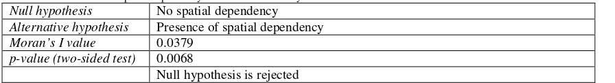
[image:8.595.76.524.527.588.2](19) Applying the Moran’s I test to estimated efficiency levels of the standard SF model, we strongly reject a hypothesis about absence of spatial relationships in data (see Table 3). Note that observed Moran’s I value is positive, which indicates positive spatial relationship.
Table 3. Moran’s test for spatial dependency in estimated efficiency values
Null hypothesis No spatial dependency
Alternative hypothesis Presence of spatial dependency
Moran’s I value 0.0379
p-value (two-sided test) 0.0068
Null hypothesis is rejected
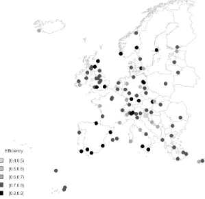
Spatial distribution of SF estimates of efficiency levels is presented on the Figure 1. We can note that efficiency levels are not distributed uniformly, having areas with higher (dark circles) and lower (light circles) values.
Figure 1. Spatial distribution of European airports efficiency
The SARSF model shows insignificant spatial lags and significant inefficiency. Taking spatial heterogeneity into account (SARARSF model) we produce alternative results. The SARARSF model demonstrates significant spatial heterogeneity in data (which is expected for the airport industry), and this spatial component supplants inefficiency – it becomes insignificant. This result is expected due to incompleteness of the production function components (only infrastructure metrics are included), but from our opinion the general findings are very important for further analysis. Generally, imperfection of the production frontier can produce incorrect conclusions about the inefficiency term, when including spatial components into the model can partly improve the situation.
Estimates of input elasticises (coefficient β1 for a number of runways and coefficient β2 for a number of
check-ins) are quite stable for all models, which is reasonable in absence of significant spatial lags.
Conclusions
In this research we presented a general specification of the spatial stochastic frontier model which includes spatial lags, spatial autoregressive disturbances and spatial autoregressive inefficiencies. These spatial components describe present spatial relationships and spatial structure of study units and critically important for econometric models, specifically for efficiency estimation. Maximum likelihood estimator for the spatial autoregressive stochastic frontier with spatial autoregressive disturbances is derived.
an important evidence of necessity of spatial components in stochastic frontier models. Non-inclusion of spatial components into benchmarking models can lead to significant biases of frontier parameters and efficiency levels estimates.
Acknowledgement
The author is grateful to Jiaxian Lin, South China University of Technology, for providing materials and very useful comments on the maximum likelihood estimation of the spatial autoregressive stochastic frontier model.
References
1. Adler, N., Liebert, V. (2011). Competition and regulation (when lacking the former) outrank ownership form in generating airport efficiency, presented at the GAP workshop “Benchmarking of Airports,” Berlin, Germany, p. 27.
2. Pavlyuk, D. (2012). Airport Benchmarking and Spatial Competition: A Critical Review, Transport and Telecommunication, Vol. 13, No 2, pp. 123–137.
3. Oum, T.H., Yu, C., Choo, Y. (2011). ATRS Global Airport Performance Benchmarking Project, The Air Transport Research Society.
4. The Use of Benchmarking in the Airport Reviews (2000). Civil Aviation Authority, London, UK. 5. Barros, C.P., Managi, S., Yoshida, Y. (2008). Technical Efficiency, Regulation, and Heterogeneity in
Japanese Airports, School of Economics and Management, Lisbon, Portugal, Working Paper 43/2008/DE/UECE.
6. Barros, C.P. (2012). Performance, heterogeneity and managerial efficiency of African airports: the Nigerian Case.
7. Liebert, V. (2010). External heterogeneity in airport benchmarking and efficiency analysis, Jacobs University, Bremen, Germany.
8. Kumbhakar, S.C., Lovell, C.A.K. (2003). Stochastic frontier analysis. Cambridge: Cambridge Univ. Press, 344 p.
9. Adler, N., Liebert, V. (2011). Joint Impact of Competition, Ownership Form and Economic Regulation on Airport Performance, Jacobs University Bremen.
10. Barros, C.P., Marques, R.C. (2008). Performance of European Airports: Regulation, Ownership and Managerial Efficiency, School of Economics and Management, Lisbon, Portugal, Working Paper 25/2008/DE/UECE.
11. Malighetti, P., Martini, G., Paleari, S., Redondi, R. (2007). Efficiency of Italian airports management: the implications for regulation, Italy, Working Paper.
12. Greene, W. (2003). Distinguishing Between Heterogeneity and Inefficiency: Stochastic Frontier Analysis of the World Health Organization’s Panel Data on National Health Care Systems.
13. Anselin, L. (1988). Spatial econometrics: methods and models. Dordrecht: Kluwer Academic Publishing, 304 p.
14. LeSage, J.P. (1999). Spatial econometrics. Regional Research Institute, West Virginia University, 296 p. 15. Kelejian, H.H., Prucha, I.R. (1998). A generalized spatial two-stage least squares procedure for
estimating a spatial autoregressive model with autoregressive disturbances, The Journal of Real Estate Finance and Economics, Vol. 17, No 1, pp. 99–121.
16. Druska, V., Horrace, W.C. (2004). Generalized moments estimation for spatial panel data: Indonesian rice farming, American Journal of Agricultural Economics, Vol. 86, No 1, pp. 185–198.
17. Lee, L. (2007). GMM and 2SLS estimation of mixed regressive, spatial autoregressive models, Journal of Econometrics, Vol. 137, No 2, pp. 489–514.
18. Pavlyuk, D. (2012). Maximum Likelihood Estimator for Spatial Stochastic Frontier Models, in
Proceedings of the 12th International Conference “Reliability and Statistics in Transportation and Communication” (RelStat’12), Riga, Latvia, pp. 11–19.
20. Stevenson, R. (1980). Likelihood Functions for Generalized Stochastic Frontier Functions, Journal of Econometrics, No 13, pp. 57–66.
21. Greene, W.H. (1990). A gamma-distributed stochastic frontier model, Journal of econometrics, Vol. 46, No 1–2, pp. 141–163.
22. Lin, J., Long, Z., Lin, K. (2010). Spatial Panel Stochastic Frontier Model and Technical Efficiency Estimation, Journal of Business Economics, Vol. 223, No 5, pp. 71–78.
23. Doganis, R. (1992). The airport business. London: Routledge, 240 p.
24. European Statistics Database (2012). Statistical Office of the European Communities (Eurostat). 25. Moran, P.A.P. (1950). Notes on Continuous Stochastic Phenomena, Biometrika, Vol. 37, No 1–2, pp.