Enrollment costs, university quality and higher education choices in Italy

(1)

Munich Personal RePEc Archive

Enrollment costs, university quality and

higher education choices in Italy

Pigini, Claudia and Staffolani, Stefano

University of Perugia, Università Politecnica delle Marche

3 October 2013

(2)

Enrollment costs, university quality and higher

education choices in Italy

Claudia Pigini Stefano Staffolani ∗

Abstract

In this paper, we analyze the higher education choices of Italian secondary school leavers by addressing the roles of university quality, costs and geographical distance to the institu-tion as well as the relainstitu-tionship between students’ choices and their personal and household’s attributes, such as individual secondary school background and the socio-economic con-dition of the family of origin. Grounding such decision process on the framework of the Random Utility Model (RUM), we provide empirical evidence on the determinants of stu-dents’ choices by estimating a nested logit model on the ISTAT survey of secondary school graduates. Results show that the effects of increasing costs of enrollments and university standards are strongly differentiated across sub-groups of individuals. In particular, the choice probability of weaker students, in the sense of secondary school background and household’s socio–economic condition, is more sensitive to changes in university costs and quality.

Keywords: Enrollment cost, university quality, geographical distance, university choice, Ran-dom Utility Maximization model.

JEL classification: C25, I21, I23, J24

1 Introduction

The last decade has seen a growing interest in understanding the behavior of high school grad-uates when facing the decision of whether to participate in higher education and, if so, where to enroll. In the Italian case, critical policy issues are the low rate of participation in higher education1 and low mobility of secondary school leavers who, therefore, may not enroll into the institution better matching their ability and preferences. Recently, the Italian government is-sued a ministerial decree to found initiatives aimed to subsidize students’ geographical mobility

2_.

The Italian university system is characterized by free-admission: the only requirement to enroll is “Maturit`a”, the secondary school diploma, that allows students to send an application

∗_{Claudia Pigini, Department of Economics, Finance and Statistics – University of Perugia (Italy). E-mail:}

pigini@stat.unipg.it. Stefano Staffolani (corresponding author), Department of Economics and Social Sciences

– Universit`a Politecnica delle Marche, P.le Martelli 8, 60121 Ancona (Italy) E-mail: s.staffolani@univpm.itTel:

+39-071-2207090, Fax: +39-071-2207102. 1

Only 20.2% of Italians between 25 and 34 graduates compared to the 37.1% of the OECD average (OECD, 2011)

2

(3)

to any Italian University in any subject3_{. Although it is required to pass admission tests to}

ac-cess degree courses in several countries (Anglo-Saxon, China, South-Eastern Asia and Southern American), free-admission is adopted in many European countries: the admission systems of Austria, Switzerland, Belgium, Sweden, Norway, Finland, Denmark, Portugal, Greece, France and Germany are very similar to the Italian one since they only require the secondary school diploma for enrollment4. Recently, the adequacy of the free-entry principle has prompted a very a lively debate in both Italy and Germany: starting in 2010, Italian universities were compelled to evaluate all enrolled students with a test, that is nevertheless not binding for admission; recently, in Germany, students cannot enroll into the most popular degree courses unless they have scored a minimum grade point average on their “Abitur”.

However, in a context as such as the Italian one, where the selection process is minimal, the choice of whether and where to go to university is almost entirely on the hands of the student once she/he has obtained a secondary school diploma. In this framework, university costs and quality play a central role in the higher education choices of secondary school leavers.

Students contribute to the financing of university studies in Italy by paying an enrollment fee that, on average, it is fixed at about 1000 Euros per year. Even though university cost is relatively low compared with the ones of other European and Anglo-Saxon countries, Italy has still one of the lowest rates of inter-generational mobility (Checchi, Fiorio, and Leonardi,2013) and the issue of raising the enrollment rate of poorer students has been recently re-addressed (see, for example,Ichino and Terlizzese(2013)). Furthermore, the financial situation of Italian government has lead to a drastic cut in the public financing of universities and to a growing demand for raising tuition fees by the university managements.

The low quality of the Italian higher education system is another major concern: in the 2013 National Higher Education Systems ranking of the Institute of Applied Economic and Social Re-search University of Melbourne, Italy is 29th out of the 50 countries analyzed5. The government recently intervened in the quality evaluation of Italian Universities by establishing a National Commission (ANVUR): its aim is to measure the quality of university activities by quantita-tive indicator that consider the efficiency of teaching, the quality of the scientific research, the capability of collecting private financing, and the adequacy of public communication.

In the light of this debate, this paper examines the enrollment decision and the choice of which university to attend of Italian secondary school graduates. Recently, few contributions have analyzed university choices in Italy mostly addressing the geographical accessibility of the higher education system and the financial constraints affecting students’ participation decisions. The empirical evidence, however, is limited to macro–geographical areas and it is not related to the private cost of enrollment nor to the university quality. Moreover, the available em-pirical studies do not consider how university choices may depend on the student’s personal characteristics combined with the single perspective institution attributes.

Our paper adds to the existing literature by developing an empirical framework grounded on the Random Utility Maximization (RUM) model that describes the student’s choices of enrollment and attendance in terms of both universities attributes and individual characteristics. We address the roles of university quality, costs and geographical distance to the institution as well as the relationship between students’ choices and their personal and household’s attributes, such as individual secondary school background and the socio-economic condition of the family of origin.

3

The exceptions are the faculties of medicine and architecture. A number of applicants, decided a–priori, is selected after an entry test.

4

A complete list of countries with free post-secondary education is available athttp://en.wikipedia.org/

wiki/Free_education

5

(4)

We provide empirical evidence by estimating a nested logit model for students’ university participation and choice. The use of probabilistic choice models for higher education decisions was first advocated byManski and Wise(1983) and followed in recent analyses byLong(2004),

Drewes and Michael (2006) and Gibbons and Vignoles (2012) who estimate conditional logit

models. While appealing for its simplicity and speed of implementation, a limitation of the conditional logit model is assumption of Independence of Irrelevant Alternatives (IIA), that is the choice between any pair of universities is independent of the attributes of any other available option. The assumptions underlying the nested logit model allow us to dispose of the IIA within groups of comparable alternatives6.

We use the Italian Institute of Statistics (ISTAT) survey of secondary school graduates in 2004 interviewed in 2007 linked with data on university attributes from the Italian Ministry of Education, University and Research (MIUR). Moreover, we use as university quality indicator the 2003 popular university score of Censis-Repubblica. We add the information on the socio– economic condition of Italian provinces in 2003 using the indicators published by the magazine Il Sole 24 Ore. Such level of detail makes this a unique dataset that has never been used to investigate the factors influencing the decision to participate in higher education and institution choice of Italian secondary school leavers.

Our main results are presented in form of elasticities of the choice probability to geographical distance, university standard and tuition fees computed for the whole population of students and for sub-groups of secondary school leavers divided according to different personal and family attributes. The elasticity to distance ranges from −3.0%, for students with a diploma from a vocational school and a secondary school low final grade, to −0.1%, for students coming from “Liceo” and whose mother has a university degree. The elasticity to tuition fees ranges from

−3.2%, for student with a vocational diploma and the lowest secondary school grades, to 0 for students coming from Liceo and with the highest secondary school grade. For the same groups of students, the elasticity to university standard is 4.2% and 0, respectively. “Weaker” students, in the sense of a weaker secondary school background and a family income and level of education, are more sensitive to changes in enrollment costs and quality of the academic institutions. An increase in enrollment costs, measured by both geographical distance and tuition fees, has an effect that is strongly differentiated between sub-groups of the population.

The remainder of the paper is organized as follows: Section 2 reviews the recent Italian and international contributions on students higher education choices; Section 3 illustrates the theoretical framework for the participation decision and institution choice on which we base our empirical evidence; Section 4 describes the dataset and the variables of interest, and Section

5.1presents the estimation results. Finally, Section 6concludes.

2 Literature review

There are only a few studies that analyzed the university choices of secondary school leavers in Italy. In these works, considerable attention has been given to the geographical accessibility of the higher education system and to the possible financial constraints affecting the students’ choices. Most recently, Cesi and Paolini (2011) developed a theoretical model predicting that geographical distance is a strong deterrent to university participation and choice. Ordine and Lupi (2009) also show that mobility is constrained by family income: Italian students tend to choose a university located in their own region despite the Italian university system offers different quality standards which may allow a more efficient ability sorting of students across

6

(5)

institutions. In addition, the results form the gravity model inAgasisti and Dal Bianco(2007) suggest that when a student moves, chooses a university located in an area with good socio-economic conditions rather than choosing on the basis of that university’s attributes.

While Italian contributions have only explored the choices of whether and where to attend university related to geographical mobility, more extensive analyses have been carried out for other countries: a wider range of factors, such as tuition fees, university quality and individual characteristics, has been considered. Evidence suggests that the high school background is a prevailing factor in deciding whether to attend university. Long(2004) examines both the deci-sion of enrolling and into which college for the US from 1972 to 1992. Tuition and geographical distance negatively affect the decision of which college to attend while college quality has an important role in attracting students who decide to enroll. Alm and Winters (2009) confirm the key role of distance in the choice of where to study also for Georgian intrastate migration. In the case of Canada, Frenette (2004) and (2006) show that the likelihood of attending local colleges increases when the the student lives, on average, fare from her possible choices and the participation rate is low for those who live too far to even commute. In addition, Drewes and

Michael (2006) suggest a somewhat convex relationship between tuition fees and probability of

choosing a certain university: the negative effect of price attenuates when for high amounts of tuition fees charged as they may be associated by students with the supply of better services. Moreover, their empirical evidence suggests that enrolled students are efficiently sorted across institutions: universities that require low standards for admission attract less talented students, while students with high ability are more attracted to high quality institutions. The cases of Netherlands and Flanders are examined by S´a, Florax, and Rietveld (2004) and Verboven

and Kelchtermans(2010) respectively. S´a, Florax, and Rietveld(2004) stress that geographical

proximity has a key role in the enrollment probability along with the students ability and school background (a similar result can be found in Spiess and Wrohlich (2010) for Germany and in

Denzler and Wolter (2011) for Switzerland). The choice of which subject to study is included

in the analysis of Verboven and Kelchtermans (2010): distance and travel costs are a strong deterrent for the choice of where and what to study, while they do not affect the participation decision. Gibbons and Vignoles (2012) found a similar results for the case of UK where geo-graphical distance negatively affects the choice of the institution and this effect is stronger for students coming from lower socio-economic groups. As in Verboven and Kelchtermans(2010), also in the UK there is only a weak link between geographical distance and the participation decision.

3 An empirical model for the enrollment decision and university

choices

In this section, we infer on the factors affecting enrollment decisions of secondary schools leavers, by considering heterogeneity both in the demand (individuals) and the supply (universities) sides of higher education. The aim is to provide theoretical ground to the use of the RUM and to evaluate the role played by financial constraints in the choice of which university to attend. For the demand side we assume that:

Assumption 1 Each individual i lives in a specific geographic area zi (district hereafter), is naturally endowed with a given talent ti, lives in a family willing to finance the student’s uni-versity studies with an amount mi, and has completed secondary school in a specific field of study.

(6)

Assumption 2 Each universityj is located in a specific districtzj, sets tuition fees at the level

fj, and is characterized by the standard sj.

By university standard, we indicate the quality of the institution that we assume influences both level of commitment required to the student to graduate, in terms of studying, and the expected labor income.

Assumption 3 The probability of graduation pij of individual i in university j depends posi-tively on the student’s talent ti, negatively on the university standard sj, and positively on the proximity 0≤πij ≤1, by which we indicate the degree of similarity between the fields of study offered by university j and the student’s secondary school field of study. Labor income depends positively on the university’s standard: it is higher for university graduates than for individuals with a secondary school diploma. Dropping-out gives the same income as non-enrollment.

We define U as the per–period utility that depends on consumption that, once the labor market is entered, is equal to the wage rate; we also define V as the expected inter–temporal utility so that V = U_r, where r is the discount rate. Therefore, V_ijG = w(sj)

r is the expected utility of the graduate student iin university j depending on w(sj) that is the expected wage rate of graduates of universityj;VN = ω

r is the expected utility of both non enrolled secondary school leavers and dropouts, where ω < w(sj) forj = 1, . . . , J is the wage rate of the unskilled. For a secondary school graduate living in district zi who may choose to enroll in one of the

J universities, the expected utility of enrollment V_ijE can be written as:

V_ijE =U(cij) +pij

V_ijG

1 +r + (1−pij)

VN

1 +r forj = 1, . . . , J (1)

where the first term on the right hand side7 is the per-period utility of studenti that depends on consumptioncij. The expected long–life utility of graduates the expected long–life utility of non–graduates are weighted by the probability of graduation in universityj (pij).

Consumption cij in (1) is also university-specific and is assumed to depend negatively on the geographical distance dij between the student’s district of residence zi and the district where university j is located, zj, because of transportation costs. Consumption also depends negatively on the cost of living in zj, hj, and on the tuition fee set by university j, fj (see Assumptions1and2). It depends positively on the amount the family of studentiis willing to pay for university study, mi (see Assumption1). Therefore we can write:

cij =mi−fj−φ(dij)−hj (2)

where the function φ() is non-linear since transportation costs are not proportional with re-spect to the distance between the student’s residence and the university location: the cost of commuting is increasing up to the point at which moving is more convenient than commuting; when a student moves, leaving out living costs, the transportation cost increases less than pro-portionally with respect to the geographical distance unless very large distances are considered. It is, therefore, reasonable to conjecture thatφ() as a cubic function.

The student optimal choice is the one that satisfies the following:

Remark 1 If Vij < VN, for j = 1, . . . , J, student i does not enroll. If Vij > VN, for at least one j, student ienrolls. Student ichooses university kif Vik> Vij∀j6=k.

7

(7)

Let us now examine Remark (1) in the special case where consumption during the studies does not depend on the chosen university, so that cij =ci: we are assuming that the student’s family is willing to finance any choice of the student or, alternatively, that the government finances completely the student’s university studies. In this special case, the enrollment decision depends only on the expected long–life utilities of graduation and dropping out weighted by the graduation probability (see equation (1)) and it is not affected by the consumption during the studies. By assuming thatsis continuous and that each university offers all the fields of study (πij = 1∀i, j), we can rewrite equation (1) as:

V_iE =U(ci) + 1

r(1 +r)[p(ti, s)(w(s)−ω) +ω] (3)

where p(ti, s) = pi for clarity in the following derivations 8. In order to find the university standard that coincides with the student’s optimal choice, we derive (3) with respect to s

obtaining the following FOC:

dp(ti, s)

ds (w(s)−ω) +p(ti, s) dw(s)

ds = 0

where the first addend is negative and the second is positive as per Assumption 3. Solving in sthe FOC, we obtain s∗_{, the standard that maximizes the expected utility after the study} period9. This standard defines the optimal university, j∗. If V_ijE∗ > VN, student i prefers to

enroll.

This result implies that for each secondary school leaver there exists a standard s∗ _that maximizes her expected utility in this special case.

Remark 2 If studentienrolls and if universityk, as defined in Remark1, is different from the one offering the optimal standard s∗, or if the non–enrollment decision is made but V_ijE∗> VN,

the choice of student i is sub–optimal because of financial constraints.

Therefore, if moving decisions were completely financed (by the family or the government) and if all standards and fields of study were offered, the standards∗ would always be chosen by all enrolled individuals. In this case, the individual utility would depend positively on talent alone. However, the majority of secondary school leavers are likely to be financially constrained. In that case, tuition fees and the cost of living in each district become crucial for the choice of university. Furthermore, the standard sis not continuous and universities usually do not offer all the fields of study, so πij can be lower than 1. Sub–optimal choices can therefore be made.

Let us now return to the more general case where consumption during studies does depend on the chosen university and the student’s decisions are affected by financial constraints. From Remark 1, the probability that studentienrolls in university k,Pik, is therefore:

Pik = ProbVikE(ti, sk, πik, cik)> VijE(ti, sj, πij, cij)

V_ikE(ti, sk, πik, cik> VN)∀j6=k. (4)

Let us now relax the assumption on the conditioning set in equation (4), that is we assume that studenti chooses from a set ofJ+ 1 alternatives that includes theJ universities and the non–enrollment option obtaining

Pik= Prob [Vik(ti, sk, πik, cik)> Vij(ti, sj, πij, cij)] ∀j 6=k in j = 1, . . . , J + 1.

8

We dropped the j index as the utility has to be maximized with respect tosthat is assumed to be continuous.

9

We obtain a maximum if d2_p

ds2(w(s)−ω)+2dpds dw ds+p(s)

d2_w

ds2 <0, that we assume to be respected. For instance,

(8)

This is aJ+ 1–choice multinomial model that can be designed as an Additive Random Utility Model by specifying V as:

Vij =d′ijβ+x′jγ+wijδ+υij for i= 1, . . . , N, j = 1, . . . , J + 1. (5)

In this specification, dij is a set of covariates that approximates the function φ() of the geo-graphical distance between the residence of student i and the location of university j in (2). The vector xj contains the supply side attributes, that are the university standard, fees, the consumption during studies (here depending only on the cost of living in zj, hj) and other control variables qj, so that xj = [sj, fj, hj,qj]. Finally, the vector wij is a set of covariates that includes interactions between the supply side variables of interest (geographical distance, standard and fees) and covariates that approximate individual characteristics such as the stu-dent’s household socio–economic condition mi and the student’s talent ti related to her high school background10.

The assumption on the distribution of the error termυij determines the type of probabilistic choice model to be estimated. Despite its appealing ease of implementation, the conditional logit model adopted in recent contributions (see section 1) is unsuitable for our problem as it requires that the choice between pairs of alternatives is independent of the attributes of the other options. To completely remove the Independence of Irrelevant Alternatives assumption, a random parameter logit should be estimated. However, as it will be shown in the next section, the extremely high number of student–alternative combinations in our dataset makes the estimation of a mixed logit model unfeasible. Instead, to overcome the IIA limitation, we estimate a nested logit model and allow group of alternatives to be dependent.

We estimate a two–level model of simultaneous choices where: 1) at the first level the student chooses between 5 options, non–enrollment and four fields of study (scientific, medical, social sciences, and humanities); 2) at the bottom level the student chooses among all possible combinations of Italian universities and field of study, where available11. This structure allows the bottom level alternatives to be correlated within each field of study, while the five higher level sets are independent of one another. This assumption seems plausible as the entire supply of Italian university faculties are aggregated in macro groups that are closely related to the secondary school fields of study as also to the choice of not to enroll. We, therefore, assume that theυij are distributed as generalized extreme values (GEV) and the parameters in (5) can be estimated by Full Information Maximum Likelihood12.

The main interest of our analysis is to investigate how changes in the supply–side attributes affect the student’s probability of choosing a given university in relationship with her individual and household characteristics. To this aim, it is useful to compute direct marginal effects and elasticities.

In the nested logit model, the marginal effect of a change in a generic university attributeyj on the probability that studentichooses one of the bottom level alternativesjcan be computed as

10

The nature of the multinomial model does not allow identification of parameters associated with alternative–

invariant regressors. A possible strategy would be to interact alternative–invariant characteristics with

alternative–specific intercepts. However, as we will see later in this paper, the choice set is far to large for this strategy to be implemented. We prefer using interactions with continuous university covariates for both computational parsimony and focus of the analysis.

11

It simply means that there are universities (as in Rome or Milan) that host all four fields of study, while there are some that can even offer only one of them.

12

For brevity, we do not treat in depth the technical details of the nested logit model estimation. Instead, we

(9)

[image:9.595.143.455.105.217.2]

Table 1: Variables’ sources used in the estimation of the nested logit model

ISTAT MIUR CENSIS SOLE 24 ORE

Father’s occupation Fees Standard Rent

Mother’s education Private Population

Final grade Quality of life

Secondary school type Closed N. of faculties Distance

Proximity Unemployment*

* ISTAT labor force survey

ψij,yj = ∂Pbij

∂yj =Pbij

1−Pbij

ϕ(yj,τ) (6)

where φ(yj,τj) = ∂V_∂yij_j and τ is a vector of parameters that includes elements of (β′,δ′)′ or (γ′,δ′)′. Given the high number of students and alternatives in our dataset, we rely on the computation of some average quantities to compute marginal effects and elasticities. So, for instance, we compute

εi,y¯= ¯ψi,yj

¯

y

e

Pi

(7)

where ¯ψj,yj =

1 J+1

PJ+1

j=1 ψij,yj, Pei =

P

j6=nePˆij and ¯y = J+11

PJ+1

j=1 yj. where we write ne as non-enrollment for clarity.

4 Data and variables

In this section, we describe in detail the variables used for the estimation of the RUM. Since our analysis contains variables at both the individual and university level, we matched information from various sources; moreover, we added some information on the socio-economic characteris-tics of the provinces the universities are located in. The sources used to build our variables are summarized in Table1.

(10)

In analyzing the students’ university choices, the individual attributes we focus on are the socio-economic condition of the student’s household and the student’s secondary school back-ground. As proxies of the socio-economic status of the student’s family of origin, we used the categorical variables “Father’s occupation” and “Mother’s education”13_{. The first variable}

in-dicates if the father’s occupation is blue collar or unemployed (BC/unem.), white collar (WC), self-employed (Self-em), or chief executive officer (CEO). The second variable indicates the mother’s level of education as follows: primary school or no education, lower secondary school, upper secondary school, degree or higher. As an indicator of the student’s secondary school record, we used the “Final grade” (which ranges from 60 to 100) that the student obtains with her/his secondary school diploma. This measure has been normalized by the students’ sec-ondary school of provenance and divided in four classes using quartiles. Finally, we included the “Secondary school type” that indicates if the student attended a vocational school, a tech-nical school, a Liceo or other institutes that are mostly dedicated to prepare students for the teaching carrier (Pedagogical). Typically, more talented students enroll into Liceo (that offers two possible curricula: humanities or sciences) after completing the lower secondary school.

The first two columns of Table2show the sample composition for these individual variables. It emerges that the participation in higher education is strongly differentiated according to all the characteristics presented in the table. The household socio–economic condition is a strong source of differentiation for the enrolling decision: the enrollment rates of students whose father is a white collar or a CEO are sensibly higher than those of other students and this percentage rises from 38% to 88% when comparing the lowest and highest levels of the mother’s education. Moreover, the 94% of students coming from Liceo decides to attend university while this percentage is much lower for students coming from vocational schools (30%). The secondary school final grade also plays a major role, by rising the probability of enrollment from 44 to 79% across its distribution.

The other key information contained in the ISTAT data is the student’s province of residence during the attendance of secondary school. Therefore, for each individual, we were able to compute the distance between the student’s province of residence and the province of each Italian university, measured in 100Km. The model specification also includes square and cube of distance. This variable takes value zero for universities located in the same province of the student’s residence during secondary school studies and for the non-enrollment option. The average distances between the students’ province of residence and the chosen university are displayed in the third column of Table 2 by individual characteristics: students coming from a household in a better socio-economic condition and more talented students seem to be more willing to move to a greater distance in order to attend the university studies.

For the purpose of the analysis, we linked the ISTAT dataset with other information on universities form multiple sources. As we want to investigate the effect of university quality on students’ choices, we used, as a proxy, the variable “Standard” which is the popular Italian university score of Censis-Repubblica (issued in 2003). This university score is currently used to infer on the quality of Italian Universities. It is built on five different classes of quantitative indicators: a)Productivity, that depends on the drop-out rate, on the average number of passed exams on the number of legal exams, and on other measures of the average actual length of the studies; b)Teaching, that considers the number of offered courses weighted by teachers, the ratio among students and teachers, the quantity and quality of infra-structures devoted to students, the survey-based students perceived opinion on courses and exams; c) Research, that mainly takes account of the public financing of research project; d)Teachers, that consider the average teachers’ age and the quality of their research; e) International cooperation , that analyses the

13

For a more detailed discussion on the role of the mother’s educational attainment in transmission of human

(11)

[image:11.595.100.496.213.631.2]

Table 2: Sample composition, enrollment rate, average distance, university standard, and tuition fees by individual characteristics.

Sample Enrollment

comp. (%) rate (%) Distance Standard Fees

Father’s occupation

BC/unem. 43.3 47.6 0.81 8.78 7.48

WC 17.3 67.6 0.86 8.83 7.97

Self–em 15.5 52.8 0.93 8.85 8.15

CEO 23.9 76.5 1.07 8.88 9.51

Mother’s education

Primary 12.3 38.2 0.76 8.75 7.21

Lower sec. 40.8 48.3 0.82 8.82 7.79

Upper sec. 38.6 70.1 0.92 8.85 8.52

Degree 8.4 87.9 1.27 8.85 9.57

Final grade

1st 25.0 44.3 0.86 8.83 8.03

2nd 25.0 50.6 0.83 8.84 8.24

3rd 25.0 61.7 0.93 8.83 8.26

4th 25.0 78.6 1.00 8.82 8.54

Secondary school type

Vocational 28.7 30.1 0.78 8.81 7.60

Technical 31.0 54.2 0.78 8.83 7.78

Liceo 21.3 94.4 1.17 8.84 9.08

Pedagogical 18.9 69.8 0.79 8.83 8.25

Total N. obs 25,277 58.8 0.92 8.83 8.30

(12)

number of Erasmus students on enrolled, teachers international mobility, their co-partnership to international research projects. This variable is differentiated for both institution and field of study 14. We assign to the non enrollment option a score of 8.75, the distribution’s median. The fourth column of Table 2 display the average standards chosen by the different groups of individuals in the sample.

Information on tuition fees in 2003 is available on the website of the Italian Ministry of Education, University and Research (MIUR). This variable is expressed in hundreds of Euros and set to zero for the non enrollment option. The last column of Table2 contains the average paid tuition fees in the sample: as expected, students coming from households in better socio-economic conditions are willing to pay higher tuition fees as well as more talented students.

¿From the MIUR website, we also extracted other information to build a set of control variables. We include a dummy variable which takes value 1 if the university is private and 0 if public (“Private”). The majority of Italian universities is public (66 of the 79 considered in our study) and their financing comes only partly form tuition fees. These fees are relatively low compared to those charged by universities only privately financed. Moreover, we include in the specification a dummy variable for limited access universities (“Closed”): only few Italian universities, in particular the faculties of Medicine and Surgery and Architecture, admit a limited number of students on the basis of a passed entry test. Finally, we also control for the number of faculties in each university–field of study combination.

Variables related to the socio-economic characteristics of the provinces the universities are located in are also included in the set of controls. In particular, we use some of the indicators yearly provided by one of the Italian top magazines Il Sole 24 Ore: the “Quality of life” and the average rent per month payed in each area for a 100 square meters (in hundreds of euros) in 2003. We consider a year rent divided by 5 since 20 square meters is more likely to be the size of place rented by a student (“Rent”). From the ISTAT Labor Force Survey (indagine sulle forze di lavoro) of 2003, we use the “Unemployment rate” and the “Population” of the university province 15.

Finally, we include the “Proximity” variable, that is a dummy built considering the corre-spondence for each individual between the field of secondary studies and the disciplinary fields offered by each university. If Proximity is equal to one, there is a good correspondence between previous studies and offered fields.

5 Empirical evidence

5.1 Estimation results

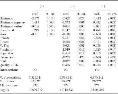
The estimation results of the nested logit model are presented in Table 3. The first column, model (a), displays the results of the estimation of a nested logit model where the specification includes only the variables of main interest: the geographical distance, its square and its cube (see the discussion following definition (2) in Section 3), the university standard and tuition fees. In model (b), we add to the specification of the nested logit model the control variables that characterize universities and the province they are located in. Model (c) adds to the specification of model (b) interaction terms between the three terms for geographical distance, university standard, and tuition fees and the student’s characteristics, that are the four cat-egorical variables presented in Section 4 (father’s occupation, mother’s education, secondary school type and final grade). The reference individual is a secondary school leaver coming from

14

For further information see, in Italian, “http://www.repubblica.it/speciale/2003/universita/indicatori.html”. 15

Descriptive statistics for the control variables are available in a previous version of this paper,Staffolani and

(13)

a family where the father’s occupation is blue-collar, whose mother education is primary school, graduated in a vocational school with a grade in the first quartile. Therefore, in model (c), the estimated coefficients associated with distance, standard, and fees apply to students with the reference characteristics. Let us call them the “weakest” students.

The second part of Table3 presents the dissimilarity parameters for the four field of studies while the dissimilarity parameter for the non-enrollment option, as a degenerate nest, must be normalized to 1 for identification. The third part of the table shows, among other information, the Likelihood–Ratio test for the IIA assumption: in the three cases, the null hypothesis of independence between alternatives is strongly rejected, which confirms the choice of estimating a the nested logit over a conditional logit model based on the bottom-level alternatives. The results of the estimation of the three conditional logit models corresponding to specifications (a), (b), and (c) are reported in the Appendix.

The coefficients associated with the geographical distance, its square and its cube imply a decreasing relationship (convex up to a distance of about 500 Km and then concave) between the distance and the choice probability and they do not vary significantly across the three models. This result can reasonably describe the behavior of Italian secondary school leavers: it may be conjectured that a student is more likely to enroll in a university close to home. The probability of choosing a university located in other provinces decreases in the cost and time of commuting; however, for those universities located too far to even commute, the decreasing effect on the choice probability attenuates. This is probably due to moving and renting costs being somewhat constant: it makes sense that transportation and renting costs may not be extremely different for various distances once the student has decided to move in order to attend university.

In all the three models tuition fees reduce the choice probability whereas higher university standards increase it. Once control variables are accounted for, as in model (b), a slightly difference in the coefficients for fees and standard emerge, whereas we obtain a remarkably higher value (in absolute value) of the coefficients for both standard and fees in model (c), where we explicitly consider individual heterogeneity: the weakest student and the average student are differently affected in the choice of university by the university standard and tuition fees. As expected, an increase in fees reduces the choice probability more for the weakest individual than for the average individuals. Instead, standards increase the choice probability more for the weakest student than for the average student. It may be conjectured that weaker students, holding fees constant, may seek out higher standards in order to compensate their poorer secondary school background and, therefore, increase their probability of getting a higher wage rate on the labor market. This aspect, will be discussed more in detail in Section 5.2 through the computation of elasticities for different classes of individuals.

As for the control variables, model (b) and (c) of Table 3 show that the coefficients of the closed and proximity dummies, and of the control variables of the location characteristics all have the expected sign. The coefficients of the dummy for private university and the number of faculties change sign between model (b) and model (c), where individual heterogeneity is taken into account. As opposed to the average student described in model (b), the weakest student is less likely to enroll in a private university (as expect, because higher tuition fees are usually charged by private universities) and prefers to enroll in universities with a high number of faculties.

5.2 Policy analysis: heterogeneous responses to supply-side variations

(14)

[image:14.595.85.512.175.611.2]

Table 3: Estimation results: nested logit model

(a) (b) (c)

coef. st. err. coef. st. err. coef. st. err.

Distance -2.703 (.048) -3.201 (.052) -3.571 (.111)

Distance square 0.374 (.008) 0.421 (.010) 0.500 (.031)

Distance cube -0.016 (.000) -0.018 (.000) -0.022 (.002)

Standard 0.198 (.003) 0.171 (.017) 0.818 (.002)

Fees -0.101 (.014) -0.132 (.004) -0.561 (.010)

Private 0.140 (.060) -0.554 (.068)

Closed -0.714 (.027) -0.567 (.027)

N. Fac. -0.019 (.002) 0.039 (.002)

Proximity 2.225 (.051) 1.369 (.050)

Population 0.453 (.014) 0.331 (.014)

Unem. rate -11.19 (.543) -9.218 (.526)

Rent -0.026 (.002) -0.006 (.002)

Quality of life 0.386 (.045) 0.348 (.044)

Interactions No No Yes

Dissimilarity parameters

Scientific 0.900 (.017) 1.128 (.017) 1.061 (.017)

Medical 0.774 (.016) 1.033 (.018) 0.944 (.017)

Social sciences 1.013 (.018) 1.229 (.017) 1.150 (.017)

Humanities 0.876 (.017) 1.105 (.017) 1.035 (.017)

Non enrollment 1 1 1

N. observations 6,875,344 6,875,344 6,875,344

N. of cases 25,277 25,277 25,277

Alt. per case 272 272 272

Log-lik -70119.383 -66478.636 -62308.328

LR test for IIA:χ2₄ 975.18, p-value=0.00 515.21,p-value=0.00 411.07,p-value=0.00

(15)

Table 4 shows the marginal effects, computed as in equation (6), of distance standard and tuition fees on the probability estimated using specification (c) by students characteristics. The computational intensive nature of the nested logit model estimation make the calculation of bootstrap standard errors for the marginal effects unfeasible. We, therefore, only show the results of diagnostic tests for the interaction coefficients summarized in Table 5.

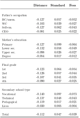
Table 4shows that the “weakest” students tend to choose universities closer to their home residence. The negative effect of geographical distance also significantly diminishes for increasing levels of the mother’s education, final secondary school grade, and for difficulty of secondary school type (see Table5). The marginal effects of standards reflect the results of the comparison between model (b) and (c): weaker students tend to seek out institution with higher standards although the marginal effect for wealthier and more talented students are rather small. The effect of tuition fees are negative and significantly increasing (in absolute value) for the “weakest” students suggesting a crucial role of financial constraints in the choice of university with respect to the cost charge by the institutions.

We also computed elasticities as per equation (7) with respect to distance, standard, and fees. We report the results in Figure 1 where we plot the elasticities to fees and standard as functions of the enrollment probability by students’ characteristics. For brevity, we do not plot the elasticities to distance as they show a very similar pattern to those to tuition fees.

Weaker students have a more evenly distributed probability of enrollment between 0 and 1 while wealthier (WC, CEO, degree) and more talented students (3rd and 4th quartile, Pedagog-ical and Liceo) present a higher enrollment probability. The latter group, therefore, has lower elasticities (in absolute value) to both standard and fees: if the enrollment probability is al-ready high, changes in the university attributes mildly affect such probability. On the contrary, such variations have a much greater effect on those students that are more subject to financial constrains and that have a weaker secondary school background.

To give a more precise idea of the values of these elasticities, Tables 6, 7, and 8 show the values of elasticities to distance, standard, and fees by sub-groups of individuals.

The elasticity to distance increases form −2.98% for students coming from a Vocational school with a low secondary school final grade to −0.08% for students coming from Liceo with a high secondary school grade (see Table 6). It means that, on average, living 10km further away form the closest university reduces the enrollment probability of an amount that ranges from 35% for the weakest students to 0.5% for students that are more talented and come from Liceo16. The considerable reduction of the probability for weaker students probably depends on the steeper negative slope in the relationship between probability and distance when distance tends to zero. A small distance identifies stayer students: therefore, on average, stayers should be weaker than movers.17

Students coming from Vocational schools and whose mother have a primary school title are those how seek the most universities with a high standard. Their elasticity to the university standard is almost 4.5% compared to an elasticity equal to 0 for Liceo graduates with the highest grades (see Table 7). More talented students already have an extremely high probability of enrolling (see also Figure 1) which may make them rather insensitive to small changes in the university standards.

Table 8 shows that modifying the level of the charged tuition fees changes considerably the composition of enrolled students in a given university. A increase of 100 Euros in the

16

Very similar results apply to students coming from Liceo whose mother is graduated or whose father is CEO, independently on the grade at secondary school.

17

(16)

[image:16.595.161.438.226.633.2]

yearly fees reduces the enrollment probability by 44.6% for the weaker students, while it has a remarkably decreasing effects for more talented and wealthier students to no effect at all for Liceo graduates with the highest grades. It is worth noticing that an increase in tuition fees penalizes more students with the highest secondary school grade and a mother whose educational level is primary or lower secondary (elasticity of−1.19% and−0.66% respectively) than students with a low secondary school grade and a graduated mother (elasticity of −0.50%). With respect to the willingness to pay for tuition fees, students seem to differ more according to the level of education of their mother than to the job position of their father.

Table 4: Direct marginal effects of distance, standard, and fees by students’ characteristics

Distance Standard Fees

BC/unem. -0.127 0.057 -0.052

WC -0.103 0.039 -0.027

Self-em. -0.127 0.062 -0.043

CEO -0.081 0.025 -0.022

Primary -0.127 0.099 -0.064

Lower sec. -0.132 0.058 -0.049

Upper sec. -0.098 0.026 -0.027

Degree -0.054 0.017 -0.012

Final grade

1st -0.123 0.064 -0.054

2nd -0.126 0.057 -0.044

3rd -0.107 0.041 -0.035

4th -0.090 0.027 -0.025

Vocational -0.140 0.097 -0.073

Technical -0.137 0.048 -0.043

Pedagogical -0.119 0.017 -0.021

Liceo -0.030 0.005 -0.004

Total -0.112 0.047 -0.039

6 Discussion and final remarks

(17)

[image:17.595.80.518.110.434.2]

Table 5: Diagnostics tests for interaction coefficients

Distance Standard Fees

WC Self CEO WC Self CEO WC Self CEO

BC/unem. ** ns ns ns ns ns *** *** ***

WC – ** *** – ns ns – ns ***

Self-em. – – ns – – ns – – ***

Lower Upper Degree Lower Upper Degree Lower Upper Degree

Primary ns ** *** *** *** *** *** *** ***

Lower sec. – * *** – *** *** – *** ***

Upper sec. – – *** – – ns – – ns

Final grade

2nd 3rd 4th 2nd 3rd 4th 2nd 3rd 4th

1st *** *** *** ns *** *** *** *** ***

2nd – *** *** – ** *** – *** ***

3rd – – *** – – ns – – ***

Tec. Liceo Ped. Tec. Liceo Ped. Tec. Liceo Ped.

Vocational ns *** *** *** *** *** *** *** ***

Technical – *** *** – *** *** – *** ***

Liceo – – *** – – ns – – ***

Foe each variable of interest (columns), we report thep-value of a test of equality between interaction coefficients

within each categorical variable, for instance H0 :γ_BC/unemF ees =γ_{W C}F ees. For geographical distance, we compute

Wald tests using theχ2 statistic with 3 degrees of freedom. For standard and fees, Wald tests using theχ21 are

computed, expect for comparisons with reference categories (BC/unem., Primary, 1st, and Vocational) for which

we report thep-value of thez-tests.

*p-value<0.10, **p-value<0.05, ***p-value<0.01, and nsp-value>0.10.

Table 6: Elasticities of the enrollment probability to distance, by students’ characteristics

Voc. Tec. Liceo Ped. 1st 2nd 3rd 4th Prim. Low. sec. Upp. sec. Degree

BC/unem. -2.66 -1.64 -0.29 -1.25 -2.20 -2.13 -1.55 -1.22 -2.25 -1.90 -1.28 -0.83

WC -2.17 -1.19 -0.18 -0.86 -1.50 -1.36 -0.92 -0.60 -1.81 -1.47 -0.90 -0.59

Self-em. -2.59 -1.65 -0.29 -1.11 -2.12 -2.00 -1.39 -1.10 -2.08 -1.92 -1.12 -0.71

CEO -2.09 -1.06 -0.12 -0.69 -1.14 -0.93 -0.65 -0.40 -1.77 -1.33 -0.67 -0.36

Primary -2.84 -1.89 -0.41 -1.64 -2.51 -2.56 -1.91 -1.59

Low. sec. -2.64 -1.66 -0.30 -1.23 -2.21 -2.08 -1.56 -1.20

Upp. sec. -2.10 -1.11 -0.16 -0.77 -1.36 -1.22 -0.78 -0.56

Degree -1.73 -0.84 -0.10 -0.59 -0.78 -0.59 -0.37 -0.20

1st -2.98 -1.99 -0.36 -1.59

2nd -2.83 -1.73 -0.22 -1.22

3rd -2.23 -1.12 -0.12 -0.75

[image:17.595.71.562.568.732.2]

(18)

[image:18.595.77.520.130.444.2]

Figure 1: Elasticities of the enrollment probability of to standard and fees, by students’ char-acteristics −5 0 5 10 −5 0 5 10

0 .5 1 0 .5 1

BC/unem. WC

Self−em. CEO

Elasticity to fees Elasticity to standards

Elasticities

Probability of Enrollment Father’s occupation −5 0 5 10 −5 0 5 10

0 .5 1 0 .5 1

Primary Lower sec.

Upper sec. Degree

Elasticities

Probability of Enrollment Mother’s education −5 0 5 10 −5 0 5 10

0 .5 1 0 .5 1

1st 2nd

3rd 4th

Elasticities

Probability of Enrollment Final grade −5 0 5 10 −5 0 5 10

0 .5 1 0 .5 1 Vocational Technical

Liceo Pedagogical

Elasticities

Probability of Enrollment

The solid and dashed lines are quadratic fits of the elasticities to fees and standards respectively.

Table 7: Elasticities of the enrollment probability to standard, by students’ characteristics

BC/unem. 3.09 1.05 0.09 0.37 2.33 1.86 1.25 0.79 2.93 1.54 0.71 0.54

WC 2.56 0.73 0.05 0.20 1.42 1.07 0.65 0.30 2.54 1.29 0.55 0.50

Self-em. 3.12 1.11 0.10 0.43 2.16 1.81 1.19 0.81 2.91 1.62 0.75 0.59

CEO 2.29 0.57 0.02 0.12 0.96 0.65 0.37 0.14 2.34 1.04 0.33 0.21

Primary 4.46 2.05 0.32 1.24 3.79 3.25 2.49 1.79

Low. sec. 2.87 0.99 0.10 0.34 2.19 1.71 1.15 0.70

Upp. sec. 2.00 0.45 0.02 0.06 0.99 0.74 0.36 0.16

Degree 2.23 0.55 0.03 0.15 0.67 0.42 0.21 0.06

1st 4.16 1.65 0.16 0.77

2nd 3.24 1.06 0.06 0.35

3rd 2.39 0.54 0.01 0.07

[image:18.595.71.547.549.712.2]

(19)

[image:19.595.72.565.96.260.2]

Table 8: Elasticities of the enrollment rate to tuition fees, by students’ characteristic

BC/unem. -2.53 -1.05 -0.10 -0.51 -2.04 -1.57 -1.14 -0.77 -2.07 -1.45 -0.84 -0.51

WC -1.72 -0.53 -0.02 -0.17 -1.03 -0.71 -0.44 -0.21 -1.40 -0.88 -0.42 -0.29

Self-em. -2.13 -0.81 -0.07 -0.35 -1.58 -1.22 -0.83 -0.57 -1.69 -1.18 -0.62 -0.39

CEO -1.75 -0.53 -0.02 -0.18 -0.82 -0.51 -0.32 -0.15 -1.46 -0.85 -0.34 -0.16

Primary -2.96 -1.39 -0.18 -0.87 -2.62 -2.11 -1.64 -1.19

Low. sec. -2.32 -0.94 -0.09 -0.43 -1.87 -1.40 -1.01 -0.66

Upp. sec. -1.70 -0.52 -0.03 -0.18 -0.94 -0.66 -0.39 -0.21

Degree -1.52 -0.41 -0.02 -0.14 -0.50 -0.28 -0.15 -0.05

1st -3.24 -1.45 -0.14 -0.78

2nd -2.42 -0.88 -0.05 -0.37

3rd -1.86 -0.53 -0.01 -0.16

4th -1.47 -0.33 -0.00 -0.07

and the socio-economic condition of her/his family of origin. Higher education choices are of great interest in Italy, where both participation and graduation rates are lower than the OECD average and where recent reforms have deeply modified the university system and have prompted a very comprehensive and vigorous debate.

Grounding the empirical analysis on a simple theoretical framework where secondary school leavers can be financially constrained both in the participation decision and in the choice of which university to attend, we derive a Random Utility Model that we trust is best estimated by a nested logit model. In order to highlight the relevance of individual characteristics, we interact the regressors of interest, that are geographical distance, tuition fees and university standard with categorical variables for family background (father’s occupation and mother’s level of education) and for the previous scholastic attainment (type of secondary school and final grade). The dataset used in our study, mainly based on the ISTAT national survey on secondary school leavers and from administrative databases of the Italian Ministry of Education, has a unique level of detail and has never been employed for this purpose.

The results of the nested logit model estimation confirm the prediction of our theoretical framework and mirror closely the findings related to other countries. The elasticity of the choice probability to geographical distance is, on average, −0.18%, the one to tuition fees is

−0.55%, and the one to university standards is 0.71%. These elasticities vary strongly among sub-groups of students, ranging from −0.08% to −2.98% for the geographical distance, from 0% to−3.24% for the university standard, and from −0.02% to 4.46% for tuition fees. Weaker students, that are those characterized by a family of origin with unfavored job positions and low educational attainment as well as by a diploma in vocational or technical schools and low secondary school grades, are more sensitive to changes in distance, fees and standards. Students coming from Liceo and with a favored family background (stronger students) have a high enrollment probability and exhibit smaller changes in their choice probabilities to variations of universities attributes .

(20)

a poor socio-economic condition of the household and scholastic background need to signal their university degree more strongly than favored students: moving and paying fees is costly, choosing a high ranked university is not ceteris paribus. According to the ideas behind our theoretical framework, this choice simply implies a lower probability of graduation and a higher expected earning for graduates, so a riskier option. It seems that weaker secondary school leavers are less risk adverse than more favored students.

The policy implications of our results are straightforward: every policy aimed to change tuition fees, as well as decisions of opening or closing universities or faculties, leads to conse-quences in term of enrollment probability that are stronger for students coming from families with a poor socio-economic background and with a diploma obtained in vocational or technical secondary schools. For instance, an increase in tuition fees of a 100 Euros reduces the enroll-ment probability of the weakest secondary school leavers by 44.6% and does not affect at all the enrollment rate of the strongest ones.

Given the ongoing financial crisis, governments and higher education institutions are likely to be financially constrained in many European countries and an economical/political debate has emerged (see Ichino and Terlizzese (2013) for Italy) aimed to find new solutions to the financing of higher education systems. The simplest way of facing such constraints is to raise tuition fees and reduce the territorial dispersion of academic institutions. As shown in our paper, this policies would have relevant consequences for the enrollment decisions of weaker students without affecting the choices of favored ones, and could further reduce the intergenerational mobility in education. Nevertheless, increasing the university quality, that is the effectiveness of universities in creating well remunerated human capital, will benefit more weaker students.

Further developments of the paper must firstly take into account students’ commitment during the studies and their probability of graduation, as they both depend on the students’ self–sorting process across different university attributes, that influence the university policy and the whole economy payoff. Then, in order to decide if some optimal university policy exists, some utility function of the university’s management and of the government must be considered.

References

Agasisti, T., and A. Dal Bianco (2007): “Determinants of college students migration in Italy: empirical evidence from a gravity approach,” Paper presented at the Congress of the European Regional Science Association, Paris.

Alm, J., and J. V. Winters (2009): “Distance and intrastate college student migration,” Economics of Education Review, 28(6), 728–738.

Cameron, A. C.(2005): Microeconometrics: methods and applications. Cambridge university press.

Cesi, B., and D. Paolini (2011): “University choice, peer group and distance,” Discussion paper, CRENoS.

Checchi, D., C. V. Fiorio, and M. Leonardi (2013): “Intergenerational persistence of educational attainment in Italy,” Economics Letters, 118(1), 229–232.

(21)

Drewes, T., andC. Michael(2006): “How Do Students Choose a University?: An Analysis of Applications to Universities in Ontario, Canada,” Research in Higher Education.

Frenette, M.(2004): “Access to College and University: Does Distance to School Matter?,” Canadian Public Policy, 30(4), 427–443.

(2006): “Too Far to Go On? Distance to School and University Participation,” Edu-cation Economics, 14(1), 31–58.

Gibbons, S., and A. Vignoles (2012): “Geography, choice adn participation in higher edu-cation in England,” Regional Science and Urban Economics, 42, 98–113.

Ichino, A., and D. Terlizzese (2013): Facolt`a di scelta. Rizzoli.

Long, B. T. (2004): “How have college decisions changed over time? An application of the conditional logistic choice model,”Journal of Econometrics, 121(1-2), 271–296.

Manski, C., and D. Wise (1983): College Choice in America. Harvard University Press, Cambridge.

OECD (2011): “Education at a Glance,” OECD Indicators.

Ordine, P., and C. Lupi (2009): “Family Income and Students’ Mobility,” Giornale degli Economisti, 68(1), 1–23.

S´a, C., R. J. Florax, and P. Rietveld (2004): “Does Accessibility to Higher Education matter? Choice Behavior of High School Graduates in the Netherlands,” Tinbergen Institute Discussion Papers 3, Tinbergen Institute.

Spiess, C. K., andK. Wrohlich(2010): “Does distance determine who attends a university in Germany?,” Economics of Education Review, 29(3), 470–479.

Staffolani, S., and C. Pigini(2012): “Enrolment Decision and University Choice of Italian Secondary School Graduates,” Working Papers 380, Universita’ Politecnica delle Marche (I), Dipartimento di Scienze Economiche e Sociali.

(22)

[image:22.595.95.505.142.471.2]