Compressed dynamic mode decomposition for background modeling

O R I G I N A L R E S E A R C H P A P E R

Compressed dynamic mode decomposition for background

modeling

N. Benjamin Erichson1 •_{Steven L. Brunton}2•_{J. Nathan Kutz}3

Received: 26 December 2015 / Accepted: 15 November 2016

ÓThe Author(s) 2016. This article is published with open access at Springerlink.com

Abstract We introduce the method of compressed dynamic mode decomposition (cDMD) for background modeling. The dynamic mode decomposition is a regres-sion technique that integrates two of the leading data analysis methods in use today: Fourier transforms and singular value decomposition. Borrowing ideas from compressed sensing and matrix sketching, cDMD eases the computational workload of high-resolution video process-ing. The key principal of cDMD is to obtain the decom-position on a (small) compressed matrix representation of the video feed. Hence, the cDMD algorithm scales with the intrinsic rank of the matrix, rather than the size of the actual video (data) matrix. Selection of the optimal modes characterizing the background is formulated as a sparsity-constrained sparse coding problem. Our results show that the quality of the resulting background model is competi-tive, quantified by the F-measure, recall and precision. A graphics processing unit accelerated implementation is also presented which further boosts the computational perfor-mance of the algorithm.

Keywords Dynamic mode decompositionBackground modelingMatrix sketching Sparse coding

GPU-accelerated computing

1 Introduction

One of the fundamental computer vision objectives is to detect moving objects in a given video stream. At the most basic level, moving objects can be found in a video by removing the background. However, this is a challenging task in practice, since the true background is often unknown. Algorithms for background modeling are required to be both robust and adaptive. Indeed, the list of challenges is significant and includes camera jitter, illu-mination changes, shadows and dynamic backgrounds. There is no single method currently available that is cap-able of handling all the challenges in real time without suffering performance failures. Moreover, one of the great challenges in this field is to efficiently process high-reso-lution video streams, a task that is at the edge of perfor-mance limits for state-of-the-art algorithms. Given the importance of background modeling, a variety of mathe-matical methods and algorithms have been developed over the past decade. Comprehensive overviews of traditional and state-of-the-art methods are provided by Bouwmans [1], and Sobral and Vacavant [2].

MotivationThis work advocates the method of dynamic mode decomposition (DMD), which enables the decom-position of spatiotemporal grid data in both space and time. The DMD has been successfully applied to videos [3–5]; however, the computational costs are dominated by the singular value decomposition (SVD). Even with the aid of recent innovations around randomized algorithms for computing the SVD [6], the computational costs remain expensive for high-resolution videos. Importantly, we build on the recently introduced compressed dynamic mode decomposition (cDMD) algorithm, which integrates DMD with ideas from compressed sensing and matrix sketching [7]. Hence, instead of computing the DMD on the

full-& N. Benjamin Erichson [email protected]

1 _{School of Mathematics and Statistics, University of St} Andrews, St Andrews, United Kingdom

2 _{Department of Mechanical Engineering, University of} Washington, Seattle, WA 98195, USA

resolution video data, we show that an accurate decom-position can be obtained from a compressed representation of the video in a fraction of the time. The optimal mode selection for background modeling is formulated as a sparsity-constrained sparse coding problem, which can be efficiently approximated using the greedy orthogonal matching pursuit method. The performance gains in com-putation time are significant, even competitive with Gaussian mixture models [8–11]. Moreover, the perfor-mance evaluation on real videos shows that the detection accuracy is competitive compared to leading robust prin-cipal component analysis (RPCA) algorithms.

OrganizationThe rest of this paper is organized as fol-lows. Section2presents a brief introduction to the dynamic mode decomposition and its application to video and back-ground modeling. Section3presents the compressed DMD algorithm and different measurement matrices to construct the compressed video matrix. A GPU-accelerated imple-mentation is also outlined. Finally a detailed evaluation of the algorithm is presented in Sect.4. Concluding remarks and further research directions are given in Sect.5. ‘‘Appendix’’ gives an overview of notation.

2 DMD for video processing

2.1 The dynamic mode decomposition

The dynamic mode decomposition is an equation-free, data-driven matrix decomposition that is capable of providing accurate reconstructions of spatiotemporal coherent struc-tures arising in nonlinear dynamical systems, or short-time future estimates of such systems. DMD was originally introduced in the fluid mechanics community by Schmid [12] and Rowley et al. [13]. A surveillance video sequence offers an appropriate application for DMD because the frames of the video are, by nature, equally spaced in time, and the pixel data, collected in every snapshot, can readily be

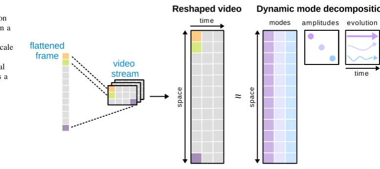
vectorized. The dynamic mode decomposition is illustrated for videos in Fig.1. For computational convenience, the flattened grayscale video frames (snapshots) of a given video stream are stored, ordered in time, as column vectors

x1;x2;. . .;xmof a matrix. Hence, we obtain a 2-dimensional

Rnm _{spatiotemporal grid, wheren denotes the number of}

pixels per frame,mis the number of video frames taken, and the matrix elements xit correspond to a pixel intensity in

space and time. The video frames can be thought of as snapshots of some underlying dynamics. Each video frame (snapshot)xtþ1at timetþ1 is assumed to be connected to the previous framextby a linear mapA:Rn!Rn.

Math-ematically, the linear mapAis a time-independent operator which constructs the approximate linear evolution

xtþ1 ¼Axt: ð1Þ

The objective of dynamic mode decomposition is to find an estimate for the matrixAand its eigenvalue decomposition that characterizes the system dynamics. At its core, dynamic mode decomposition is a regression algorithm. First, the spatiotemporal grid is separated into two overlapping sets of data, called the left and right snapshot sequences

X=

⎡

⎣x1x2· · · xm−1

⎤ ⎦, X=

⎡

⎣x2x3· · · xm ⎤

⎦. ð2Þ

Equation (1) is reformulated in matrix notation

X0¼AX: ð3Þ

In order to find an estimate for the matrix Awe face the following least-squares problem

^

A¼argmin

A

kX0AXk2F; ð4Þ

where k kF denotes the Frobenius norm. This is a

well-studied problem, and an estimate of the linear operatorAis given by

Fig. 1 Illustration of the dynamic mode decomposition for video applications. Given a video stream, the first step involves reshaping the grayscale video frames into a

^

A¼X0Xy; ð5Þ

whereydenotes the Moore-Penrose pseudoinverse, which produces a regression that is optimal in a least-square sense. The DMD modes U¼W, containing the spatial information, are then obtained as eigenvectors of the matrixA^

^

AW¼WK; ð6Þ

where columns of W are eigenvectors /j and K is a

diagonal matrix containing the corresponding eigenvalues kj. In practice, when the dimensionn is large, the matrix

^

A2Rnn _{may be intractable to estimate and to analyze}

directly. DMD circumvents the computation ofA^ by con-sidering a rank-reduced representation A~2Rkk. This is achieved by using the similarity transform, i.e., projecting

^

Aon the left singular vectors. Moreover, DMD typically makes use of the low-rank structure so that the total number of modes,kminðn;mÞ, allows for dimensionality reduction of the video stream. Hence, only the relatively smallA~2Rkkmatrix needs to be estimated and analyzed (see Sect.3 for more details). The dynamic mode decom-position yields the following low-rank factorization of a given spatiotemporal grid (video stream)

UBV ¼

/11 /1p /1k .. . .. . . . . .. .

/i1 /ip /ik .. . .. . . . . .. .

/n1 /np /nk 0 B B B B B B B B @ 1 C C C C C C C C A b1 . . . bp . . . bk 0 B B B B B B B B @ 1 C C C C C C C C A

1 k1 km11

.. . .. . . . . .. .

1 kp kmp1 .. . .. . . . . .. .

1 kk kmk1 0 B B B B B B B B @ 1 C C C C C C C C A ; ð7Þ

where the diagonal matrixB2Ckkhas the amplitudes as entries andV 2Ckmis the Vandermonde matrix describing the temporal evolution of the DMD modesU2Cnk.

2.2 DMD for foreground/background separation

The DMD method can attempt to reconstruct any given frame, or even possibly future frames. The validity of the reconstruction thereby depends on how well the specific video sequence meets the assumptions and criteria of the DMD method. Specifically, a video framextat time points

t21;. . .;mis approximately reconstructed as follows

~ xt¼

Xk

j¼1 bj/jk

t1

j : ð8Þ

Notice that the DMD mode/jis an1 vector containing

the spatial structure of the decomposition, while the eigenvalue ktj1 describes the temporal evolution. The

scalarbjis the amplitude of the corresponding DMD mode.

At timet¼1, Eq. (8) reduces tox~1¼P

k

j¼1bj/j. Since the

amplitude is time-independent, bj can be obtained by

solving the following least-square problem using the video framex1 as initial condition

^

b¼argmin

b

kx1Ubk 2

F: ð9Þ

It becomes apparent that any portion of the first video frame that does not change in time, or changes very slowly in time, must have an associated continuous-time eigenvalue

xj¼

logðkjÞ

Dt ð10Þ

that is located near the origin in complex space:jxjj 0 or

equivalentjkjj 1. This fact becomes the key principle to

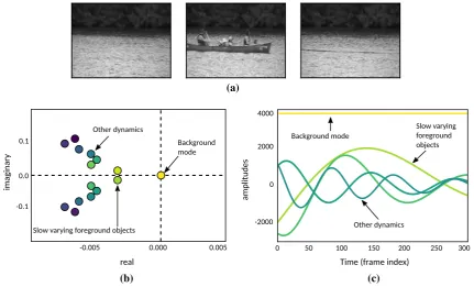
separate foreground elements (approximate sparse) from background (approximate low-rank) information. Figure2 shows the dominant continuous-time eigenvalues for a video sequence. Subplot (a) shows three sample frames from this video sequence that includes a canoe. Here the foreground object (canoe) is not present at the beginning and the end for the video sequence. The dynamic mode decomposition factorizes this sequence into modes describing the different dynamics present. The analysis of the continuous-time eigenvaluexjand the amplitudes over

matrix decompositions. Following this approach, back-ground modeling can be formulated as a matrix separation problem into low-rank (background) and sparse (fore-ground) components. This viewpoint has been advocated, for instance, by Cande`s et al. [14] in the framework of robust principal component analysis (RPCA). For a thor-ough discussion of such methods used for background modeling, we refer to Bouwmans et al. [15, 16]. The connection between DMD and RPCA was first established by Grosek and Kutz [3]. Assume the set of background modes fxpg satisfies jxpj 0. The DMD expansion of

Eq. (8) then yields

XDMD¼LþS ¼X

p

bp/pk t1

p

|fflfflfflfflfflfflfflfflffl{zfflfflfflfflfflfflfflfflffl}

BackgroundVideo þX

j6¼p

bj/jk t1

j

|fflfflfflfflfflfflfflffl{zfflfflfflfflfflfflfflffl}

ForegroundVideo

; _ð11Þ

where t¼ ½1;. . .;m is a 1m time vector and

XDMD 2Cnm.1 Specifically, DMD provides a matrix decomposition of the formXDMD¼LþS, where the

low-rank matrixLwill render the video of just the background,

and the sparse matrix S will render the complementary video of the moving foreground objects. We can interpret these DMD results as follows: Stationary background objects translate into highly correlated pixel regions from one frame to the next, which suggests a low-rank structure within the video data. Thus, the DMD algorithm can be thought of as an RPCA method. The advantage of the DMD method and its sparse/low-rank separation is the computational efficiency of achieving Eq. (11), especially when compared to the optimization methods of RPCA. The analysis of the time evolving amplitudes provides inter-esting opportunities. Specifically, learning the amplitudes’ profiles for different foreground objects allows automatic separation of video feeds into different components. For instance, it could be of interest to discriminate between cars and pedestrians in a given video sequence.

2.3 DMD for real-time background modeling

When dealing with high-resolution videos, the standard DMD approach is expensive in terms of computational time and memory, because the whole video sequence is reconstructed. Instead a ‘good’ static background model is often sufficient for background subtraction. This is because background dynamics can be filtered out or thresholded. (a)

(b) (c)

Fig. 2 Results of the dynamic mode decomposition for the ChangeDetection.net video sequence ‘canoe’. Subplotashows three samples frames of the video sequence. Subplotsband cshow the continuous-time eigenvalues and the temporal evolution of the amplitudes. The modes corresponding to the amplitudes with the highest variance are capturing the dominant foreground object

(canoe), while the zero mode is capturing the dominant structure of the background. Modes corresponding to high-frequency amplitudes capturing other dynamics in the video sequence, e.g., waves.aSample frames (t¼0;150;300) of video sequence.bDominant continuous-time eigenvaluesxj.cAmplitudes over time

1 _{Note that by constructionX}

The challenge remains to automatically select the modes best describing the background. This is essentially a bias-variance trade-off. Using just the zero mode (background) leads to an under-fitted background model, while a large set of modes tends to overfit. Motivated, by the sparsity-promoting variant of the standard DMD algorithm intro-duced by Jovanovic´ et al. [17], we formulate a sparsity-constrained sparse coding problem for mode selection. The idea is to augment Eq. (9) by an additional term that penalizes the number of nonzero elements in the vectorb

^

b¼argmin b

kx1Ubk2F such thatkbk0\K; ð12Þ

whereb is the sparse representation ofb, and k k0 is ‘0 pseudo-norm which counts the nonzero elements in b. Solving this sparsity problem exactly is NP-hard. However, the problem in Eq. (12) can be efficiently solved using greedy approximation methods. Specifically, we utilize orthogonal matching pursuit (OMP) [18, 19]. A highly computationally efficient algorithm is proposed by Rubin-stein et al. [20] and is implemented in the scikit-learn software package [21]. The greedy OMP algorithm works iteratively, selecting at each step the mode with the highest correlation to the current residual. Once a mode is selected, the initial condition x1 is orthogonally projected on the span of the previously selected set of modes. Then the residual is recomputed and the process is repeated untilK nonzero entries are obtained. If no priors are available, the optimal number of modesKcan be determined using cross-validation. Finally, the background model is computed as

^

xBG¼Ub:^ ð13Þ

3 Compressed DMD (cDMD)

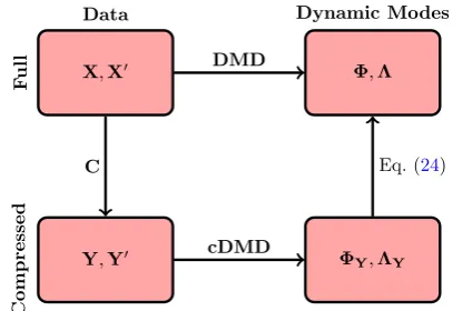
Compressed DMD provides a computationally efficient framework to compute the dynamic mode decomposition on massively under-sampled or compressed data [7]. The method was originally devised to reconstruct high-dimen-sional, full-resolution DMD modes from sparse, spatially under-resolved measurements by leveraging compressed sensing. However, it was quickly realized that if full-state measurements are available, many of the computationally expensive steps in DMD may be computed on a com-pressed representation of the data, providing dramatic computational savings. The first approach, where DMD is computed on sparse measurements without access to full data, is referred to ascompressed sensing DMD. The sec-ond approach, where DMD is accelerated using a combi-nation of calculations on compressed data and full data, is referred to ascompressed DMD(cDMD); this is depicted schematically in Fig.3. For the applications explored in

this work, we use compressed DMD, since full image data are available and reducing algorithm runtime is critical for real-time performance.

3.1 Compressed sensing and matrix sketching

Compression algorithms are at the core of modern video, image and audio processing software such as MPEG, JPEG and MP3. In our mathematical infrastructure of compressed DMD, we consider the theory of compressed sensing and matrix sketching.

Compressed sensing demonstrates that instead of mea-suring the high-dimensional signal, or pixel space repre-sentation of a single frame x, we can measure instead a low-dimensional subsampleyand approximate/reconstruct the full-state space x with this significantly smaller mea-surement [22–24]. Specifically, compressed sensing assumes the data being measured are compressible in some basis, which is certainly the case for video. Thus, the video can be represented in a small number of elements of that basis, i.e., we only need to solve for the few nonzero coefficients in the transform basis. For instance, consider the measurements y2Rp, withk\pn:

y¼Cx: ð14Þ

Ifxis sparse inW, then we may solve the underdetermined system of equations

y¼CWs ð15Þ

forsand then reconstructx. Since there are infinitely many solutions to this system of equations, we seek the sparsest solution^s. However, it is well known from the compressed sensing literature that solving for the sparsest solution

X,X Φ,Λ

Y,Y Φ_Y,Λ_Y

DMD

cDMD

C Eq. (24)

Data Dynamic Modes

F

ull

Compressed

formally involves an‘0 optimization that is NP-hard. The success of compressed sensing is that it ultimately engi-neered a solution around this issue by showing that one can instead, under certain conditions on the measurement matrixC, trade the infeasible‘0 optimization for a convex ‘1-minimization [22]:

^

s¼argmin

s0 k

s0k1; such thaty¼CWs 0_:

ð16Þ

Thus, ‘1-norm acts as a proxy for sparsity-promoting solutions ofs^. To guarantee that the compressed sensing architecture will almost certainly work in a probabilistic sense, the measurement matrixCand sparse basisWmust beincoherent, meaning that the rows ofCare uncorrelated with the columns ofW. This is discussed in more detail in [7]. Given that we are considering video frames, it is easy to suggest the use of generic basis functions such as Fourier or wavelets in order to represent the sparse signals. Indeed, wavelets are already the standard for image compression architectures such as JPEG-2000. As for the Fourier transform basis, it is particularly attractive for many engineering purposes since single-pixel measurements are clearly incoherent given that it excites broadband fre-quency content.

Matrix sketching is another prominent framework in order to obtain a similar compressed representation of a massive data matrix [25, 26]. The advantage of this approach is the less restrictive assumptions and the straight forward generalization from vectors to matrices. Hence, Eq. (14) can be reformulated in matrix notation

Y¼CX; ð17Þ

where again C denotes a suitable measurement matrix. Matrix sketching comes with interesting error bounds and is applicable whenever the data matrix X has low-rank structure. For instance, it has been successfully demon-strated that the singular values and right singular vectors can be approximated from such a compressed matrix rep-resentation [27].

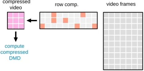
3.2 Algorithm

The compressed DMD algorithm proceeds similarly to the standard DMD algorithm [28] at nearly every step until the computation of the DMD modes. The key difference is that we first compute a compressed representation of the video sequence, as illustrated in Fig.4. Hence the algorithm starts by generating the measurement matrixC2Rpnin order to compresses or sketch the data matrices as in Eq. (2):

Y¼CX; Y0¼CX0: ð18Þ

Where p is denoting the number of samples or measure-ments. There is a fundamental assumption that the input

data are low-rank. This is satisfied for video data, because each of the columns of X and X02Rnm1 is sparse in some transform basis W. Thus, for sufficiently many incoherent measurements, the compressed matrices Yand

Y02Rpm1 _{have similar correlation structures to their} high-dimensional counterparts. Then compressed DMD approximates the eigenvalues and eigenvectors of the lin-ear mapAY, where the estimator is defined as:

^

AY¼Y0Yy ð19aÞ

¼Y0VYSY1UY; ð19bÞ

where denotes the conjugate transpose. The pseudo-inverse Yy is computed using the SVD:

Y¼UYSYVY; ð20Þ

where the matrices U2Rpk_{, and V2R}m1k _{are the}

truncated left and right singular vectors. The diagonal matrix S2Rkk has the corresponding singular values as entries. Here k is the target-rank of the truncated SVD approximation to Y. Note that the subscriptYis included to explicitly denote computations involving the com-pressed data Y. As in the standard DMD algorithm, we typically do not compute the large matrix A^Y, but instead

compute the low-dimensional model projected onto the left singular vectors:

~

AY¼UYA^YUY ð21aÞ

¼U_YY0VYSY1: ð21bÞ

Since this is a similarity transform, the eigenvectors and eigenvalues can be obtained from the eigendecomposition ofA~Y

~

AYWY¼WYKY; ð22Þ

UY¼Y0VYSY1WY: ð23Þ

Finally, the full DMD modes are recovered using

U¼X0VYSY1WY: ð24Þ

Note that the compressed DMD modes in Eq. (24) make use of the full dataX0as well as the linear transformations obtained using the compressed data Y and Y0. The expensive SVD on X is bypassed, and it is instead per-formed on Y. Depending on the compression ratio, this may provide significant computational savings. The com-putational steps are summarized in Algorithm 1, and fur-ther numerical details are presented in [7].

Remark 1 The computational performance heavily depends on the measurement matrix used to construct the compressed matrix, as described in the next section. For a practical implementation sparse or single-pixel measure-ments (random row selection) are favored.

Remark 2 One alternative to the predefined target-rank kis the recent hard-thresholding algorithm of Gavish and Donoho [29]. This method can be combined with step 4 to automatically determine the optimal target-rank.

Remark 3 As described in Sect.2.3, step 9 can be replaced by the orthogonal matching pursuit algorithm, in order to obtain a sparsity-constrained solution: b¼ompðU;x1Þ. Computing the OMP solution is in general extremely fast, but if it comes to high-resolution video streams this step can become computationally expensive. However, instead of computing the amplitudes based on the full-state dynamic modes U the compressed DMD modes UY can be used.

Hence, Eq. (12) can be reformulated as

^

b¼argmin b

ky₁UYbk2F such that kbk0\K; ð25Þ

wherey₁ is the first compressed video frame. Then step 9 can be replaced by:b¼ompðUY;y1Þ.

3.3 Measurement matrices

A basic measurement matrix C can be constructed by drawingpn independent random samples from a Gaus-sian, Uniform or a sub GausGaus-sian, e.g., Bernoulli distribu-tion. It can be shown that these measurement matrices have optimal theoretical properties; however, for practical large-scale applications they are often not feasible. This is because generating a large number of random numbers can be expensive and computing Eq. (18) using unstructured dense matrices has a time complexity of O(pnm). From a computational perspective, it is favorable to build a struc-tured random sensing matrix which is memory efficient and

enables the execution of fast matrix-matrix multiplications. For instance, Woolfe et al. [30] showed that the costs can be reduced to O(log(p)nm) using a subsampled random Fourier transform (SRFT) sensing matrix

C¼RFD; ð26Þ

where R2Cpn draws p random rows (without replace-ment) from the identity matrix I2Cnn.F2Cnn is the unnormalized discrete Fourier transform with the following entries Fðj;kÞ ¼expð2piðj1Þðk1Þ=mÞ, and D2

Cnn is a diagonal matrix with independent random diag-onal elements uniformly distributed on the complex unit circle. While the SRFT sensing matrix has nice theoretical properties, the improvement from O(pnm) to O(log(p)nm) Algorithm 1 Compressed Dynamic Mode Decomposition. Given a matrixD ∈ Rn×m containing the flattened

video frames, this procedure computes the approximate dynamic mode decomposition, whereΦ∈ Cn×k are the DMD modes, b ∈ Ck are the amplitudes, andV ∈ Ck×m is the Vandermonde matrix describing the temporal evolution. The procedure can be controlled by the two parametersk andp, the target rank and the number of samples respectively. It is required thatn≥m, integerk, p≥1 andkmandp≥k.

function[Φ,b,V] =cdmd(D, k, p)

(1) X,X=D Left/right snapshot sequence.

(2) C=rand(p, m) Drawp×msensing matrix.

(3) Y,Y=C∗D Compress input matrix.

(4) U,S,V=svd(Y, k) Truncated SVD.

(6) A˜=U∗∗Y∗V∗S−1 Least squares fit.

(7) W,Λ=eig(A˜) Eigenvalue decomposition.

(8) Φ←X∗V∗S−1∗W Compute full-state modesΦ.

(9) b=lstsq(Φ,x₁) Compute amplitudes usingx₁as intial condition.

is not necessarily significant. In practice, it is often suffi-cient to construct even simpler sensing matrices. An interesting approach making the matrix-matrix multiplica-tion in Eq. (18) redundant is to use single-pixel measure-ments (random row selection)

C¼R: ð27Þ

In a practical implementation, this allows construction of the compressed matrix Y from choosing p random rows without replacement fromX. Hence, only prandom num-bers need to be generated and no memory is required for storing a sensing matrix C. A different approach is the method of sparse random projections [31]. The idea is to construct a sensing matrix C with identical independent distributed entries as follows

cij¼

1 with prob. 1 2s 0 with prob. 11

s;

1 with prob. 1 2s 8

> > > > > < > > > > > :

ð28Þ

where the parameter s controls the sparsity. While Ach-lioptas [31] has proposed the valuess¼1;2, Li et al. [32] showed that also very sparse (aggressive) sampling rates likes¼n=logðnÞ achieve accurate results. Modern sparse matrix packages allow rapid execution of (18).

3.4 GPU-accelerated implementation

While most current desktop computers allow multi-threading and also multiprocessing, using a graphics processing unit (GPU) enables massive parallel pro-cessing. The paradigm of parallel computing becomes more important as larger amounts of data stagnate CPU clock speeds. The architecture of a modern CPU and GPU is illustrated in Fig.5. The key difference between these architectures is that the CPU consists of few arithmetic logic units (ALU) and is highly optimized for low-latency access to cached data sets, while the GPU is optimized for data-parallel, throughput computations. This is achieved by the large number of small arithmetic logic units (ALU). Traditionally, this architecture was designed for the real-time creation of high-definition 2D/ 3D graphics. However, NVIDIA’s programming model for parallel computing CUDA opens up the GPU as a general parallel computing device [33]. Using high-per-formance linear algebra libraries, e.g., CULA [34], can help to accelerate comparable CPU implementations substantially. Take for instance the matrix multiplication of two nn square matrices, illustrated in Fig.6. The computation involves the evaluation ofn2 dot products.2 The data parallelism therein is that each dot-product can

be computed independently. With enough ALUs the computational time can be substantially accelerated. This parallelism applies readily to the generation of random numbers and many other linear algebra routines.

Relatively, few GPU-accelerated background subtrac-tion methods have been proposed [11,35,36]. The authors achieve considerable speedups compared to the corre-sponding CPU implementations. However, the proposed methods barely exceed 25 frames per second for

high-(a) (b)

Fig. 5 Illustration of the CPU and GPU architecture.aCPU.bGPU

Fig. 6 Illustration of the data parallelism in matrix-matrix multiplications

definition videos. This is mainly due to the fact that many statistical methods do not fully benefit from the GPU architecture. In contrast, linear algebra-based methods can substantially benefit from parallel computing. An analysis of Algorithm 1 reveals that generating random numbers in line 2 and the dot products in lines 3, 6 and 8 is particularly suitable for parallel processing. But also the computation of the deterministic SVD, the eigenvalue decomposition and the least-square solver can benefit from the GPU archi-tecture. Overall, the GPU-accelerated DMD implementa-tion is substantially faster than theMKL(Intel Math Kernel Library) accelerated routine. The disadvantage of current GPUs is the rather limited bandwidth, i.e., the amount of data which can be exchanged per unit of time, between CPU and GPU memory. However, this overhead can be mitigated using asynchronous memory operations.

4 Results

In this section, we evaluate the computational performance and the suitability of compressed DMD for background modeling. To evaluate the detection performance, a fore-ground maskXis computed by thresholding the difference between the true frame and the reconstructed background. A standard method is to use the Euclidean distance, leading to the following binary classification problem

XtðjÞ ¼

1 if kxjtx^jk[s;

0 otherwise

ð29Þ

wherexjtdenotes thejth pixel of thetth video frame andx^j

denotes the corresponding pixel of the modeled background. Pixels belonging to foreground objects are set to 1 and 0 otherwise. Access to the true foreground mask allows the computation of several statistical measures. For instance, common evaluation measures in the background subtraction literature are recall, precision and the F-measure. While recall measures the ability to correctly detect pixels belonging to moving objects, precision measures how many predicted foreground pixels are actually correct, i.e., false alarm rate. The F-measure combines both measures by their harmonic mean. A workstation (Intel Xeon CPU E5-2620 2.4GHz, 32GB DDR3 memory and NVIDIA GeForce GTX 970) was used for all following computations.

4.1 Evaluation on real videos

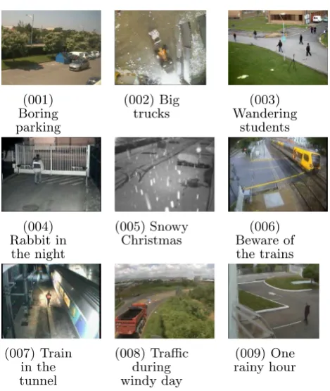
We have evaluated the performance of compressed DMD for background modeling using the CD (ChangeDetec-tion.net) and BMC (Background Models Challenge) benchmark dataset [37, 38]. Figure7 illustrates the nine real videos of the latter dataset, posing many common

challenges faced in outdoor video surveillance scenarios. Mainly, the following complex situations are encountered: – Illumination changes: Gradual illumination changes

caused by fog or sun.

– Low illumination: Bad light conditions, e.g., night videos.

– Bad weather: Introduced noise (small objects) by weather conditions, e.g., snow or rain.

– Dynamic backgrounds: Moving objects belonging to the background, e.g., waving trees or clouds.

– Sleeping foreground objects: Former foreground objects that becoming motionless and moving again at a later point in time.

Evaluation settings In order to obtain reproducible results the following settings have been used. For a given video sequence, the low-rank dynamic mode decomposi-tion is computed using a very sparse measurement matrix with a sparsity factor s¼n=logðnÞ and p¼1000 mea-surements. While, we use here a fixed number of samples, the choice can be guided by the formula p[klogðn=kÞ. The target-rank k is automatically determined via the optimal hard-threshold for singular values [29]. Once the dynamic mode decomposition is obtained, the optimal set of modes is selected using the orthogonal matching pursuit method. In general the use of K¼10 nonzero entries achieves good results. Instead of using a predefined value for K, cross-validation can be used to determine the

(001) Boring parking

(002) Big trucks

(003) Wandering

students

(004) Rabbit in

the night

(005) Snowy Christmas

(006) Beware of the trains

(007) Train in the tunnel

(008) Traffic during windy day

(009) One rainy hour

optimal number of nonzero entries. Further, the dynamic mode decomposition as presented here is formulated as a batch algorithm, in which a given long video sequence is split into batches of 200 consecutive frames. The decom-position is then computed for each batch independently.

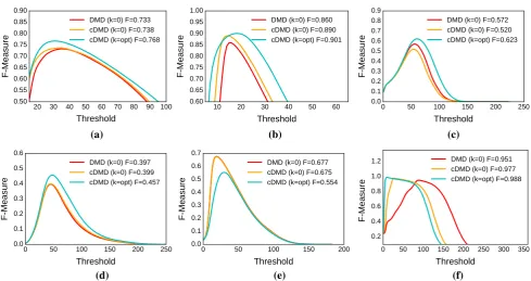
The CD datasetFirst, six CD video sequences are used to contextualize the background modeling quality using the sparse coding approach. This is compared to using the zero (static background) mode only. Figure8shows the evalu-ation results of one batch by plotting the F-measure against the threshold for background classification. In five out of six examples, the sparse coding approach (cDMD k=opt) dominates. In particular, significant improvements are achieved for the dynamic background video sequences ‘Canoe’ and ‘Fountain02’. Only in case of the ‘Park’ video sequence, the method tends to overfit. Interestingly, the performance of the compressed algorithm is slightly better than the exact DMD algorithm, overall. This is due to the implicit regularization of randomized algorithms [39,40]. The BMC dataset In order to compare the cDMD algorithm with other RPCA algorithms, the BMC dataset has been used. Table1 shows the evaluation results com-puted with the BMC wizard for all ninevideos. An indi-vidual threshold value has been selected for each video to compute the foreground mask. For comparison, the eval-uation results of three other RPCA methods are shown [16]. Overall, cDMD achieves an average F-value of about

0.648. This is slightly better than the performance of GoDec [41] and nearly as good as LSADM [42]. However, it is lower than the F-measure achieved with the RSL method [43]. Figure9 presents visual results for example frames across five videos. The last row shows the smoothed (median filtered) foreground mask.

Discussion The results reveal some of the strengths and limitations of the compressed DMD algorithm. First, because cDMD is presented here as a batch algorithm, detecting sleeping foreground objects as they occur in video 001 is difficult. Another weakness is the limited capability of dealing with non-periodic dynamic backgrounds, e.g., big waving trees and moving clouds as occurring in the videos 001, 005, 008 and 009. On the other hand, good results are achieved for the videos 002, 003, 004 and 007, showing that DMD can deal with large moving objects and low illumination conditions. The integration of compressed DMD into a video system can overcome some of these initial issues. Hence, instead of discarding the previous modeled background frames, a background mainte-nance framework can be used to incrementally update the model. In particular, this allows to deal better with sleeping foreground objects. Further, simple post-pro-cessing techniques (e.g., median filter or morphology transformations) can substantially reduce the false positive rate.

(a) (b) (c)

(d) (e) (f)

Fig. 8 The F-measure for varying thresholds is indicating the dominant background modeling performance of the sparsity-promot-ing compressed DMD algorithm. In particular, the performance gain

4.2 Computational performance

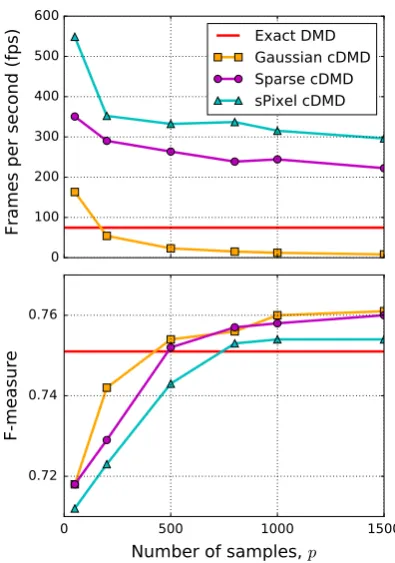
Figure10shows the fps rate and the F-measure for a varying number of samplespand different measurement matrices. Gaussian measurements achieve the best accuracy in terms of the F-measure, but the computational costs become increasingly expensive. Single-pixel measurements (sPixel) are the most computationally efficient method. The primary advantages of single-pixel measurements are the memory efficiency and the simple implementation. Sparse sensing matrices offer the best trade-off between computational time and accuracy, but require access to sparse matrix packages. It is important to stress that randomized sensing matrices cause random fluctuations influencing the background model quality, illustrated in Fig.11. The bootstrap

confidence intervals show that sparse measurements have lower dispersion than single-pixel measurements. This is, because single-pixel measurements discard more informa-tion than sparse and Gaussian sensing matrices.

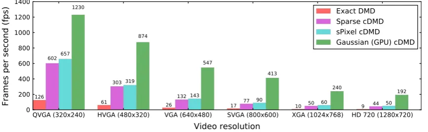
Figure12 shows the average frames per seconds (fps) rate required to obtain the foreground mask for varying video resolutions. The results illustrate the substantial Table 1 Evaluation results of nine real videos from the BMC dataset

Measure BMC real videos Average

001 002 003 004 005 006 007 008 009

RSL De La Torre et al. [43] Recall 0.800 0.689 0.840 0.872 0.861 0.823 0.658 0.589 0.690 –

Precision 0.732 0.808 0.804 0.585 0.598 0.713 0.636 0.526 0.625 –

F-Measure 0.765 0.744 0.821 0.700 0.706 0.764 0.647 0.556 0.656 0.707 LSADM Goldfarb et al. [42] Recall 0.693 0.535 0.784 0.721 0.643 0.656 0.449 0.621 0.701 –

Precision 0.511 0.724 0.802 0.729 0.475 0.655 0.693 0.633 0.809 –

F-Measure 0.591 0.618 0.793 0.725 0.549 0.656 0.551 0.627 0.752 0.650

GoDec Zhou and Tao [41] Recall 0.684 0.552 0.761 0.709 0.621 0.670 0.465 0.598 0.700 –

Precision 0.444 0.682 0.808 0.728 0.462 0.636 0.626 0.601 0.747 –

F-Measure 0.544 0.611 0.784 0.718 0.533 0.653 0.536 0.600 0.723 0.632

cDMD Recall 0.552 0.697 0.778 0.693 0.611 0.700 0.720 0.515 0.566 –

Precision 0.581 0.675 0.773 0.770 0.541 0.602 0.823 0.510 0.574 –

F-Measure 0.566 0.686 0.776 0.730 0.574 0.647 0.768 0.512 0.570 0.648

For comparison, the results of three other leading robust PCA algorihtms are presented, adapted from [16]. The best performing algorithm for each video has its table entries highlighted in bold

Fig. 9 Visual evaluation results for five example frames correspond-ing to the BMC videos: 002, 003, 006, 007 and 009. Thetop row

shows the original grayscale images (moving objects arehighlighted). Thesecond row shows the differencing between the reconstructed cDMD background and the original frame. Row three shows the thresholded androw fourthe in addition median filtered foreground mask

computational advantage of the cDMD algorithm over the standard DMD. The computational savings are mainly achieved by avoiding the expensive computation of the singular value decomposition. Specifically, the compres-sion step reduces the time complexity from O(knm) to O(kpm). The computation of the full modes U in Eq.24 remains the only computational expensive step of the algorithm. However, this step is embarrassingly parallel and the computational time can be further reduced using a GPU-accelerated implementation. The decomposition of a HD 1280720 videos feed using the GPU-accelerated implementation achieves a speedup of about 4 and 21 compared to the corresponding CPU cDMD and (exact) DMD implementations. The speedup of the GPU imple-mentation can even further be increased using sparse or single-pixel (sPixel) measurement matrices.

5 Conclusion and outlook

We have introduced the compressed dynamic mode decomposition as a novel algorithm for video background modeling. Although many techniques have been developed

in the last decade and a half to accomplish this task, sig-nificant challenges remain for the computer vision com-munity when fast processing of high-definition video is required. Indeed, real-time HD video analysis remains one of the grand challenges of the field. Our cDMD method provides compelling evidence that it is a viable candidate for meeting this grand challenge, even on standard CPU computing platforms. The frame rate per second is highly competitive compared to other stat-of-the-art algorithms, e.g., Gaussian mixture-based algorithms [9–11]. Compared to current robust principal component analysis-based algorithm, the increase in speed is even more substantial. In particular, the GPU-accelerated implementation substan-tially improves the computational time.

Despite the significant computational savings, the cDMD remains competitive with other leading algorithms in the quality of the decomposition itself. Our results show that for both standard and challenging environments, the cDMD’s background subtraction accuracy in terms of the F-measure is competitive to leading RPCA-based algo-rithms [16]. Though, the algorithm cannot compete, in terms of the F-measure, with highly specialized algorithms, e.g., optimized Gaussian mixture-based algorithms for background modeling [2]. The main difficulties arise when video feeds are heavily crowded or dominated by non-periodic dynamic background objects. Overall, the trade-off between speed and accuracy of compressed DMD is compelling.

Future work will aim to improve the background sub-traction quality as well as to integrate a number of inno-vative techniques. One technique that is particularly useful for object tracking is the multi-resolution DMD [44]. This algorithm has been shown to be a potential method for target tracking applications. Thus, one can envision the integration of multi-resolution ideas with cDMD, i.e., a multi-resolution compressed DMD method, in order to separate the foreground video into different dynamic tar-gets when necessary.

Fig. 11 Bootstrap 95%-confidence intervals of the F-measure computed using both sparse and single-pixel measurements

Acknowledgements We would like to express our gratitude to E. R. Davies, K. Manohar and the three anonymous reviewers for many helpful comments on an earlier version of this paper. JNK acknowl-edges support from Air Force Office of Scientific Research (FA9500-15-C-0039). SLB acknowledges support from the Department of Energy under award DE-EE0006785. NBE acknowledges support from the UK Engineering and Physical Sciences Research Council (EP/L505079/1).

Open Access This article is distributed under the terms of the Creative Commons Attribution 4.0 International License (http://crea tivecommons.org/licenses/by/4.0/), which permits unrestricted use, distribution, and reproduction in any medium, provided you give appropriate credit to the original author(s) and the source, provide a link to the Creative Commons license, and indicate if changes were made.

Appendix: Notation

Scalars

k Number of modes (target-rank) p Number of samples (measurements) s Number of sparse samples

K Number of nonzero amplitudes n Number of pixels per video frame m Number of video frames

k Eigenvalue

x Continuous-time eigenvalue

Vectors

x2Rn Flattened video frame

y2Rp Compressed video frame /2Rn _{DMD mode}

b2Rk Amplitudes

b2Rk Sparsity-constrained amplitudes

Matrices

X;X02Rnm1 _{Left and right snapshot sequence}

Y;Y02Rpm1 Compressed left/right snapshot sequence

C2Rpn _{Measurement matrix} A2Rnn _{Linear map}

~

A2Rkk _{Rank-reduced linear map} U2Rnk DMD modes

UY2Rpk Compressed DMD modes W;WY2Rkk Rank-reduced eigenvectors

K;KY2Rkk Rank-reduced eigenvalues (diagonal

matrix)

B2Rkk _{Amplitudes (diagonal matrix)}

V 2Rkm _{Vandermonde matrix}

UY2Rpk Truncated compressed left singular

vectors

VY2Rkm1 Truncated compressed right singular

vectors

SY2Rkk Truncated compressed singular values

References

1. Bouwmans, T.: Traditional and recent approaches in background modeling for foreground detection: an overview. Comput. Sci. Rev.11–12, 31–66 (2014). doi:10.1016/j.cosrev.2014.04.001 2. Sobral, A., Vacavant, A.: A comprehensive review of background

subtraction algorithms evaluated with synthetic and real videos. Comput. Vis. Image Underst. 122, 4–21 (2014). doi:10.1016/j. cviu.2013.12.005

3. Grosek, J., Kutz, J.N.: Dynamic mode decomposition for real-time background/foreground separation in video (2014). arXiv: 1404.7592

4. Erichson, N.B., Donovan, C.: Randomized low-rank dynamic mode decomposition for motion detection. Comput. Vis. Image Underst.146, 40–50 (2016). doi:10.1016/j.cviu.2016.02.005 5. Kutz, J.N., Fu, X., Brunton, S.L., Erichson, N.B.:

Multi-resolu-tion dynamic mode decomposiMulti-resolu-tion for foreground/background separation and object tracking. In: 2015 IEEE International Conference on Computer Vision Workshop (ICCVW), pp. 921–929 (2015). doi:10.1109/ICCVW.2015.122

6. Halko, N., Martinsson, P.G., Tropp, J.A.: Finding structure with randomness: probabilistic algorithms for constructing approxi-mate matrix decompositions. SIAM Rev.53(2), 217–288 (2011). doi:10.1137/090771806

7. Brunton, S.L., Proctor, J.L., Tu, J.H., Kutz, J.N.: Compressed sensing and dynamic mode decomposition. J. Comput. Dyn.2(2), 165–191 (2015). doi:10.3934/jcd.2015002

8. Stauffer, C., Grimson, W.: Adaptive background mixture models for real-time tracking. In: Proceedings IEEE Conference on Computer Vision and Pattern Recognition (1999)

9. KaewTraKulPong, P., Bowden, R.: An improved adaptive background mixture model for real-time tracking with shadow detection. In: Video-Based Surveillance Systems, pp. 135–144, Springer (2002)

10. Zivkovic, Z.: Improved adaptive Gaussian mixture model for background subtraction. In: Proceedings of the 17th International Conference on Pattern Recognition, 2004. ICPR 2004, Vol. 2, pp. 28–31, IEEE (2004)

11. Pham, V., Vo, P., Hung, V.T. et al.: GPU implementation of extended Gaussian mixture model for background subtraction. In: IEEE International Conference on Computing and Communica-tion Technologies, Research, InnovaCommunica-tion, and Vision for the Future, pp. 1–4 (2010)

12. Schmid, P.: Dynamic mode decomposition of numerical and experimental data. J. Fluid Mech.656, 5–28 (2010). doi:10.1017/ S0022112010001217

13. Rowley, C., Mezic´, I., Bagheri, S., Schlatter, P., Henningson, D.: Spectral analysis of nonlinear flows. J. Fluid Mech.641, 115–127 (2009)

15. Bouwmans, T., Zahzah, E.H.: Robust PCA via principal com-ponent pursuit: a review for a comparative evaluation in video surveillance. Comput. Vis. Image Underst. 122, 22–34 (2014). doi:10.1016/j.cviu.2013.11.009

16. Bouwmans, T., Sobral, A., Javed, S., Jung, S.K., Zahzah, E.-H.: Decomposition into low-rank plus additive matrices for back-ground/foreground separation: a review for a comparative eval-uation with a large-scale dataset (2015).arXiv:1511.01245 17. Jovanovic´, M.R., Schmid, P.J., Nichols, J.W.: Sparsity-promoting

dynamic mode decomposition. Phys. Fluids (1994–Present) 26(2), 024103 (2014)

18. Mallat, S.G., Zhang, Z.: Matching pursuits with time-frequency dictionaries. IEEE Trans. Signal Process. 41(12), 3397–3415 (1993)

19. Tropp, J.A., Gilbert, A.C.: Signal recovery from random mea-surements via orthogonal matching pursuit. IEEE Trans. Inf. Theory53(12), 4655–4666 (2007)

20. Rubinstein, R., Zibulevsky, M., Elad, M.: Efficient implementa-tion of the K-SVD algorithm using batch orthogonal matching pursuit. CS Tech.40(8), 1–15 (2008)

21. Pedregosa, F., Varoquaux, G., Gramfort, A., Michel, V., Thirion, B., Grisel, O., Blondel, M., Prettenhofer, P., Weiss, R., Dubourg, V., Vanderplas, J., Passos, A., Cournapeau, D., Brucher, M., Perrot, M., Duchesnay, E.: Scikit-learn: machine learning in python. J. Mach. Learn. Res.12, 2825–2830 (2011)

22. Donoho, D.L.: Compressed sensing. IEEE Trans. Inf. Theory 52(4), 1289–1306 (2006). doi:10.1109/TIT.2006.871582 23. Cande`s, E.J., Wakin, M.B.: An introduction to compressive

sampling. IEEE Signal Process. Mag. 25(2), 21–30 (2008). doi:10.1109/MSP.2007.914731

24. Baraniuk, R.G.: Compressive sensing. IEEE Signal Process. Mag. 24(4), 118–120 (2007)

25. Liberty, E.: Simple and deterministic matrix sketching. In: Pro-ceedings of the 19th ACM SIGKDD International Conference on Knowledge Discovery and Data Mining, ACM, pp. 581–588 (2013)

26. Woodruff, D.P.: Sketching as a tool for numerical linear algebra. Found. Trends Theor. Comput. Sci. 10(1–2), 1–157 (2014). doi:10.1561/0400000060

27. Gilbert, A.C., Park, J.Y., Wakin, M.B.: Sketched SVD: Recov-ering spectral features from compressive measurements, pp. 1–10 (2012). arXiv preprintarXiv:1211.0361

28. Tu, J.H., Rowley, C.W., Luchtenburg, D.M., Brunton, S.L., Kutz, J.N.: On dynamic mode decomposition: theory and applications (2013).arXiv:1312.0041

29. Gavish, M., Donoho, D.: The optimal hard threshold for singular values is 4=pffiffiffi3. IEEE Trans. Inf. Theory 60(8), 5040–5053 (2014). doi:10.1109/TIT.2014.2323359

30. Woolfe, F., Liberty, E., Rokhlin, V., Tygert, M.: A fast ran-domized algorithm for the approximation of matrices. Appl. Comput. Harmonic Anal.25(3), 335–366 (2008)

31. Achlioptas, D.: Database-friendly random projections: Johnson– Lindenstrauss with binary coins. J. Comput. Syst. Sci. 66(4), 671–687 (2003)

32. Li, P., Hastie, T.J., Church, K.W.: Very sparse random projec-tions. In: Proceedings of the 12th ACM SIGKDD International Conference on Knowledge Discovery and Data Mining, ACM, pp. 287–296, (2006)

33. Nickolls, J., Buck, I., Garland, M., Skadron, K.: Scalable parallel programming with CUDA. Queue 6(2), 40–53 (2008). doi:10. 1145/1365490.1365500

34. Humphrey, J.R., Price, D.K., Spagnoli, K.E., Paolini, A.L., Kel-melis, E.J.: CULA: Hybrid GPU-accelerated linear algebra rou-tines (2010). doi:10.1117/12.850538

35. Carr, P.: GPU-accelerated multimodal background subtraction. In: Digital Image Computing: Techniques and Applications, IEEE, pp. 279–286, (2008)

36. Lixia, Q., Bin, S., Weiyao, L., Wen, W., Ruimin, S.: GPU-ac-celerated video background subtraction using Gabor detector. J. Vis. Commun. Image Represent.32, 1–9 (2015). doi:10.1016/j. jvcir.2015.07.010

37. Wang, Y., Jodoin, P.M., Porikli, F., Konrad, J., Benezeth, Y., Ishwar, P., CDnet 2014: an expanded change detection bench-mark dataset. In: IEEE Workshop on Computer Vision and Pat-tern Recognition, IEEE, pp. 393–400, (2014)

38. Vacavant, A., Chateau, T., Wilhelm, A., Lequievre, L.: A benchmark dataset for outdoor foreground/background extrac-tion. In: Computer Vision—ACCV 2012 Workshops, pp. 291–300, Springer (2013)

39. Mahoney, M.W.: Randomized algorithms for matrices and data. Found. Trends Mach. Learn.3(2), 123–224 (2011). doi:10.1561/ 2200000035

40. Erichson, N.B., Voronin, S., Brunton, S.L., Kutz, J.N.: Ran-domized matrix decompositions using R (2016). arXiv:1608. 02148

41. Zhou, T., Tao, D.: Godec: randomized low-rank & sparse matrix decomposition in noisy case. In: International Conference on Machine Learning, ICML, pp. 1–8, (2011)

42. Goldfarb, D., Ma, S., Scheinberg, K.: Fast alternating lineariza-tion methods for minimizing the sum of two convex funclineariza-tions. Math. Program.141(1–2), 349–382 (2013). doi:10.1007/s10107-012-0530-2

43. la Torre, F.D., Black, M.: A framework for robust subspace learning. Int. J. Comput. Vis.54(1–3), 117–142 (2003) 44. Kutz, J.N., Fu, X., Brunton, S.L.: Multiresolution dynamic mode

decomposition. SIAM J. Appl. Dyn. Syst.15(2), 713–735 (2016)

N. Benjamin Erichson is a Ph.D. student at the School of Mathematics and Statistics and the School of Computer Science at the University of St Andrews, United Kingdom. He received a M.Sc. degree in Applied Statistics and Data Mining from the University of St Andrews in 2013. His research interest includes randomized matrix algorithms and dimensionality reduction techniques and its applica-tions in machine vision and learning.

Steven L. Brunton received a B.S. in Mathematics from the California Institute of Technology in 2006 and a Ph.D. in Mechanical and Aerospace Engineering from Princeton University in 2012. He is currently an Assistant Professor of Mechanical Engineering and a Data Science Fellow of the eScience Institute at the University of Washington. His research interests include data-driven modeling and control, dynamical systems and sparse sensing.