Avionics Based GNSS Integrity Augmentation for UAS mission planning and real time trajectory optimisation

Avionics-Based GNSS Integrity Augmentation

for UAS Mission Planning and

Real-time Trajectory Optimisation

Roberto Sabatini1, Terry Moore2 and Chris Hill2

1_{School of Engineering – Aerospace and Aviation Discipline, RMIT University}

Melbourne, VIC 3000, Australia

2_{Nottingham Geospatial Institute, University of Nottingham}

Nottingham, NG7 2TU, UK

BIOGRAPHIES

Roberto (Rob) Sabatini is a Professor of Aerospace Engineering and Aviation at RMIT University (Australia) with more than 25 years of experience in the aerospace/defence industry and in academia. He is an expert in Air Traffic Management (ATM), avionics and Unmanned Aircraft Systems (UAS), with specific hands-on competence in satellite navigation systems, aeronautical Communication, Navigation and Surveillance (CNS), aviation human factors engineering (cognitive HMI, human-machine teaming and trusted autonomy), and multi-sensor data fusion for civil and military applications. Professor Sabatini is a Fellow of the Royal Institute of Navigation.

[email protected]

Professor Terry Moore is the Director of the Nottingham Geospatial Institute. He was promoted to the UK's first Chair of Satellite Navigation in 2001 and has extensive research experience in a range of subjects including satellite navigation and positioning, geodesy and orbit determination. He is the founding Director of GRACE, the GNSS Research and Applications Centre of Excellence, which is jointly funded by the University of Nottingham and East Midlands Development Agency. Professor Moore is a Fellow of the Institute of Navigation and of the Royal Institute of Navigation.

[email protected]

Doctor Chris Hill is Principal Research Officer in the Nottingham Geospatial Institute. He has extensive R&D experience in GNSS, Differential GNSS and Integrated Navigation Systems for land, marine and aeronautical applications.

[email protected]

ABSTRACT

This paper explores the potential of integrating Global Navigation Satellite System (GNSS) Avionics Based Integrity Augmentation (ABIA) functionalities in Unmanned Aerial Systems (UAS) to perform mission planning and real-time trajectory optimisation tasks. In case of mission planning, a pseudo-spectral optimization

technique is adopted. For real-time trajectory optimisation a Direct Constrained Optimisation (DCO) method is employed. In this method the aircraft dynamics model is used to generate a number of feasible flight trajectories that also satisfy the GNSS integrity constraints. The feasible trajectories are calculated by initialising the aircraft dynamics model with a manoeuvre identification algorithm. The performance of the proposed GNSS integrity augmentation and trajectory optimisation algorithms was evaluated in representative simulation case studies. Additionally, the ABIA performance was compared with Space-Based and Ground-Based Augmentation Systems (SBAS/GBAS). Simulation results show that the proposed integration scheme is capable of performing safety-critical UAS tasks (CAT III precision approach, UAS Detect-and-Avoid, etc.) when GNSS is used as the primary source of navigation data. There is a synergy with SBAS/GBAS in providing suitable (predictive and reactive) integrity flags in all flight phases. Therefore, the integration of ABIA with SBAS/GBAS is a clear opportunity for future research towards the development of a Space-Ground-Avionics Augmentation Network (SGAAN) for UAS SAA and other safety-critical aviation applications.

Keywords:

GNSS Integrity, GNSS Augmentation, Avionics Based Integrity Augmentation, Unmanned Aircraft Systems, Trajectory Optimisation, Flight Planning, Caution and Warning.

INTRODUCTION

applications: prediction (caution flags), avoidance (optimal flight path guidance), reaction (warning flags) and correction (recovery flight path guidance). Typically, airworthiness requirements impose stringent GNSS data integrity requirements, which cannot be fulfilled by current SBAS and GBAS technologies in some of the most demanding operational tasks (e.g. sense-and-avoid). Therefore, a properly designed Avionics Based Integrity Augmentation (ABIA) system would allow an extended spectrum of autonomous and safety-critical operations [3]. The ABAS approach is particularly well suited to increase the levels of integrity and accuracy (as well as continuity in multi-sensor data fusion architectures) of GNSS in a variety of mission- and safety-critical applications. The ABIA system performs a continuous monitoring of GNSS integrity levels in flight by analysing the relationships between Aircraft (A/C) manoeuvres and GNSS accuracy degradations or signal losses (Doppler shift, multipath, antenna obscuration, signal-to-noise ratio, jamming, etc.). In case of any detected or predicted integrity threshold violation, the ABIA system provides suitable warning or caution signals to the Automatic Flight Control System (AFCS) and to the ground network, thereby allowing timely correction manoeuvres to be performed.

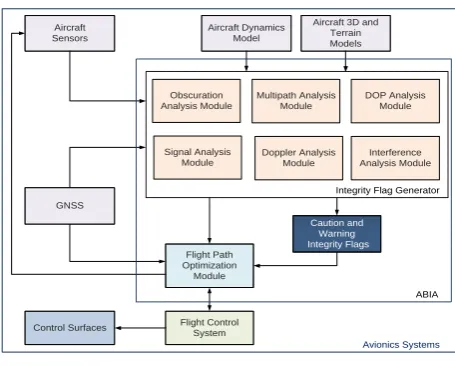
ABIA SYSTEM

During flight test activities with GNSS and Differential GNSS (DGNSS) systems [4, 5],it was observed that one or more of the following conditions was prone to cause navigation data outages or severe performance degradations: antenna obscuration, bad satellite geometries and low Carrier-to-Noise ratios (C/N0), Doppler shifts, interference and multipath. The last two problems could be mitigated by existing technology solutions (i.e., choosing a VHF/UHF data link, filtering the radio frequency signals reaching the GNSS antenna, identifying suitable locations for the GNSS antenna, etc.). However, there was little one could do in order to prevent critical events during realistic test/training manoeuvres and particular approach procedures (e.g., curved and segmented approaches) performed with high performance military A/C. The ABIA system is capable of alerting the pilot when the critical conditions for GNSS signal loss are likely to occur (within a specified maximum time-to-alert). The A/C on-board sensors provide information on the A/C relevant flight parameters (navigation data, engine settings, etc.) to an Integrity Flag Generator (IFG), which is also connected to the on-board GNSS receiver. Detailed mathematical algorithms have been developed to cope with the main causes of GNSS signal outages and degradation in flight, namely: obscuration, multipath, interference, fading due to adverse geometry and Doppler shift. Adopting these algorithms, the ABIA system is able to provide steering information to the pilot and electronic commands to the A/C flight control system, allowing real-time avoidance of safety-critical flight conditions and fast recovery of the required navigation performance in case of GNSS data losses. This is achieved by implementing both caution (predictive) and warning (reactive) integrity flags, as well as 4-Dimensional Trajectory (4DT)

optimisation models suitable for all phases of flight. Therefore, an advanced ABIA system was developed (Fig. 1). In this system, the on-board sensors provide information on the A/C relevant flight parameters (navigation data, engine settings, etc.) to an Integrity Flag Generator (IFG), which is also connected to the GNSS system. Using the available data on GNSS and the relevant flight parameters, integrity signals are generated which can be sent to the Unmanned Aircraft System (UAS) Ground Control Station (GCS) or used by a Flight Path Optimisation (FPO) module. This system addresses both the predictive and reactive nature of GNSS integrity augmentation by producing suitable integrity flags (cautions and warnings) in case of predicted/ascertained GNSS data losses or unacceptable signal degradations exceeding the Required Navigation Performance (RNP) specified for each phase of flight, and providing guidance information to the remote pilot/autopilot to avoid further data losses/degradations. To achieve this, the Integrity Flag Generator (IFG) module produces the following integrity flags [1, 2]:

 Caution Integrity Flag (CIF): a predictive annunciation that the GNSS data delivered to the avionics system is going to exceed the RNP thresholds specified for the current and planned flight operational tasks (alert status).

 Warning Integrity Flag (WIF): a reactive annunciation that the GNSS data delivered to the avionics system has exceeded the RNP thresholds specified for the current flight operational task (fault status).

ABIA

Flight Path Optimization

Module

Flight Control System Control Surfaces

GNSS

Caution and Warning Integrity Flags Aircraft

Sensors

Avionics Systems Aircraft Dynamics

Model

Aircraft 3D and Terrain Models

Multipath Analysis Module Obscuration

Analysis Module

Signal Analysis Module

Doppler Analysis Module

DOP Analysis Module

Interference Analysis Module

Integrity Flag Generator

Fig. 1. ABIA system architecture.

The following definitions of Time-to-Alert (TTA) are applicable to the ABIA system [1, 2]:

 ABIA Time-to-Caution (TTC): the minimum time allowed for the caution flag to be provided to the user before the onset of a GNSS fault resulting in an unsafe condition.

Based on the above definitions, we can define two separate models for the time responses associated to the Prediction-Avoidance (PA) and Reaction-Correction (RC) functions performed by the ABIA system (Fig. 4-2). The PA time response is given by [1]:

(1)

where:

= Time required to predict a critical condition;

= Time required to communicate the predicted failure to the FPO module; = Time required to perform the

avoidance manoeuvre.

In this case, we have . If the available

avoidance time is not sufficient to perform an adequate avoidance manoeuvre (i.e., ), the A/C will inevitably encroach on critical conditions causing GNSS data losses or unacceptable degradations. In this case, the RC time response applies:

(2)

where:

= Time required to detect a critical

condition;

= Time required to communicate the failure

to the FPO module;

= Time required to perform the correction

manoeuvre.

In general, we must have . The RC time response is substantially equivalent to what current GBAS and SBAS systems are capable of achieving. Further progress is possible adopting a suitable algorithm in the IFG module capable of initiating an early correction manoeuvre as soon as the condition

≤ TTC is violated. In this case, the direct

Prediction-Correction (PC) time response would be:

(3)

Therefore, the ABIA system can reduce the time required to recover from critical conditions if the following inequality is verified:

(4)

ABIA INTEGRITY FLAGS

The ABIA IFG module is designed to provide caution and warning flags (i.e., in accordance with the specified TTC and TTW requirements) in all relevant flight phases. The main causes of GNSS data degradation or signal losses in aviation applications were deeply analysed in [2] and are listed below:

 Antenna obscuration (i.e., obstructions from the wings, fuselage or empennage during maneuvers);

 Adverse satellite geometry, resulting in high Position Dilution of Precision (PDOP);

 Fading, resulting in reduced carrier to noise ratios (C/N0);

 Doppler shift, impacting signal tracking and acquisition/reacquisition time;

 Multipath effects, leading to a reduced C/N0 and to range/phase errors;

 Interference and jamming.

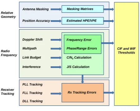
Most GNSS integrity degradations depend on the relative positions of the GNSS receiver antenna and each satellite. The relative motion of the GNSS receiver antenna and the satellites is also crucial. Therefore degradations related to one satellite do not affect the system in the same manner as the others. Specific mathematical models and associated integrity thresholds are introduced for antenna obscuration, Doppler shift, multipath, carrier, interference and satellite geometry degradations. Based on GNSS satellite observations and avionics sensor inputs, the IFG module is capable of detecting adverse conditions leading to unacceptable degradations or losses of satellite signals [1, 2]. As described in [1], A/C Position, Velocity, Time (PVT) and attitude (Euler angles) data from the on board sensors (i.e., inertial navigation systems, air data computer, etc.), GNSS data (raw measurements and PVT), and Flight Control System (FCS) actuators data are passed to the IFG module. The required navigation, flight dynamics and GNSS constellation data are extracted, together with the relevant information from an A/C Three-Dimensional Model (3DM) and from a Terrain and Objects Database (TOD). The philosophy adopted to set-up thresholds for the CIF and WIF integrity flags is depicted in Fig. 2.

CIF and WIF Thresholds Relative

Geometry

Radio Frequency

Receiver Tracking

Antenna Masking

Position Accuracy

PLL Tracking

FLL Tracking

Masking Matrixes

Estimated HPE/VPE

Rx Tracking Errors

DLL Tracking Multipath

Link Budget

Interference

C/N0Calculation

J/S Calculation Doppler Shift

Phase/Range Errors Frequency Error

Fig. 2. Integrity flag thresholds criteria.

Integrity flags are generated based on a dedicated error analysis addressing the following aspects of GNSS performance:

 Radio frequency (RF) signal errors (i.e., Doppler shift, jamming and multipath);

 Receiver Tracking Errors (RTE).

In particular, the RTE models are used to support the development of robust criteria for the RF signal thresholds, in addition to the criteria based on experimental results (e.g., ground and flight test activities with GNSS). Tables 1 and 2 list the detailed criteria adopted for each CIF and WIF threshold.

Table. 1. CIF criteria [1-3].

CIF Type Criteria

Masking

When the current A/C manoeuvre will lead to less the 4 satellite in view, the CIF shall be generated.

Satellite visibility

When one (or more) satellite(s) elevation angle (antenna frame) is less than 10 degrees, the caution integrity flag shall be generated.

DOP

When the EHE3-σ exceeds the HAL or the EVE3-σ exceeds the VAL, the CIF shall be generated.

Multipath

When the ELP exceeds 0.1 radians, the caution integrity flag shall be generated.

Tracking loops

When either

the CIF shall be generated.

C/N0

When the C/N0 is less than 26 dB-Hz the CIF shall be generated.

Jamming

When the difference between the received (incident) jammer power (dBw) and the received (incident) signal power (dBw) is 1 dB below the J/S performance of the receiver at its tracking threshold, the CIF shall be generated.

Doppler

When the C/N0 is below 28 dB-Hz and the signal is lost, the caution integrity flag shall be generated if the estimated acquisition time is less than the application-specific TTA requirements.

Table. 2. WIF criteria [1-3].

WIF Type Criteria

Masking When less than 4 satellites are in view, the WIF shall be generated.

Satellite visibility

When one (or more) satellite(s) elevation angle is less than 5 degrees, the warning integrity flag shall be generated.

DOP

When the EHE2-σ exceeds the HAL or the EVE2-σ exceeds the VAL, the CIF shall be generated.

Multipath

When the multipath ranging error shows a sudden increase with the A/C flying in proximity of the ground (below 448.5 metres), the warning integrity flag shall be generated.

When the multipath ranging error exceeds 2 metres and the A/C flies in proximity of the ground (below 500 ft AGL), the warning integrity flag shall be generated.

Tracking loops

When or

or the WIF shall be generated.

C/N0

When the C/N0 is less than 25 dB-Hz the CIF shall be generated.

Jamming

When the difference between the received (incident) jammer power (dBw) and the received (incident) signal power (dBw) is above the J/S performance of the receiver at its tracking threshold, the WIF shall be generated.

Doppler

When the C/N0 is below 28 dB-Hz and the signal is lost, the warning integrity flag shall be generated if the estimated acquisition time exceeds the application-specific TTA requirements.

FLIGHT PATH OPTIMISATION MODULE

can be solved using a variety of direct or indirect methods. All the standard components of an optimization problem are present: the A/C Dynamics Model (ADM) gives the dynamic constraints (allowing the generation of a flyable trajectory); the CIF thresholds and the current GNSS parameters define a certain number of path constraints ensuring that WIF thresholds are not exceeded on the whole trajectory; the boundary conditions include minimum, maximum, initial and final values for the various state and command variables involved in the computation (these are given by the on-board A/C sensors and by the Flight Management System (FMS), which stores the information relative to the initial flight plan). A cost function is implemented to address the minimisation of certain performance criteria. In safety-critical GNSS applications (e.g., curved/segmented precision approaches), all the necessary constraints associated to integrity degradations are included in the path constraints and the trajectory is optimised for minimum time to destination waypoint. However, more complex criteria can be set based on the actual A/C performance parameters (e.g., minimum fuel consumption) or on the characteristics of the mission (i.e., to maximise distance from another A/C, to minimise the distance from the initial waypoint, etc.).

FLIGHT DYNAMICS MODELS

As the concept of flight trajectory is deeply related to the dynamics of the body in aerial motion, flight dynamics model implementations are discussed beforehand. The focus of this research is on fixed-wing civil/military A/C; hence the Six Degree of Freedom (6DOF) and 3 Degree of Freedom (3DOF) models introduced here are specifically tailored to this category of flying platforms. Assuming the A/C to be a rigid body with a static mass distribution, a rather accurate model of its flight dynamics can be introduced, which is derived from the equilibrium of forces and momentums along the coordinate axes of a suitable Cartesian reference frame with origin in the centre of mass of the A/C (i.e., body frame). This model involves a high number of parameters to define the properties of inertia, aerodynamic stability and control forces. Adequate experimental and numerical investigations are typically required in order to define the parameters with good precision. For implementation in avionics guidance and control systems (e.g., fly-by-wire flight control systems) and for other applications including flight simulation and trajectory estimation/route planning, A/C flight dynamics are typically described by a set of Differential Algebraic Equations (DAE). The set of DAE and complementary kinematic relations defining the 6DOF rigid body dynamics of a fixed-wing A/C are [6]:

[ ̇ ̇

̇] [ ] [

] [

] (5)

[ ̇ ̇ ̇

] [

]

[

( )

( ) ( )

( )

]

(6)

[ ] [

]

[ ] [

]

(7)

[ ] [

] [ ] (8)

where:

= non-null components of the

inertia tensor [kg m2];

= components of the wind vector along the three axes of the Earth-fixed reference frame [m s-1];

= components of the aerodynamic and propulsive forces acting along the three axes of the body reference frame [N];

= components of the aerodynamic and propulsive moments acting around the three axes of the body reference frame [N m];

= components of the relative position vector between the Earth-fixed reference frame and the body centre of mass [m];

= Euler angles, respectively

representing bank, pitch and heading rotations [rad];

= translation velocity components

along the three axes of the body reference frame [m s-1];

= rotation velocity components

around the three axes of the body reference frame; respectively representing rolling, pitching and yawing rates [rad s-1];

, g = A/C weight [N] and gravity

acceleration [m s-2];

= sine and cosine operators.

associated to its rotational dynamics. The resulting 3DOF models are based on Newton’s second law expressed along the coordinate axes of the body frame and on the motion of such frame with respect to an inertial reference frame of convenience. 3DOF models can involve either a constant mass or a variable mass. Models belonging to the first category are adopted when the analysed timeframe is relatively short (so that the fuel consumption may be neglected) or when no fuel is consumed, such as in the case of sailplanes or total engine failures. The 3DOF A/C dynamics model equations can be expressed as follows [7]:

( )

(9)

( )

(10)

( )

(11)

(12)

( ) (13)

(14)

( ) (15)

where:

m = A/C mass [kg];

= longitudinal velocity [m s-1]; = thrust magnitude [N]; = angle of attack [rad]; = altitude [m];

= lift magnitude [N]; = drag magnitude [N]; = gravity acceleration [m s-2];

= flight path angle [rad]; = bank or roll angle [rad]; = heading angle [rad];

SFC = specific fuel consumption [kg/sN]; FF = fuel flow [l s-1];

= geodetic latitude [rad]; = geodetic longitude [rad];

= meridional radius of curvature [m];

= transverse radius of curvature [m].

Key assumptions adopted in the model formulation are:

 Earth’s shape is approximated as an ellipsoid using WGS-84 parameters.

 The atmosphere is considered at rest relatively to the earth.

 A standard ISA atmospheric model is adopted to describe temperature, pressure and density variations as a function of altitude.

 The A/C is modelled as a rigid body with a vertical plane of symmetry.

 The A/C mass reduction in flight is due to fuel consumption only.

 Thrust, aerodynamic forces and weight act on the A/C Centre of Gravity (CG).

 All manoeuvres are well coordinated and no sideslip is present.

 The flight is subsonic and the thrust vector is aligned with the longitudinal axis of the A/C (body frame).

The classical formulas for lift and drag are:

S (16)

(17)

where is the lift coefficient, is the drag coefficient, is the wing area and is the air density. Both and

can be obtained from the A/C polar curves when available (practical avionics implementations typically adopt lookup tables). Alternatively, the lift and drag coefficients are computed using the available derivatives. For the lift coefficient, the following equation is used:

(18)

where is the zero-alpha lift (i.e., the lift coefficient at zero angle of attack), and is the alpha derivative (i.e., the first-order variation of with respect to the angle of attack). For the drag coefficient a similar approach can be adopted and the following equation is used:

( )

(19)

where is the minimum drag coefficient of the airplane, is the lift at minimum drag, which is usually but not necessarily equal to , is the wing span and is the Oswald efficiency factor (for conventional fixed-wing A/C with moderate aspect ratio and sweep, is typically between 0.7 and 0.85).

TRAJECTORY OPTIMISATION ALGORITHMS

As discussed, the IFG outputs (CIFs and WIFs) are used in the FPO module. The key requirement of the FPO module is to generate guidance information that optimize the short-term Autopilot and Flight Director System (A&FDS) control parameters (e.g., attitude angles and airspeed), as well as the medium/long-term trajectory to be flown. The information update process starts from the current information stored in the Flight Management System (FMS) and produces a new set of geometric/dynamic constraints in all conditions where CIFs are raised (to avoid WIFs). A trajectory optimisation process is then initiated to meet the specified mission objectives and to comply with this new set of constraints. The results obtained from the computation of the optimal trajectory can be utilized as new inputs to the IFG software (both in real-time and mission-planning implementations), so further updates can be performed when needed to prevent the triggering of CIFs and WIFs. From a practical point of view, trajectory optimisation can be defined as the action of finding the inputs to a given system characterised by a set of equations of motion and dynamic constraints, which will maximise or minimise specific parameters (e.g., time, fuel consumption, distance from another A/C, relative velocities). In most cases, optimisation problems cannot be solved analytically and, therefore, numerical iterative methods need to be used. One of the key challenges of the online trajectory optimisation task is to produce results in real-time (real-time here is intended for the specific application/scenario involved), since the mathematical algorithms and the associated numerical solvers have to be capable of producing accurate and usable outputs in a relatively short time. Offline and online A/C trajectory optimisation tasks are typically formulated as Optimal Control Problems (OCP). This is because optimal control theory provides a well-established framework for the determination of dynamic systems optimal trajectories (in a mathematical sense). In the OCP formulation, the trajectory optimisation problem can be analytically stated as follows [9, 10]:

“Determine the states ( ) , the controls ( ) , the parameters , the initial time and the final time , that optimise the performance index:

[ ( ) ( ) ] ∫ [ ( ) ( ) ] (20)

subject to the dynamic constraints:

̇( ) [ ( ) ( ) ] (21)

to the path constraints:

[ ( ) ( ) ] (22)

and to the boundary conditions:

[ ( ) ( ) ( ) ( ) ] (23)

where is the Mayer term and is the Lagrange term of the cost function expressed in a Bolza form.”

objectives and constraints. Those can be derived from Air Traffic Management (ATM) imposed requirements, flight plan/mission objectives, Separation Maintenance and Collision Avoidance (SM/CA), and environmental requirements. Thus, the optimisation process needs to find the best trade-off between all objectives subject to the dynamics/operational constraints associated with the platform, the planned mission and the current flight profile/phase. Clearly, different sets of data (from widely differing sources) and significantly different objectives/constraints can be used at the mission planning stage and in real-time flight trajectory optimisation tasks. ABIA offers the advantage of meeting the requirements of strategic and tactical air operation tasks, with a possibility to also enhance the performance of SM/CA systems that rely on GNSS as the primary source of navigation data. These include modern cooperative SM/CA systems (e.g., ADS-B) or non-cooperative sensors integrated with GNSS-driven Guidance, Navigation and Control (GNC) systems. For a practical implementation, some additional considerations have to be made. The new trajectory determined by the FPO module has to be completely flyable by the A/C and the mission (defined in the FMS flight plan) shall not be compromised by the new trajectory. Additionally, the new trajectory shall not lead to other hazards like terrain, traffic or weather. As a consequence, the FPO module has to be designed to allow the dynamic setting of boundary conditions for the entire set of variables involved. From the discussion above the following key requirements are derived:

The FPO module shall react to any CIF/WIF triggering as follows:

 Initiating an early-correction loop that prevents the occurrence of a WIF, as soon as CIF is generated.

 Initiating an immediate (emergency) correction in the unlikely event of a WIF not preceded by a CIF.

As soon as activated, the FPO module shall set dynamic constraints that allow the computation of an optimal flight trajectory that prevents the triggering of new CIFs/WIFs and that minimises the deviations from the original A/C trajectory (e.g., FMS flight plan).

CONSTRAINTS AND BOUNDARY CONDITIONS

Most GNSS integrity degradations depend on the relative positions of the GNSS receiver antenna and each satellite. The relative motion of the GNSS receiver antenna and the satellite is also crucial. Therefore degradations related to one satellite do not affect the system in the same manner as the others. An analysis of the different type of degradations results in inferring that a common criterion based on satellite elevation variation in the body frame can be adopted as a geometric constrain in the trajectory optimisation process. This applies to all degradations except Doppler shift (so, for this phenomenon a separate analysis is required). The elevation and azimuth angles in body frame (blue) are depicted in Fig. 3 where is the satellite position, is the satellite position in XY

frame, is the line of sight vector, is the elevation angle and is the azimuth angle. The right-hand rule gives the direction of rotation of both elevation and azimuth angles. Considering the top view of the A/C, when the elevation angle increases in the positive direction (going up), the azimuth is rotating in a clockwise direction. The elevation angle in the body frame is computed using the simple trigonometry relation:

₍

) (24)

where is the Z-axis component of the line of sight vector. In order to be used as a dynamic constraint for trajectory optimisation, the elevation angle to each satellite is associated to Euler angles by converting the Line-of-Sight (LOS) vector from the East-North-Up (ENU) reference frame to the body frame. The positions of the A/C and satellite are given in the ENU frame, so the LOS vector is computed using:

⃗ ⃗⃗⃗ ⃗⃗⃗⃗ (25)

where is the receiver position vector in the ENU frame.

X

Y Ps

Z

R

Az E

Psxy

Fig. 3. Elevation and azimuth in body frame.

The conversion in body frame is obtained using the matrix:

D [

] (26)

where:

= sine of the pitch angle;

= cosine of the pitch angle;

= sine of the bank angle; = cosine of the bank angle;

= sine of the yaw angle;

= cosine of the yaw angle.

The magnitude of the Doppler shift produce in the signal received from to the nth satellite is a function of the relative velocity measured along the satellite-A/C LOS. The magnitude of the Doppler shift can be calculated by:

T

χn’ En

χn

0°

N

90°

180°

270°

S

E W

’ 0°

180°

225°

270° 45° 90°

135°

315°

where:

⃗⃗⃗⃗ = nth satellite velocity component along the LOS;

⃗⃗⃗⃗ = A/C velocity projection along the LOS; c = speed of light [m s-1];

f = GNSS signal frequency [Hz];

= angle between the A/C velocity vector and the nth satellite LOS.

When the Doppler CIF thresholds are exceeded, the FPO module initiate an optimisation process aiming to avoid any further observed increase in Doppler shift. In particular, the implemented algorithm studies the variations of ⃗⃗⃗⃗ and ⃗⃗⃗ for each tracked satellite and imposes geometric constraints to the trajectory that are accounted for in the trajectory optimisation process. With reference to the geometry illustrated in Fig. 3, the following trigonometric relationship holds true:

( ) = (28)

where:

= A/C velocity vector;

= elevation angle of the nth satellite;

= relative bearing of the A/C to the satellite;

= azimuth of the LOS projection in the antenna plane.

Reductions of elevation angles lead to increases in Doppler shift, while drives increments or decrements in Doppler shift depending on the size of the angle and the direction of the A/C velocity vector. From Eq. (27) and Eq. (28), we can determine the A/C-satellite relative geometric conditions that maximise or minimise Doppler shift. In particular, combining the two equations we obtain:

( ⃗⃗⃗⃗⃗ ⃗⃗⃗⃗⃗ ) (29)

Eq. (29) shows that both the elevation angle of the satellite and the A/C relative bearing to the satellite affect the magnitude of the Doppler shift. In particular, reductions of lead to increases in Doppler shift, while drives increments or decrements in Doppler shift depending on the size of the angle and the direction of the A/C velocity vector.

Fig. 4. Reference geometry for Doppler shift analysis. By inspecting Fig. 4, it is evident that a relative bearing of 90° and 270° would lead to a null Doppler shift as in this case there is no component of the A/C velocity vector

( ⃗⃗⃗⃗ in this case) in the LOS to the satellite. However, in all other cases (i.e., ⃗⃗⃗⃗ ), such a component would be present and this would lead to increments or decrements in Doppler shift depending on the relative directions of the vectors and ⃗⃗⃗⃗ . This fact is better shown in Fig. 5, where we assume steady flight without loss of generality.

Fig. 5. Reference geometry for Doppler shift manoeuvre corrections. As the time required for typical A/C heading change manoeuvres is much shorter than the timeframe associate to significant satellite constellation changes, each satellite can be considered stationary in the body reference frame of the manoeuvring aircraft. Therefore, during manoeuvres leading to Doppler CIFs, we can consider an initial aircraft velocity vector ⃗⃗⃗ and define path constraints that avoid the Doppler WIF. This can be done by imposing that the aircraft increases the heading rates towards the directions ⃗⃗⃗ or -⃗⃗⃗ and minimises the heading rates towards the directions ⃗⃗⃗⃗⃗ and - ⃗⃗⃗⃗⃗ . The choice of ⃗⃗⃗ or -⃗⃗⃗ is based simply on the minimum required heading change (i.e., minimum required time to accomplish the correction). Regarding the elevation angle (E) dependency of Doppler shift, Eq. (29) shows that minimising the elevation angle becomes an objective also in terms of Doppler trajectory optimisation.

COST FUNCTIONS

The selection of the optimal trajectory is based on minimising a cost function of the form [11]:

∫[ ( )] (30)

where [ ] is the specific fuel consumption,

( ) is the thrust profile and { } are the weightings attributed to time and fuel minimisation objectives. In safety-critical UAS applications, this cost function can be expanded to include other parameters such as the distance of the host A/C from the avoidance volume associated with a ground obstacle or a conflicting air traffic [12]:

∫[ ( )]

∫ ( )

(31)

associated with the obstacle, [ ( )] is the estimated minimum distance of the avoidance trajectory from the avoidance volume, is the time at which the safe avoidance condition is successfully attained and { } are the weightings attributed to time, fuel, distance and integral distance respectively. In time-critical avoidance tasks appropriate higher weightings are used for time and distance cost elements and an automated gain control function can be implemented taking into account the host A/C-obstacle relative dynamics.

MISSION PLANNING OPTIMISATION

Based on the literature review [9-11], the Radau pseudospectral method was selected for the ABIA mission planning implementation (offline IFG and FPO modules). This widely used methods employ orthogonal collocation Gaussian quadrature implicit integration, where collocation is performed at the Legendre-Gauss-Radau points. The Generalised Pseudospectral Optimal Control Software, version 2 (GPOPS-II) was chosen for ABIA due to its availability in the public domain and its documented suitability for aerospace applications. GPOPS-II is implemented as a MATLAB toolbox were the user defines the dynamics/path constraints, the boundary conditions and the cost functions that apply to a specific OCP. The user can also define a number of parameters used in the optimisation process, including the quadrature mesh characteristics, the maximum number of iterations and the numerical differentiation method. Further details about GPOPS-II and some examples of aerospace OCPs can be found in (Patterson et al., 2014). The suitability of these techniques for ATM and Air Traffic Flow Management (ATFM) strategic and tactical operations has been demonstrated in recent research [13].

REAL-TIME OPTIMISATION

For real-time FPO module implementations, a Direct Constrained Optimisation (DCO) method is implemented. In this method the aircraft dynamics model is used to generate a number of feasible flight trajectories that also satisfy the GNSS constraints. The feasible trajectories are calculated by initialising the aircraft dynamics model with a Manoeuvre Identification Algorithm (MIA). The MIA allows identifying a sub-set of ADM equations (and the associated boundary conditions of states and controls) that must be integrated to predict future states and to determine the optimal controls that minimise the cost functions. A schematic representation of the FPG module DCO implementation is shown in Fig. 6. Although this method does not implement an iterative algorithm that converges to the mathematical optimum, it is preferred for real-time safety-critical applications due to its robustness, much reduced complexity and faster convergence rate. Additionally, the DCO prevents problems of non-convergence or divergence frequently experienced in OCPs for highly non-linear dynamic systems. In the ABIA FPG implementation, the DCO algorithm is designed so that the deviations from the pre-planned flight

trajectory (e.g., FMS flight plan) are minimised. This is achieved by introducing additional geometric (path) constraints in the process and implementing a Bézier approximation curve algorithm to guarantee smoothness of the resulting aircraft trajectory [14].

Manoeuvre Identification

GNSS Constraints

Boundary Conditions Cost Functions

DCO Numerical Solver

Aircraft Systems Data

- Landing gear - Navigation - Propulsion - Autopilot - Flight Controls

Flight Management System

- Flight Plan - Weather Data - A/C Performance Data - Navigation Database

ABIA IFG Module Output

- Caution Flags - Warning Flags

GNSS Constellation

- Satellite Position - Satellite Azimuth - Satellite Elevation

Dynamic and Path Constraints

Fig. 6. DCO implementation scheme.

OPTIMISATION CRITERIA

In both real-time and mission-planning implementations, the flight trajectory optimisation algorithm is initiated when integrity degradations are predicted (CIF generated) by the IFG module. The optimisation criteria adopted in the FPG module are the following:

 With 5 satellites in view, the value of En for each satellite tracked shall be 5 degrees greater than the threshold value causing the activation of any CIF.

 With 4 satellites in view, the value of En for each satellite tracked shall be 10 degrees greater than the threshold value causing the activation of any CIF.

 If the CIF is not due to Doppler shift, the minimum elevation limit is set to 5 degrees above the current SV elevation angle.

 If the CIF is due to Doppler shift, the aircraft heading rates are increased towards the directions ⃗⃗⃗ or -⃗⃗⃗ and reduced in the directions ⃗⃗⃗⃗⃗ and - ⃗⃗⃗⃗⃗ . The choice of

⃗⃗⃗ or - ⃗⃗⃗ is based on the minimum required heading change.

 Constrained Geometric Optimisation (CGO) or Pseudospectral Multi-Objective (PMO) Trajectory Optimisation Techniques are used for real-time FPG implementations and for offline mission-planning applications respectively.

The boundary values of each parameter involved in the trajectory optimisation process are obtained from the following sources:

 Planned Flight Trajectory (PFT), which define the final condition of the optimization problem. The final condition gives the point when the A/C will go back on the initially planned trajectory (e.g., the trajectory stored in the FMS).

 A/C Dynamic Constraints (ADC), which define the minimum and maximum values of the state and control variables.

 Satellite Constellation Data (SCD), which provide the azimuth and elevation boundaries for the path constraints.

SBAS/GBAS INTEGRITY FLAG GENERATION

The ABIA models can be used to enhance the performance of existing SBAS and GBAS systems. In the proposed implementation, Vertical and Lateral Protection Level (VPL and LPL) for SBAS and GBAS are calculated in line with the performance standards for WAAS and LAAS [15-18]. These are compared to the Vertical and Lateral Alert Limits (VAL and LAL) specified for each flight phase (for SBAS) and for each GNSS Landing System (GLS) class (for GBAS). The criteria for producing SBAS/GBAS CIFs and WIFs are listed below:

 When VPLSBAS exceeds VAL or HPLSBAS exceeds HAL, the WIF is be generated.

 When PVPLGBAS exceeds VAL or PLPLGBAS exceeds LAL, the CIF is generated.

 When VPLGBAS exceeds VAL or HPLGBAS exceeds HAL, the WIF is generated.

As both SBAS and GBAS use redundant GNSS satellite observations to support Fault Detection and Exclusion (FDE) within the GNSS receiver, some additional integrity flag criteria can be introduced. Based on FAA technical standard orders TSO-C145C and TSO-C146C [19], a current generation WAAS-enabled GNSS receiver uses RAIM for instances when the augmentation signal becomes unavailable. In this WAAS/RAIM integration scheme, the minimum number of satellites required for FDE is 6. At present, no information is available regarding the provision of RAIM features within LAAS-enabled GNSS receivers. Therefore, we can assume the inclusion of a basic form of RAIM within such receiver (i.e., at least 5 satellites are required for FDE). Based on these assumptions, the number of satellites in view can be used to set additional integrity thresholds for SBAS and GBAS:

 When the number of satellites in view is less than 6, the GBAS CIF is generated.

 When the number of satellites in view is less than 5, the GBAS WIF is generated.

 When the number of satellites in view is less than 7, the SBAS CIF is generated.

 When the number of satellites in view is less than 6, the SBAS WIF is generated.

These new thresholds are well suited for implementation into the ABIA IFG.

SIMULATION CASE STUDIES

In order to validate the design of the ABIA IFG module and the synergies with GBAS and SBAS, some detailed simulation case-studies were performed on AEROSONDE “Laima” UAS platform. All simulated A/C trajectories included the following flight phases and flight legs:

 Takeoff: Straight Climb (SC) leg;  Route Capture: Turning Climb (TC) leg;

 Cruise Phase: Straigh and Level (SL) and/or Level Turn (LT) legs;

 Initial Descent: Turning Descent (TD) and/or Straight Descent (SD) leg;

 Final Descent: Straight descent leg to Approach (AP).

The duration of each flight leg was defined in accordance with the typical mission profiles of the designated aircraft types. The terrain profile was assumed to be flat and free from man-made features. No jamming sources were considered in the simulation case studies. For the avionics GPS receiver characteristics, we used a C/A code receiver with a flat random vibration power curve from 20Hz to 2000Hz with amplitude of 0.005 and the oscillator vibration sensitivity ( ) parts/g. Additionally, a third-order loop noise bandwidth of 18 Hz was considered and a maximum LOS jerk dynamic stress of 10g/s=98 was assumed. Finally, the following simplified antenna gain pattern was adopted:

( ) (32)

This resulting antenna gain pattern is shown in Fig. 7.

17-Feb-2012 39

© Roberto Sabatini, 2012 39

Antenna Gain (dB)

Elevation

Fig. 7. Simplified GPS antenna gain pattern.

geometric accuracy degradations, S/N, multipath and Doppler shift were generated. The relevant AEROSONDE geometric parameters were extracted from the literature to draw a detailed 3-D model of the aircraft (Holland et al., 2001), (Burston et al., 2014), (Aircraft Drawings, 2012). The AEROSONDE 3-D CATIA model obtained is shown in Fig. 8.

Fig. 8. AEROSONDE 3-D CATIA model.

The aircraft has a wing span of 2.9 m, a length of 2.2 m, a wing area of 0.55 m² and a Propeller Radius of 0.25 m. The AEROSONDE version considered is equipped with a 24cc fuel injected premium unleaded gasoline engine and its overall weight is 13 -15 kg (29-33 lbs.) depending on payload, fuel tank and battery configurations. The payload is up to 2 kg (4.4 lbs.) with full fuel load (5 kg). The UAV can reach a speed of 80-150 km/hr (50-93 miles/hour) in cruise and 9 km/hour (6 miles/hr) in climb. The operational range is greater than 3,000 km with an endurance of 30 hours at 0.1 – 6 km altitude (depending on payload). Communication tasks are accomplished by V/UHF radio and/or LEO satellites. The location of the AEROSONDE GPS antenna is shown in Fig. 9.

Fig. 9. AEROSONDE UAV antenna location. Adapted from[20]. To speed-up and automate the process of Antenna Masking Matrix (AMM) generation, an Automatic Masking Profile Computation (AMPC) software was developed (Fig. 10).

Fig. 10. AMPC logic diagram.

The AMPC software populates a database (look up tables) containing the obscuration information of GNSS satellite signals for different aircraft roll and pitch angles. This is accomplished by implementing two different modules in the AMPC: the first is used to transform the aircrafts CAD model in a mesh of small triangular surfaces that allows straightforward computations of line/surface intersections in a MATLABTM environment; the second is used to rotate the aircraft in pitch and roll (bank), and to calculate the intersections between the aircraft structure (i.e., fuselage, wings and tail) and the line-of-sight (LOS) to all satellites in view as illustrated in Fig. 8. After creating the 3-D aircraft surface model, the corresponding CAD file was transformed in a Stereolithography (STL) file format. An STL file is a convenient representation of a complex 3D surface geometry, made by a number of oriented triangles (mesh). Each of these triangles is described by two elements: the first is a unit normal vector to the facet; the second element is a set of three points (listed in counter clockwise order) representing the vertices of the triangle. This representation is ideally suited for the ABIA simulation environment. As an example, the AEROSONDE mesh imported and plotted in MATLABTM is illustrated in Fig. 11.

Fig. 11. AEROSONDE mesh in MATLABTM_.

STL File Import

MATLAB Mesh File

Roll Matrix Application

Ray Definition

Intersection Function Application

Pitch Matrix Application

Ray Definition

Intersection Function Application 3-D CAD

Model

−1500

−1000

−500 0 500 1000 1500

−

1500

−

1000

−500 0

500 1000

−400

−200 0 200 400 600

−1500

−1000

−500 0 500 1000 1500

−1500

−1000

−500 0

500

1000

−400

−200 0 200 400 600

-Using this representation, the AMM is generated calculating all possible intersections of the aircraft body (all triangular surfaces) with the LOS antenna-satellites during pitch and roll motion (Fig. 12).

Fig. 12. AEROSONDE masking profile simulation. The simulated AEROSONDE UAV trajectory, generated using the aircraft 6DOF model [21, 22], is shown in Fig. 13. It includes the seven flight legs described above (SC = 450 s, TC = 450 s, SL = 1300 s, LT = 450 s, TD = 450 s, SD = 200 s and AP = 100 s), for a total of 3400 s.

Fig. 13. AEROSONDE UAV simulated trajectory.

The results of the AEROSONDE IFG simulation are listed in Table 3. The CIFs were always triggered at least 2 seconds before the successive WIFs. All CIFs were followed by WIFs leading to DRCIF of 100%.

Additionally, all CIFs were followed by a WIF, A total of 13 CIFs were generated and 3 were not associated to WIFs. Therefore, the False Alarm Rate (FAR) was FARCIF=23%. These results corroborate the general

validity of the models developed for the CIF/WIF thresholds.

Table 3. Integrity Flags for AEROSONDE.

LEG CIF Time WIF Time

LT

2241 ~ 2311 s, 2413 ~ 2485 s, 2491 ~ 2650 s

2259 ~ 2263 s, 2273 ~ 2283 s, 2432 ~ 2436 s, 2446 ~ 2485 s, 2609 ~ 2612 s, 2621 ~ 2630 s

TD

2688 ~ 2752 s, 2811 ~ 2881 s, 2944 ~ 3012 s, 3079 ~ 3100 s

2690 ~ 2739 s, 2814 ~ 2869 s, 2946 ~ 3003 s, 3081 ~ 3100 s

SD --- ---

AP 3301 ~ 3400 s 3303 ~ 3400 s

Fig. 14 shows the AEROSONDE UAV flight trajectory and illustrates the portion of the TMA where GBAS is available. In this case, GBAS provides information when the AEROSONDE is flying the legs number 5 (TD), 6 (SD) and 7 (AP). The aircraft enters the GLS Coverage Area (GCA) during the TD leg after 2745 seconds from take-off and 205 seconds before landing (end of the simulation). Use of SBAS/GBAS approach modes is assumed in legs 6 (SD) and 7 (FA).

Fig. 14. AEROSONDE UAV simulated trajectory.

The following assumptions are adopted for the SBAS/GBAS simulation and the associated parameters are set in line with the applicable standards [15-18]:

 The SBAS equipment is class 3 and is used for Lateral/Vertical Navigation (LNAV/VNAV) and Localizer Performance with Vertical Guidance (LPV 1/LPV2) operations.

 The Airframe Multipath Designator (AMD) is type A.  The number of GBAS reference receivers is 4.  The GBAS service coverage is 20 NM from the

Landing Threshold Point (LTP).

−1000 0 1000 2000 3000

−2000 −1000 0 1000 2000 −500

0 500 1000 1500 2000 2500

- GSL class is F, the Airborne Accuracy Designator (AAD) is B, and the Ground Accuracy Designator (GAD) is B.

The SBAS WIFs and CIFs recorded during the flight are listed in Table 4.

Table 4. CIF and WIF for SBAS (AEROSONDE).

LEG CIF WIF

LT 2201 ~ 2650 s 2445 ~ 2448 s, 2296 ~ 2358 s,

2453 ~ 2650 s

TD 2651 ~ 3100 s 2832 ~ 2869 s, 2701 ~ 2739 s,

3081 ~ 3093 s

AP

L/VNAV --- ---

LPV 1 --- 3161 ~ 3400 s

LPV 2 --- 3161 ~ 3400 s

The GBAS integrity flags generated during the final portions of the flight are listed in Table 5.

Table 5. CIF and WIF for GBAS (AEROSONDE).

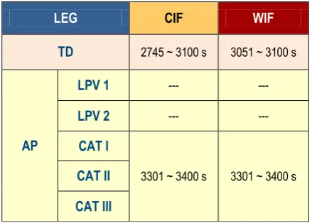
LEG CIF WIF

TD 2745 ~ 3100 s 3051 ~ 3100 s

AP

LPV 1 --- ---

LPV 2 --- ---

CAT I

3301 ~ 3400 s 3301 ~ 3400 s

CAT II

CAT III

Table 6 lists all CIFs and WIFs generated by SBAS, GBAS and ABIA in the various flight phases.

Based on these simulation case studies, it is evident that the ABIA system works synergically with SBAS and GBAS, enhancing integrity levels in the various flight phases. The ABIA algorithms are capable of generating suitable predictive and reactive flags (CIFs and WIFs) in the same flight phases where SBAS and GBAS are designed to operate but using different principles (i.e., differing input data and integrity models/thresholds). Therefore, the integration of ABIA with SBAS and GBAS is an opportunity for future research towards the development of a Space-Ground-Avionics Augmentation Network (SGAAN) suitable for manned and unmanned aircraft applications and for a variety of mission-critical and safety-critical aviation applications, including flight test, precision approach and automatic landing.

Table.6. CIF and WIF for ABIA, SBAS and GBAS.

LEG CIF WIF

LT

ABIA

2241 ~ 2311 s, 2413 ~ 2485 s, 3491 ~ 2650 s

ABIA

2259 ~ 2263 s, 2273 ~ 2283 s, 2432 ~ 2436 s, 2446 ~ 2485 s, 2609 ~ 2612 s, 2621 ~ 2630 s

SBAS

2201 ~ 2650 s 2201 ~ 2650 s SBAS

TD

ABIA

2688 ~ 2752 s, 2811 ~ 2881 s, 2944 ~ 3012 s, 3079 ~ 3100 s

ABIA

2690 ~ 2739 s, 2814 ~ 2869 s, 2946 ~ 3003 s, 3081 ~ 3100 s

SBAS

2651 ~ 3100 s 2651 ~ 3100 s SBAS

GBAS

2745 ~ 3100 s 3051 ~ 3100 s GBAS

AP

L/VNAV

ABIA

3301 ~ 3400 s

ABIA

3303 ~ 3400 s

LPV 1 _SBAS

3161 ~ 3400 s

LPV 2

CAT I ABIA

3301 ~ 3400 s

GBAS

3301 ~ 3400 s

ABIA

3303 ~ 3400 s

GBAS

3301 ~ 3400 s

CAT II

CAT III

To test the FPG module ability to optimise the aircraft flight trajectories in mission-planning and real-time ABIA implementations, a flight segment was extracted from leg 5 (CIFs/WIFs are illustrated in Fig. 15) and used to test the PMO and CGO flight path optimisation techniques. The selected flight segment is shown in Fig. 16.

Fig. 16. TD leg segment with CIF and WIF.

Fig. 17 shows the results obtained implementing the PMO technique with a 3DOF dynamic model. In this case, the trajectory optimisation loop took 8.12 seconds to complete in a standard PC equipped with an Intel i7 quad-core processor and 8 GB RAM.

Fig. 17. TD leg segment optimised with PMO.

The trajectory obtained with the CGO technique is shown in Fig. 18. In this case, the trajectory optimisation loop took 0.42 seconds to complete in a standard PC equipped with an Intel i7 quad-core processor and 8 GB RAM.

Fig. 18. TD leg segment optimised with CGO.

Further AEROSONDE simulations showed that, based on flight path length and aircraft dynamics (initial conditions), the time required for flight path optimisation varied between 5 and 220 seconds for the PMO and

between 0.3 and 0.9 seconds for the CGO. Based on these results, it is evident that the PMO algorithms cannot be directly employed in real-time ABIA applications. This is because, even with the relatively benign flight dynamics of a small UAV like the AEROSONDE, the time required to perform trajectory optimisation is too long for real-time path following tasks in Automatic Flight Control System (AFCS). As already mentioned, the PMO technique is capable of generating a mathematical optimum and is better suited for ABIA mission-planning/ATM applications (i.e., ground-based and avionics mission planning tools). It is therefore concluded that the adoption of PMO/CGO techniques in the ABIA FPG module would allow an efficient exploitation of the IFG module predictive features both in mission planning and real-time trajectory optimisation problems, potentially meeting GNSS integrity requirements for ATM online operations and AFCS/ABIA integration for GLS down to CAT II/III.

CONCLUSIONS AND FUTURE WORK

performed, it is concluded that the ABIA system works synergically with SBAS and GBAS, enhancing integrity levels in all flight phases, from initial climb to final approach. The ABIA algorithms are capable of generating suitable predictive and reactive flags (CIFs and WIFs) in the same flight phases where SBAS and GBAS are designed to operate. Therefore, the integration of ABIA with SBAS/GBAS is a clear opportunity for future research towards the development of a Space-Ground-Avionics Augmentation Network (SGAAN) suitable for manned and unmanned aircraft applications and for a variety of mission-critical and safety-critical aviation applications, including UAS Sense-and-Avoid (SAA), precision approach and automatic landing. Further research is focusing on the following areas:

 Study the potential applications of ABIA to cooperative and non-cooperative UAS SAA [23].

 Extend the ABAS/ABIA concept to other Communication, Navigation and Surveillance/Air Traffic Management (CNS/ATM) systems for Performance Based Operations (PBO) and 4D trajectory management [24-26].

 Investigate the potential of ABAS/ABIA techniques to enhance GNSS integrity in aircraft surface operations [27].

 Investigate the potential of ABAS/ABIA concepts to support aviation forensic applications (i.e., accident and incident investigation).

 Assess the potential synergies between ABIA and RAIM techniques, including enhanced RAIM (eRAIM) and predictive RAIM (pRAIM) in a multi-constellation GNSS environment.

REFERENCES

[1] R. Sabatini, T. Moore, and C. Hill, “A New Avionics Based GNSS Integrity Augmentation System: Part 1 – Fundamentals,” Journal of Navigation, vol. 66, no. 3, pp. 363-383, May 2013. DOI: 10.1017/S03734633 13000027

[2] R. Sabatini, T. Moore, and C. Hill, “A New Avionics Based GNSS Integrity Augmentation System: Part 2 – Integrity Flags,” Journal of Navigation, vol. 66, no. 4, pp. 511-522, June 2013. DOI: 10.1017/S03734633 13000143

[3] R. Sabatini, T. Moore, C. Hill and S. Ramasamy, “Investigation of GNSS Integrity Augmentation Synergies with Unmanned Aircraft Sense-and-Avoid Systems”, SAE Technical Paper 2015-01-2456, SAE 2015 AeroTech Congress & Exhibition, Seattle, Washington, USA, 2015. DOI: 10.4271/2015-01-2456

[4] R. Sabatini and G. Palmerini, “Differential Global Positioning System (DGPS) for Flight Testing,” NATO Research and Technology Organization

(RTO) – Systems Concepts and Integration Panel (SCI), AGARDograph Series RTO-AG-160, Vol. 21, Oct 2008. URL: www.dtic.mil/get-tr-doc/pdf?AD= ADA 493532

[5] R. Sabatini, T. Moore and C. Hill, “Avionics-Based GNSS Integrity Augmentation for Unmanned Aerial Systems Sense-and-Avoid,” Proceedings of 27th International Technical Meeting of the Satellite Division of the Institute of Navigation: ION GNSS+ 2014, Tampa, Florida, USA, 2014.

[6] W. F. Phillips, “Mechanics of Flight“ John Wiley & Sons, 2004.

[7] A. Valenzuela, and D. Rivas, “Conflict Resolution in Converging Air Traffic Using Trajectory Patterns”, Journal of Guidance, Control, and Dynamics, Vol. 34, no. 4, 2011, pp. 1172-1189.

[8] Rao, A.V. (2010-b), “Trajectory Optimization”, In Encyclopedia of Aerospace Engineering, John Wiley & Sons Ltd.

[9] M. P. Hansen, “Tabu Search Multiobjective Optimisation: MOTS”, in proceedings of 13th International Conference on Multiple Criteria Decision Making (MCDM '97), Cape Town, South Africa, 1996

[10] J. A. Lennon and E. M. Atkins, “Preference-Based Trajectory Generation”, in proceedings of AIAA Infotech@Aerospace 2007 (I@A 2007), Rohnert Park, CA, USA, 2007. DOI: 10.2514/6.2007-2973

[11] A. V. Rao, “Survey of Numerical Methods for Optimal Control”, Advances in the Astronautical Sciences, vol. 135, pp. 497-528, 2010

[12] S. Ramasamy, R. Sabatini and A. Gardi, “LIDAR Obstacle Warning and Avoidance System for Unmanned Aerial Vehicle Sense-and-Avoid”, Aerospace Science and Technology, vol. 55, 2016.

[13] Gardi, A., Sabatini, R., Ramasamy, S. (2016), “Multi-Objecive Four Dimesional Trajectory Optimisation in the ATM Context”, Progress in the Aerospace Sciences, April 2016. DOI: 10.1016/j.paerosci.2015.11.006

[14] Delahaye, D., Puechmorel, S., Tsiotras, P., and Feron, E., “Mathematical Models for Aircraft Trajectory Design: A Survey”, Lecture Notes in Electrical Engineering, Vol. 290, Air Traffic management and Systems, pp. 205-247, 2014

[15] RTCA, DO-229D - Minimum Operational Performance Standards for Global Positioning System/Wide Area Augmentation System Airborne Equipment, Washington DC, USA, 2006.

[17] RTCA DO-253C - Minimum Operational Performance Standards for GPS/GBAS Airborne Equipment, Radio Technical Commission for Aeronautics, Special Committee No. 159. Washington DC (USA), December 2008.

[18] RTCA DO-246D - GNSS-Based Precision Approach Local Area Augmentation System (LAAS) Signal-in-Space Interface Control Document (ICD), Washington DC, USA, 2008.

[19] FAA, Global Positioning System Wide Area Augmentation System (WAAS) Performance Standard, Washington DC (USA), 2008.

[20] J. Maslanik, Seminar on AEROSONDE UAV, Colorado Center for Astrodynamics Research (CCAR), University of Colorado at Boulder, 2002. Available online at: http://www2.hawaii.edu/ ~jmaurer/uav/#specifications

[21] Unmanned Dynamics (2003). “Aerosim Blockset User’s Guide.” Version 1.01. Unmanned Dynamics LLC, Hood River, OR (USA). Document available online at: https://people.rit.edu/pnveme/EMEM682n/ Matlab_682/aerosim_ug.pdf (accessed 3rd June 2012).

[22] M. T. Burston, R. Sabatini, R. Clothier, A. Gardi and S. Ramasamy, “Reverse Engineering of a Fixed Wing Unmanned Aircraft 6-DoF Model for Navigation and Guidance Applications.” Applied Mechanics and Materials, Vol. 629, pp. 164-169, October 2014. DOI: 10.4028/www.scientific.net /AMM.629.164

[23] S. Ramasamy, R. Sabatini and A. Gardi, “Towards a Unified Approach to Cooperative and Non-Cooperative RPAS Detect-and- Avoid”, Fourth Australasian Unmanned Systems Conference 2014 (ACUS 2014), Melbourne, Australia, 2014. DOI: 10.13140/2.1.4841.3764A.

[24] Gardi, R. Sabatini, T. Kistan, Y. Lim, and S.

Ramasamy, “4-Dimensional Trajectory

Functionalities for Air Traffic Management Systems”, in proceedings of Integrated Communication, Navigation and Surveillance Conference (ICNS 2015), Herndon, VA, USA, 2015. DOI: 10.1109/ICNSURV.2015.7121246

[25] S. Ramasamy, R. Sabatini and A. Gardi, “Novel Flight Management Systems for Improved Safety and Sustainability in the CNS+A Context”, Proceedings of Integrated Communication, Navigation and Surveillance Conference (ICNS 2015), Herndon, VA, USA, 2015. DOI: 10.1109/ICNSURV.2015.7121225

[26] S. Ramasamy and R. Sabatini, “A Unified Approach to Cooperative and Non-Cooperative Sense-and-Avoid”, Proceedings of International Conference on Unmanned Aircraft Systems (ICUAS

2015), Denver, CO, USA, 2015. DOI:

10.1109/ICUAS.2015.7152360