(will be inserted by the editor)
Unsupervised record matching with noisy and incomplete
data
Yves van Gennip · Blake Hunter · Anna Ma · Daniel Moyer · Ryan de Vera · Andrea L. Bertozzi
Abstract We consider the problem of duplicate detection in noisy and incomplete data: given a large data set in which each record has multiple entries (attributes), detect which distinct records refer to the same real world entity. This task is complicated by noise (such as misspellings) and missing data, which can lead to records being dif-ferent, despite referring to the same entity. Our method consists of three main steps: creating a similarity score between records, grouping records together into “unique entities”, and refining the groups. We compare various methods for creat-ing similarity scores between noisy records, con-sidering different combinations of string matching, term frequency-inverse document frequency meth-ods, and n-gram techniques. In particular, we in-troduce a vectorized soft term frequency-inverse document frequency method, with an optional re-finement step. We also discuss two methods to deal with missing data in computing similarity scores.
We test our method on the Los Angeles Po-lice Department Field Interview Card data set,
Y. van Gennip
University of Nottingham
E-mail: Y.VanGennip@nottingham.ac.uk
B. Hunter
Claremont McKenna College E-mail: bhunter@cmc.edu
A. Ma
Claremont Graduate University E-mail: anna.ma@cgu.edu
D. Moyer
University of Southern California E-mail: moyerd@usc.edu
R. de Vera
formerly California State University, Long Beach E-mail: ryan.devera.03@gmail.com
A. L. Bertozzi
University of California, Los Angeles E-mail: bertozzi@math.ucla.edu
the Cora Citation Matching data set, and two sets of restaurant review data. The results show that the methods that use words as the basic units are preferable to those that use 3-grams. Moreover, in some (but certainly not all) parameter ranges soft term frequency-inverse document frequency meth-ods can outperform the standard term frequency-inverse document frequency method. The results also confirm that our method for automatically determining the number of groups typically works well in many cases and allows for accurate results in the absence of a priori knowledge of the number of unique entities in the data set.
Keywords duplicate detection· data cleaning· data integration·record linkage·entity matching· identity uncertainty·transcription error
1 Introduction
Fast methods for matching records in databases that are similar or identical have growing impor-tance as database sizes increase [69, 71, 21, 43, 2]. Slight errors in observation, processing, or enter-ing data may cause multiple unlinked nearly dupli-cated records to be created for a single real world entity. Furthermore, records are often made up of multiple attributes, or fields; a small error or miss-ing entry for any one of these fields could cause duplication.
For example, one of the data sets we consider in this paper is a database of personal information generated by the Los Angeles Police Department (LAPD). Each record contains information such as first name, last name, and address. Misspellings, different ways of writing names, and even address changes over time, can all lead to duplicate entries in the database for the same person.
grows quadratically with the number of records, and the number of possible subsets grows exponen-tially. Unlinked duplicate records bloat the storage size of the database and make compression into other formats difficult. Duplicates also make anal-yses of the data much more complicated, much less accurate, and may render many forms of analyses impossible, as the data is no longer a true repre-sentation of the real world. After a detailed de-scription of the problem in Section 2 and a review of related methods in Section 3, we present in Sec-tion 4 a vectorizedsoft term frequency-inverse doc-ument frequency (soft TF-IDF) solution for string and record comparison. In addition to creating a vectorized version of the soft TF-IDF scheme we also present an automated thresholding and refine-ment method, which uses the computed soft TF-IDF similarity scores to cluster together likely du-plicates. In Section 5 we explore the performances of different variations of our method on four text databases that contain duplicates.
2 Terminology and problem statement
We define a data setDto be ann×aarray where each element of the array is a string (possibly the empty string). We refer to a column as afield, and denote the kth field ck. A row is referred to as a record, withridenoting the ithrecord of the data set. An element of the array is referred to as an en-try, denotedei,k (referring to theithentry in the
kthfield). Each entry can contain multiple features where a feature is a string of characters. There is significant freedom in choosing how to divide the string which makes up entry ei,k into multi-ple features. In our immulti-plementations in this paper we compare two different methods: (1) cutting the string at white spaces and (2) dividing the string intoN-grams. For example, consider an entryei,k which is made up of the string “Albert Einstein”. Following method (1) this entry has two features: “Albert” and ‘’Einstein”. Method (2), theN-gram representation, creates features f1k, . . . , fLk, corre-sponding to all possible substrings ofei,k contain-ingN consecutive characters (if an entry contains N characters or fewer, the full entry is considered to be a single token). HenceLis equal to the length of the string minus (N−1). In our example, if we use N = 3, ei,k contains 13 features. Ordered al-phabetically (with white space “ ” preceding “A”),
the features are
f1k= “ Ei”, f2k= “Alb”, f3k = “Ein”, f4k= “ber”,
f5k= “ein”, f6k= “ert”, f7k= “ins”, f8k= “lbe”,
f9k= “nst”, f10k = “rt ”, f11k = “ste”, f12k = “t E”,
f13k = “tei”.
In our applications we remove any N-grams that consist purely of white spaces.
When discussing our results we will specify where we have used method (1) and where we have used method (2), by indicating if we have used word featuresorN-gram featuresrespectively.
For each field we create a dictionary of all fea-tures in that field and then remove stop words or words that are irrelevant, such as “and”, “the”, “or”, “None”, “NA”, or “ ” (the empty string). We refer to such words collectively as “stop words” (as is common in practice) and to this reduced dictio-nary as theset of features, fk, where:
fk := f1k, f2k, . . . , fmk−1, fmk,
if the kth field contains m features. This reduced dictionary represents an ordered set of unique fea-tures found in fieldck.
Note thatm, the number of features infk, de-pends onk, since a separate set of features is con-structed for each field. To keep the notation as sim-ple as possible, we will not make this dependence explicit in our notation. Since, in this paper, mis always used in the context of a given, fixedk, this should not lead to confusion.
We will writefk
j ∈ei,kif the entryei,kcontains the featurefk
j. Multiple copies of the same feature can be contained in any given entry. This will be explored further in Section 3.2. Note that an entry can be “empty” if it only contains stop words, since those are not included in the set of featuresfk.
We refer to a subset of records as a cluster and denote it R ={rt1, . . . , rtp} where each ti ∈ {1,2, . . . n}is the index of a record in the data set. The duplicate detection problem can then be stated as follows: Given a data set containing du-plicate records, find clusters of records that repre-sent a single entity, i.e., subsets containing those records that are duplicates of each other.Duplicate records, in this sense, are not necessarily identical records but can also be ‘near identical’ records. They are allowed to vary due to spelling errors or missing entries.
3 Related methods
comparison metrics [32, 68], feature frequency meth-ods [57], and hybrid methmeth-ods [16]. There are many other proposed methods for data matching, record linkage and various stages of data cleaning, that have a range of success in specific applications but also come with their own limitations and draw-backs. Surveys of various duplicate detection meth-ods can be found in [21, 4, 29, 1, 54].
Probabilistic rule based methods, such as Fellegi-Sunter based models [68], are methods that at-tempt to learn features and rules for record match-ing usmatch-ing conditional probabilities, however, these are highly sensitive to the assumed model which is used to describe how record duplicates are dis-tributed across the database and become completely infeasible at large scale when comparing all pairs. Other rule based approaches such as [61] attempt to create a set of rules that is flexible enough to deal with different types of data sets.
Privacy-preserving record matching techniques [27, 59], based on hash encoding, are fast and scal-able, but can only handle exact matching (single character differences or small errors in input re-sult in completely different hash codes); approxi-mate matching based methods are often possible but typically not scalable.
Collective record matching techniques [48, 24] have been proposed that match records across mul-tiple databases, using a graph based on similarity of groups of entities. These methods have shown promise in some applications where entity relation-ships are identifiable (such as sharing the same ad-dress or organization), but direct applications are limited and are currently not generalizable or scal-able.
Unsupervised or supervised techniques [23] can also be used directly, using records as features, but in most applications labeled data does not exist for training or evaluation. Additionally, standard test-ing data sets, used for compartest-ing methods, are ex-tremely limited and weakly applicable to most ap-plications. Some techniques are developed specifi-cally to deal with hierarchical data, such as XML data [42, 1]. We do not consider that situation here.
For larger data sets a prefix filtering [72], block-ing [18, 19, 51, 50] or windowblock-ing [19, 8, 34] step can be used. Such methods can be seen as a prepro-cessing step which identifies records which are not likely to be duplicates, such that the pairwise fea-ture similarity does only need to be computed for those features that co-appear in likely duplicates. A survey of various such indexing methods is given in [15]. We did not include an indexing step in our experiments in this paper, so that our experi-ments are run without excluding any record
pair-ings a priori, but they can be incorporated into our method
Pay-as-you-go [67] or progressive duplicate de-tection methods [52, 34] have been developed for applications in which the duplicate detection has to happen in limited time on data which is ac-quired in small batches or in (almost) real-time [41]. In our paper we consider the situation in which we have all data available from the start.
In [9] the authors suggest to use trainable sim-ilarity measures that can adapt to different do-mains from which the data originate. In this pa-per we develop our method using given similarity measures, such that our method is applicable in the absence of training data.
In the remainder of this section we present in more detail those methods which are related to the proposed method we introduce in Section 4. We re-view both theJaro and Jaro-Winkler string met-rics, the feature frequency based term frequency-inverse document frequency(TF-IDF) method, and the hybridsoft TF-IDF method.
3.1 Character-based similarity: Jaro and Jaro-Winkler
Typographical variations are a common cause of duplication among string data, and the prevalence of this type of error motivates string comparison as a method for duplicate detection. The Jaro dis-tance [32] was originally devised for duplicate de-tection in government census data and modified by Winkler [68] to give more favorable similarities to strings with matching prefixes. This latter variant is now known as the Jaro-Winkler string metric and has been found to be comparable empirically with much more complex measures [16]. Despite their names, neither the Jaro distance, nor the Jaro-Winkler metric, are in fact distances or met-rics in the mathematical sense, since they do not satisfy the triangle inequality, and exact matches have a score of 1, not 0. Rather, they can be called similarity scores.
To define the Jaro-Winkler metric, we must first define the Jaro distance. For two features fik andfk
j, we define thecharacter window size
Wi,jk :=
min(|fk
i|,|fjk|) 2
,
where |fik|is the length of the string fik, i.e., the number of characters in fk
i counted according to multiplicity. The lth character of the string fk
i is said to match the l0th character of fk
j, if both characters are identical and l−Wi,jk ≤ l0 ≤ l+ Wk
fik that match with characters in string fjk (or, equivalently, the number of characters infk
j that match with characters infk
i), let (a1, . . . , aM) be the matched characters fromfik in the order they appear in the string fk
i, and let (b1, . . . , bM) be the matched characters from fk
j in order. Then t is defined to be half the number oftranspositions betweenfk
i andfjk, i.e., half the number of indices
l ∈ {1, . . . , M} such that al 6=bl. Each such pair (al, bl) is called atransposition pair. Now theJaro distance [32] J(fk
i, fjk) is defined as
J(fik, fjk) :=
1 3
M
|fk i|
+ M
|fk j|
+M−t M
, ifM 6= 0,
0, ifM = 0.
[image:4.595.307.525.352.490.2]Fig. 1 shows an example of transpositions and match-ing character pairs.
Fig. 1: Example of a comparison of two features in the computation of the Jaro distance, with char-acter window size W = 4. The example has 7 matching character pairs, 2 of which are transposi-tion pairs, represented by the red lines. The green lines indicate matching pairs that are not transpo-sitions. Notice that “G” is not considered a match-ing character as “G” in “NITHOWLG” is the 8th character while “G” in “NIGHTOWL” is the 3rd character, which is out of the W = 4 window for this example. Here,J = 13(78+78+7−71) = 0.869.
The Jaro-Winkler metric, JW(fk
i, fjk), modi-fies the original Jaro distance by giving extra weight to matching prefixes. It uses a fixed prefix factor pto give a higher similarity score to features that start with the same characters. Given two features fik andfjk, theJaro-Winkler metric is
JW(fik, fjk) :=J(fik, fjk) +p `i,j 1−J(fik, f k j)
,
(1)
where J(fik, fjk) is the Jaro distance between two featuresfk
i andfjk, pis a given prefix factor, and
`i,jis the number of prefix characters infikthat are the same as the corresponding prefix characters in fk
j (i.e., the first`i,j characters infikare the same as the first`i,j characters infkj and the (`i,j+ 1)th characters in both features differ). When we want to stress that, for fixedk,JW(fk
i, fjk) is an element of a matrix, we write JWki,j :=JW(fik, fjk), such thatJWk∈
Rm×m.
In Winkler’s original work he setp= 0.1 and restricted `i,j ≤ 4 (even when prefixes of five or more characters were shared between features) [68]. We follow the same parameter choice and restric-tion in our applicarestric-tions in this paper. So long as p `i,j ≤1 for alli, j, the Jaro-Winkler metric ranges from 0 to 1, where 1 indicates exact similarity be-tween two features and 0 indicates no similarity between two features.
In Fig. 1 we have`= 2, as both features have identical first and second characters, but not a matching third character. This leads to JW = 0.869 + 0.1·2·(1−0.869) = 0.895.
Because we remove stop words and irrelevant words from our set of features, it is possible for an entryei,kto contain a feature that does not appear in fk. If a feature ˜f ∈e
i,k does not appear in the dictionaryfk, we set, for allfqk∈fk,JW(fqk,f˜) := 0. We call such features ˜f null features.
Algorithm 1: Jaro-Winkler Algorithm
Data:ck, ann×1 array of text
Result:JWk∈
Rm×m
Create the set of featuresfk= (fk
1, . . . , fmk)
foreach pair of features(fk i, fjk)do Compute Jaro distanceJi,j =J(fik, fjk) Compute Jaro-Winkler similarityJWk
i,j=
Ji,j+p `i,j(1−Ji,j), if neither feature
fk
i orfjkis a null feature,
0, else
end
3.2 Feature-based similarity: TF-IDF
Another approach to duplicate detection, generally used in big data record matching, looks at similar distributions of features across records. This fea-ture based method considers entries to be similar if they share many of the same features, regard-less of order; this compensates for errors such as changes in article usage and varying word order (e.g. “The Bistro”, “Bistro, The”, or “Bistro”), as well as the addition of information (e.g. “The Bistro” and “The Bistro Restaurant”).
is the frequency with which a word appears in the entry. (It should be noted that these models also disregard word order.) A more powerful exten-sion of these models is the term frequency-inverse document frequency (TF-IDF) scheme [57]. This scheme reweighs different features based on their frequency in a single field as well as in an entry.
Using the reduced set of features, fk, we cre-ate the term frequency and inverse document fre-quency matrices. We define theterm frequency ma-trixfor thekthfield,TFk∈Rn×m, such thatTFki,j is the number of times the feature fk
j appears in the entryei,k(possibly zero). A row ofTFk repre-sents the frequency of every feature in an entry.
Next we define the diagonal inverse document frequency matrix IDFk ∈
Rm×mwith diagonal el-ements1
IDFki,i:= log n |{e∈ck:fk
i ∈e}|
,
where|{e∈ck :fk
i ∈e}|is the number of entries2 in field ck containing feature fk
i, and where n is the number of records in the data set. The matrix IDFkuses this number of entries in the field which contain a given feature to give this feature a more informative weight. The issue when using term fre-quency only, is that it gives features that appear frequently a higher weight than rare features. The latter often are empirically more informative than common features, since a feature that occurs fre-quently in many entries is unlikely to be a good discriminator.
The resulting weight matrix for field kis then defined with a logarithmic scaling for the term fre-quency as3
TFIDFk :=Nklog(TFk+1)IDFk, (2) where1is ann×mmatrix of ones, the log opera-tion acts on each element ofTFk+1individually, andNk ∈
Rn×nis a diagonal normalization matrix such that each nonzero row ofTFIDFk has unit`1 norm4. The resulting matrix has dimensionn×m.
1 We use log to denote the natural logarithm in this
paper.
2 By the construction of our set of features in
Sec-tion 2, this number of entries is always positive.
3 Note that, following [16], we use a slightly
differ-ent logarithmic scaling, than the more commonly used
TFIDFk
i,j = log(TFki,j) + 1
IDFk
i,i, ifTFki,j 6= 0, and
TFIDFk
i,j = 0, ifTFki,j= 0. This avoids having to deal with the case TFk
i,j = 0 separately. The difference be-tween log(TFk
i,j) + 1 and log(TFki,j+ 1) is bounded by 1 forTFk
i,j≥1.
4 Here we deviate from [16], in which the authors
nor-malize by the`2norm. We do this so that later in
equa-tion (3), we can guarantee that the soft TF-IDF values are upper bounded by 1.
Each element TFIDFki,j represents the weight as-signed to featurejin fieldkfor recordi. Note that each element is nonnegative.
Algorithm 2: TF-IDF Algorithm
Data:ck, ann×1 array of text
Result:TFIDFk∈
Rn×m
Create the set of featuresfk= (fk
1, . . . , fmk)
foreach pair of features(fk i, fjk)do Compute term frequencyTFk
i,j
end
foreach featurefk i do
Compute inverse document frequencyIDFk i,i
end
InitializeTFIDFk= log(TFk+1)IDFk
Normalize rows ofTFIDFk to have unit`1 norm
3.3 Hybrid similarity: soft TF-IDF
The previous two methods concentrate on two dif-ferent causes of record duplication, namely typo-graphical error and varying word order. It is easy to imagine, however, a case in which both types of error occur; this leads us to a third class of meth-ods which combine the previous two. Thesehybrid methodsmeasure the similarity between entries us-ing character similarity between their features as well as weights of their features based on impor-tance. Examples of these hybrid measures include the extended Jacard similarity and the Monge-Elkan measure [47]. In this section we will dis-cuss another such method, soft TF-IDF [16], which combines TF-IDF with a character similarity mea-sure. In our method, we use the Jaro-Winkler met-ric, discussed above in Section 3.1, as the character similarity measure in soft TF-IDF.
Forθ∈[0,1), letSi,jk (θ) be the set of all index pairs (p, q) ∈ Rm×m such that fk
p ∈ ei,k, fqk ∈
ej,k, andJW(fpk, fqk)> θ, where JW is the Jaro-Winkler similarity metric from (1). The soft TF-IDF similarity score between two entriesei,k and
ej,k in fieldck is defined as
sTFIDFki,j:= (3)
P
(p,q)∈Sk i,j(θ)
TFIDFki,p·TFIDFkj,q·JWkp,q, ifi6=j,
1, ifi=j.
The soft TF-IDF similarity score between two entries is high if they share many similar features, where the similarity between features is measured by the Jaro-Winkler metric and the contribution of each feature is weighted by its TF-IDF score. If we contrast the soft IDF score with the TF-IDF score described in Section 3.4 below, we see that the latter only uses those features which are exactly shared by both entries, whereas the former also incorporates contributions from features that are very similar (but not exactly the same). This means that the soft TF-IDF score allows for high similarity between entries in the presence of both misspellings and varying word (or feature) order more so than the TF-IDF score does.
Note from (3) that for all i,j, andk, we have sTFIDFk
i,j∈[0,1]. The expression for the casei6=
jdoes not necessarily evaluate to 1 in the casei= j. Therefore we explicitly included sTFIDFk
i,i = 1 as part of the definition, since this is a reasonable property for a similarity measure to have. Luck-ily, these diagonal elements of sTFIDFk will not be relevant in our method, so the i = j part of the definition is more for definiteness and compu-tational ease5, than out of strict necessity for our method.
In practice, this method’s computational cost is greatly reduced by vectorization. Let Mk,θ ∈ Rm×m be the Jaro-Winkler similarity matrix de-fined by
Mp,qk,θ:=
( JW(fk
p, fqk), ifJW(fpk, fqk)≥θ,
0, ifJW(fk
p, fqk)< θ. The soft TF-IDF similarity for each (i, j) pair-ing (i6=j) can then be computed as
sTFIDFki,j= m
X
p,q=1
h
TFIDFkiTTFIDFkj∗Mk,θi
p,q
,
where TFIDFk
i denotes theithrow of the TF-IDF matrix of field ck and ∗ denotes the Hadamard product (i.e. the element-wise product). We can further simplify this using tensor products. Let Mk,θdenote the vertical concatenation of the rows ofMk,θ.
Mk,θ=
M1k,θT
M2k,θT .. . Mk,θ
m T
5 The values of the diagonal elements are not relevant
theoretically, because any record is always a ‘duplicate’ of itself and trivially will be classified as such, i.e. each record will be clustered in the same cluster as itself. However, if the diagonal elements are not set to have value 1, care must be taken that this does not influence the numerical implementation.
whereMik,θis theith row ofMk,θ. We then have
sTFIDFki,j= (TFIDFki ⊗TFIDFkj)∗Mk,θ,
ifi6=j. Here⊗is the Kronecker product. Finally we set the diagonal elementssTFIDFk
i,i= 1.
Algorithm 3: soft TF-IDF Algorithm
Data:JWk∈
Rm×m,TFIDFk∈Rn×m,θ
Result:sTFIDFk∈
Rn×n
Create the set of featuresfk= (fk
1, . . . , fmk)
foreach pair of features(fk i, fjk)do Compute the thresholded Jaro-Winkler
matrixMi,jk,θ
end
Vertically concatenate rows ofMk,θ:
Mk,θ= [M1k,θT;M2k,θT;. . .;Mmk,θ T
]
foreach pair of entries(ei,k, ej,k)in fieldckdo Compute soft TF-IDF fori6=j:
sTFIDFk
i,j= (TFIDFik⊗TFIDFjk)∗M k,θ
end
Set the diagonal elementssTFIDFk i,i= 1
The TF-IDF and Jaro-Winkler similarity ma-trices are typically sparse. This sparsity can be leveraged to reduce the computational cost of the soft TF-IDF method as well.
The soft TF-IDF scores above are defined be-tween entries for a single field. For each pair of records we produce a composite similarity score STi,j by adding their soft TF-IDF scores over all fields:
STi,j := a
X
k=1
sTFIDFki,j. (4)
Hence ST ∈Rn×n and STi,j is the score between the ith and jth records. Remember that a is the number of fields in the data set, thus each com-posite similarity scoreSTi,j is a number in [0, a].
For some applications it may be desirable to let some fields have a greater influence on the compos-ite similarity score than others. In the above for-mulation this can easily be achieved by replacing the sum in (4) by a weighted sum:
STwi,j := a
X
k=1
wksTFIDFki,j,
for positive weightswk ∈R, k∈ {1, . . . , a}. If the weights are chosen such that Pa
k=1wk ≤a, then theweighted composite similarity scoresSTw
3.4 Using TF-IDF instead of soft TF-IDF
In our experiments in Section 5 we will also show results in which we use TF-IDF, not soft TF-IDF, to compute similarity scores. This can be achieved in a completely analogous way to the one described in Section 3.3, if we replace JWk
p,q in (3) by the
Kronecker delta δp,q :=
(
1, ifp=q,
0, otherwise. The de-pendency onθ disappears and we get
sTFIDFki,j:=
m
P
p=1
TFIDFk i,p
2
, ifi6=j,
1, ifi=j.
(5)
Note that the values fori6=jcorrespond to the off-diagonal values in the matrixTFIDFk TFIDFkT
∈ Rn×n, whereTFIDFk is the TF-IDF matrix from (2) and the superscriptTdenotes the matrix trans-pose6.
We used the same notation for the matrices in (3) and (5), because all the other computations, in particular the computation of the composite simi-larity score in (4) which is used in the applications in Section 5, follow the same recipe when using ei-ther matrix. Where this is of importance in this paper, it will be clear from the context ifST has been constructed using the soft TF-IDF or TF-IDF similarity scores.
4 The proposed methods
We extend the soft TF-IDF method to address two common situations in duplicate detection: sparsity due to missing entries and large numbers of du-plicates. For data sets with only one field, han-dling a missing field is a non-issue; a missing field is irreconcilable, as no other information is gath-ered. In a multi-field setting, however, we are faced with the problem of comparing partially complete records. Another issue is that a record may have more than one duplicate. If all entries are pairwise similar we can easily justify linking them all, but in cases where one record is similar to two differ-ent records which are dissimilar to each other the solution is not so clear cut.
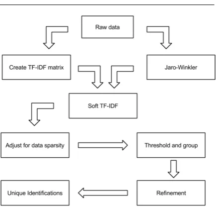
Fig. 2 shows an outline of our method. First we use TF-IDF to assign weights to features that in-dicate the importance of that feature in an entry. Next, we use soft TF-IDF with the Jaro-Winkler metric to address spelling inconsistencies in our
6 Our choice to normalize the rows ofTFIDFkby their
`1norms instead of their`2norms means that the
diag-onal elements ofTFIDFk TFIDFkT
[image:7.595.307.525.58.268.2]are not necessarily equal to 1.
Fig. 2: An outline of our method for duplicate de-tection
data sets. After this, we adjust for sparsity by tak-ing into consideration whether or not a record has missing entries. Using the similarity matrix pro-duced from the previous steps, we threshold and group records into clusters. Lastly, we refine these groups by evaluating how clusters break up under different conditions.
4.1 Adjusting for sparsity
A missing entry is an entry that is either entirely empty from the start or one that contains only null features and thus ends up being empty for our purposes. Here, we assume that missing en-tries do not provide any information about the record and therefore cannot aid us in determin-ing whether two records should be clustered to-gether (i.e. labeled as probable duplicates). In [65], [68], and [3], records with missing entries are dis-carded, filled in by human fieldwork, and filled in by an expectation-maximization (EM) imputation algorithm, respectively. For cases in which a large number of entries are missing, or in data sets with a large number of fields such that records have a high probability of missing at least one entry, these first two methods are impractical. Further-more, the estimation of missing fields is equiva-lent to unordered categorical estimation. In fields where a large number of features are present (i.e. the set of features is large), estimation by an EM scheme becomes computationally intractable [53] [70] [30]. Thus, a better method is required.
proceed. However, because the Jaro-Winkler met-ric between a null feature and any other feature is 0, the soft TF-IDF score between a missing en-try and any other enen-try is 0. This punishes sparse records in the composite soft TF-IDF similarity score matrixST. Even if two records have the ex-act same entries in fields where both records do not have missing entries, their missing entries deflate their composite soft TF-IDF similarity. Consider the following example using two records (from a larger data set containingn >2 records) and three fields: [“Joe Bruin”, “ ”, “male”] and [“Joe Bruin’, “CA”, “ ”]. The two records are likely to represent a unique entity “Joe Bruin”, but the composite soft TF-IDF score between the two records is on the lower end of the similarity score range (1 out of a maximum of 3) due to the missing entry in the second field for the first record and the missing entry in the third field for the second record. The issue described above for the soft TF-IDF method is also present for the TF-IDF method described in Section 3.4.
To correct for this, we take into consideration the number of mutually present (not missing) en-tries in the same field for two records. This can be done in a vectorized manner to accelerate compu-tation. Let B be then×abinary matrix defined by
Bi,k :=
(
0, ifei,k is a missing entry, 1, otherwise.
This is a binary mask of the data set, where 1 denotes a non-missing entry (with or without error), and 0 denotes a missing entry. In the prod-uctBBT ∈
Rn×n, each (BBT)i,j is the number of “shared fields” between recordsri andrj, i.e. the number of fieldscksuch that bothei,k andej,kare non-missing entries. Our adjusted (soft) TF-IDF similarity score is given by
adjSTi,j:=
STi,j
(BBT)
i,j, ifi6=j and (BB
T) i,j6= 0, 0, ifi6=j and (BBT)
i,j= 0, 1, ifi=j.
(6)
Remembering thatJW(fk
p, fqk) = 0 iffpk is a null feature or fk
q is a null feature, we see that, if ei,k is a missing entry or ej,k is a missing entry, then the setSk
i,j(θ) used in (3) is empty (independent of the choice ofθ) and thussTFIDFk
i,j= 0. The same conclusion is true in (5) since theith orjth row of TFIDFk consists of zeros in that case. Hence, we have that, for alli, j(i6=j), (ST)i,j∈[0,(BBT)i,j] (which refines our earlier result that (ST)i,j ∈[0, a]) and thus (adjST)i,j∈[0,1].
In the event that there are records ri and rj such that (BBT)
i,j= 0, it follows thatSTi,j= 0. Hence it makes sense to defineadjSTi,j to be zero in this case. In the data sets we will discuss in Section 5, no pair of records was without shared fields. Hence we can use the shorthand expression adjST =STBBT for our purposes in this paper7, wheredenotes element-wise division.
Algorithm 4: Adjusting for Sparsity
Data:sTFIDFk∈
Rn×n fork∈ {1, . . . , a},Dan n×aarray of text
Result:adjST ∈Rn×n
foreach entryei,kin each fieldckofDdo ComputeBi,k
end
InitializeST =P
ksTFIDFk
AdjustST for sparsity: adjST =STBBT
Instead of the method proposed above to deal with missing data, we can also perform data im-putation to replace the missing data with a “likely candidate” [35, 36, 4, 31, 40, 66]. To be precise, be-fore computing the matrixB, we replace each miss-ing entryei,kby the entry which appears most of-ten in the kth field8. In case of a tie, we choose an entry at random among all the entries with the most appearances (we choose this entry once per field, such that each missing entry in a given field is replaced by the same entry). For a clean com-parison, we still compute the matrixB(which has now no 0 entries) and use it for the normalization in (6). The rest of our method is then implemented as usual. We report the results of this comparison in Section 5.4.
4.2 Thresholding and grouping
The similarity scoreadjSTi,jgives us an indication of how similar the recordsri andrj are. IfadjSTi,j is close to 1, then the records are more likely to represent the same entity. Now, we present our method of determining whether a set of records
7 Since we defined the inconsequential diagonal
en-tries to besTFIDFk
i,i= 1 in (3) and (5), it could be that (ST)i,i>(BBT)i,ifor somei, which is why we explic-itly defined (adjST)i,i = 1 in (6) for consistency with the other values. Since the diagonal values will play no role in the eventual clustering this potential discrepancy between (6) andadjST =STBBT is irrelevant for our purposes.
8 We use the mode, rather than the mean, because all
are duplicates of each other based onadjST. There exist many clustering methods that could be used to accomplish this goal. For example, [46] considers this question in the context of duplicate detection. For simplicity, in this paper we restrict ourselves to a relatively straightforward thresholding proce-dure, but other methods could be substituted in future implementations. We call this the thresh-olding and grouping step (TGS).
The method we will present below is also appli-cable to clustering based on other similarity scores. Therefore it is useful to present it in a more general format. LetSIM ∈Rn×n be a matrix of similarity scores, i.e., for alli, j, the entrySIMi,jis a similar-ity score between the recordsriandrj. We assume that, for all i 6= j, SIMi,j = SIMj,i ∈ [0, a]9. If we use our adjusted (soft) TF-IDF method, SIM is given by adjST from (6). In Section 4.1 we saw that in that case we even haveSIMi,j∈[0,1].
Let τ ∈ [0, a] be a threshold and let S be the thresholded similarity score matrix defined fori6= j as
Si,j:=
(
1, ifSIMi,j≥τ, 0, ifSIMi,j< τ.
The outcome of our method does not depend on the diagonal values, but for definiteness (and to simplify some computations) we set Si,i := 1, for all i. If we want to avoid trivial clusterings (i.e. with all records in the same cluster, or with each cluster containing only one record) the threshold valueτ must be chosen in the half-open interval
min
i,j:j6=iSIMi,j,i,j:jmax6=iSIMi,j
.
If Si,j = 1, then the records ri and rj are clustered together. Note that this is a sufficient, but not necessary condition for two records to be clustered together. For example, if Si,j = 0, but
Si,k = 1 and Sj,k = 1, then ri and rk are clus-tered together, as arerj andrk, and thus so areri and rj. The output of the TGS is a clustering of all the records in the data set, i.e. a collection of clusters, each containing one or more records, such that each record belongs to exactly one cluster.
The choice of τ is crucial in the formation of clusters. Choosing a threshold that is too low leads to large clusters of records that represent more than one unique entity. Choosing a threshold that is too high breaks the data set into a large number
9 We will not be concerned with the diagonal values
ofSIM, because trivially any record is a ‘duplicate’ of itself, but for definiteness we may assume that, for alli,
SIMi,i=a.
of clusters, where a single entity may be repre-sented by more than one cluster. Here, we propose a method of choosingτ.
LetH ∈Rn be then×1 vector defined by
Hi:= max 1≤j≤n
j6=i
SIMi,j.
In other words, the ith element ofH is the maxi-mum similarity scoreSIMi,jbetween theithrecord and every other record. Now define
τH:=
(
µ(H) +σ(H),ifµ(H) +σ(H)<maxiHi,
µ(H), else,
where µ(H) is the mean value of H and σ(H) is its corrected sample standard deviation10.
We chooseτH in this fashion, because it is eas-ily implementable, has shown to work well in prac-tice (see Section 5) even if it is not always the optimal choice, and is based on some underlying heuristic ideas and empirical observations of the statistics ofH in our data sets (which we suspect to be more generally applicable to other data sets) that we will explain below. It provides a good al-ternative to trial-and-error attempts at finding the optimalτ, which can be quite time-intensive.
For a given record ri, the top candidates to be duplicates ofri are those records rj for which
SIMi,j=Hi. A typical data set, however, will have many records that do not have duplicates at all. To reflect this, we do not want to set the thresholdτH lower thanµ(H). IfHis normally distributed, this will guarantee that at least approximately half of the records in the data set will not be clustered together with any other record. In fact, in many of our runs (Fig. 3a is a representative example), there is a large peak ofH values around the mean valueµ(H). ChoosingτHequal toµ(H) in this case will lead to many of the records corresponding to this peak being clustered together, which is typi-cally not preferred. Choosing τH =µ(H) +σ(H) will place the threshold far enough to the right of this peak to avoid overclustering, yet also far enough removed from the maximum value ofH so that not only the top matches get identified as du-plicates. In some cases, however, the distribution of H values has a peak near the maximum value instead of near the mean value (as, for example, in Fig. 3b) and the valueµ(H) +σ(H) will be larger than the maximumH value. In those cases we can choseτH =µ(H) without risking overclustering.
It may not always be possible to choose a thresh-old in such a way that all the clusters generated by our TGS correspond to sets of actual duplicates, as
(a)H corresponding to the TF-IDF method (with word feature, without refinement step, see Sec-tion 4.3) applied to the FI data set. The red line is the chosen valueτH=µ(H) +σ(H); the blue line indicatesµ(H).
[image:10.595.82.269.75.222.2](b) H corresponding to the soft TF-IDF method (with 3-gram features, with refinement, see Sec-tion 4.3) applied to the RST data set. The blue line indicates the chosen valueτH =µ(H); the red line indicatesµ(H) +σ(H).
Fig. 3: Histograms ofH for different methods ap-plied to the FI and RST data sets (see Section 5.1)
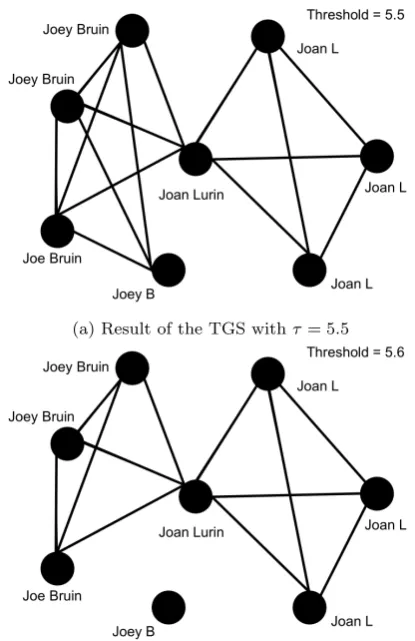
the following example, illustrated in Fig. 4, shows. We consider an artificial toy data set for which we computed the adjusted soft TF-IDF similarity, based on seven fields. We represent the result of the TGS as a graph in which each node represents a record in the data set. We connect nodes i and j (i6=j) by an edge if and only if their similarity scoreSIMi,j equals or exceeds the chosen thresh-old valueτ. The connected components of the re-sulting graph then correspond to the clusters the TGS outputs.
For simplicity, Fig. 4 only shows the features of each entry from the first two fields (first name and last name). Based on manual inspection, we declare the ground truth for this example to con-tain two unique entities: “Joey Bruin” and “Joan Lurin”. The goal of our TGS is to detect two clus-ters, one for each unique entity. Using τ = 5.5,
we find one cluster (Fig. 4a). Using τ = 5.6, we do obtain two clusters (Fig. 4b), but it is not true that one cluster represents “Joey Bruin” and the other “Joan Lurin”, as desired. Instead, one clus-ters consists of only the “Joey B” record, while the other cluster contains all other records. Increasing τ further until the clusters change, would only re-sult in more clusters, therefore we cannot obtain the desired result this way. This happens because the adjusted soft TF-IDF similarity between “Joey B” and “Joey Bruin” (respectively “Joe Bruin”) is less than the adjusted soft TF-IDF similarity between “Joey Bruin” (respectively “Joe Bruin”) and “Joan Lurin”. To address this issue, we apply a refinement step to each set of clustered records created by the TGS, as explained in the next sec-tion.
The graph representation of the TGS output turns out to be a very useful tool and we will use its language in what follows interchangeably with the cluster language.
Algorithm 5: Thresholding and grouping
Data:SIM=ST ∈Rn×n, threshold valueτ
(manual choice or automaticτ=τH)
Result:a collection ofcclustersC={R1. . . Rc}
foreachido
InitializeSi,i= 1
end
foreach pair of distinct recordsri andrj do ComputeSi,j
end
foreach pair of distinct recordsri andrj do IfSi,j= 1, assignriandrj to the same
cluster
end
4.3 Refinement
As the discussion of the TGS and the example in Fig. 4 have shown, the clusters created by the TGS are not necessarily complete subgraphs: it is possi-ble for a cluster to contain recordsri,rj for which
Si,j = 0. In such cases it is a priori unclear if the best clustering is indeed achieved by grouping ri andrj together or not. We introduce a way to re-fine clusters created in the TGS, to deal with sit-uations like these. We take the following steps to refine a cluster R:
[image:10.595.91.271.284.425.2](a) Result of the TGS withτ = 5.5
[image:11.595.75.283.70.391.2](b) Result of the TGS withτ= 5.6
Fig. 4: Two examples of clusters created by the TGS applied to an artificial data set, with different threshold valuesτ
2. ifRneeds be to refined, remove one record at a time from Rto determine the ‘optimal record’ r∗to remove;
3. if r∗ is removed from R, find the subcluster that r∗ does belong to.
Before we describe these steps in more detail, we introduce more notation. Given a cluster (as deter-mined by the TGS)R ={rt1, . . . , rtp} containing precords, the thresholded similarity score matrix of the cluster R is given by the restricted matrix S|R ∈ Rp×p with elements (S|R)i,j := Sti,tj. Re-member we represent R by a graph, where each node corresponds to a recordrti and two distinct nodes are connected by an edge if and only if their corresponding thresholded similarity score (S|R)i,j is 1. If a recordrti is removed fromR, the remain-ing set of records is
R(rti) := {rt1, . . . , rti−1, rti+1, . . . , rtp}. We define thesubclusters R1, . . . Rq ofR(rti) as the subsets of nodes corresponding to the connected compo-nents of the subgraph induced byR(r(ti)).
Step 1. Starting with a cluster R from the TGS, we first determine ifR needs to be refined, by in-vestigating, for each rti ∈ R, the subclusters of R(rti). If, for every rti ∈ R, R(rti) has a single subcluster, thenRneed not be refined. An exam-ple of this is shown in Fig. 5. If there is anrti∈R, such thatR(rti) has two or more subclusters, then we refineR.
Step 2. For any set ˜R consisting ofprecords, we define its strength as the average similarity be-tween the records in ˜R:
s( ˜R) :=
p
P
i,j=1 i6=j
(S|R˜)i,j
(p 2)
, ifp≥2,
0, ifp= 1.
(7)
Note that s( ˜R) = 1 if S|R˜ = 1
p×p (it suffices if the off-diagonal elements satisfy this equality). In other words, a cluster has a strength of 1 if ev-ery pair of distinct records in that cluster satisfy condition 1 of the TGS.
If in Step 1 we have determined that the cluster R requires refinement, we find the optimal record r∗ :=rtk∗ such that the average strength of sub-clusters ofR(r∗) is maximized:
k∗= arg max 1≤i≤p
1 q(i)
q(i)
X
j=1
s(Rj).
Here the sum is over alljsuch thatRjis a subclus-ter ofR(rti), andq(i) is the (i-dependent) number of subclusters ofR(rti). In the unlikely event that the maximizer is not unique, we arbitrarily choose one of the maximizers ask∗. Since the strength of a subcluster measures the average similarity be-tween the records in that subcluster, we want to keep the strength of the remaining subclusters as high as possible after removing r∗ and optimizing the average strength is a good strategy to achieve that.
Step 3. After finding the optimal r∗ to remove, we now must determine the subcluster to which to add it. We again use the strength of the resulting subclusters as a measure to decide this. We eval-uate the strength of the set Rj ∪ {r∗} ⊂ R, for each subcluster Rj ⊂ R(r∗). We then add r∗ to subclusterRl∗ to formR∗:=Rl∗∪ {r∗}, where
l∗:= arg max j:Rjis a subcluster
ofR(r∗)
s(Rj∪ {r∗}).
Fig. 5: An example of a clusterRthat does not require refinement. Each node represents a record. In each test we remove one and only one node from the cluster and apply TGS again. The red node represents the removed record rti, the remaining black nodes make up the set R(ti). Notice that every time we remove a record, all other records are still connected to each other by solid lines, henceRdoes not need to be refined.
We always addr∗ to one of the other subclus-ters and do not consider the possibility of letting {r∗} be its own cluster. Note that this is justi-fied, since from our definition of strength in (7), s({r∗}) = 0< s(R∗), becauser∗was connected to at least one other record in the original clusterR.
Finally, the original clusterR is removed from the output clustering, and the new clusters R1, . . . , Rl∗−1, R∗, Rl∗+1, . . . , Rq(k∗) are added to
[image:12.595.306.522.346.669.2]the clustering.
Fig. 6 shows an example of how the refinement helps us to find desired clusters.
Algorithm 6: Refinement
Data:R={rt1, . . . , rtn}a cluster resulting from the TGS
Result:Rset of refined clusters
if there exists rti such thatR(rti)has more than 1 subclusterthen
foreachrti∈Rdo
Find the subclusters R1, . . . Rq ofR(rti) Compute 1
q Pq
j=1s(Rj)
end
Assign r∗=r
tk∗ where
k∗= arg max
i
1
q Pq
j=1s(Rj)
foreach subclusterRi⊂R(r∗)do Computes(Ri∪ {r∗})
end
Assign R∗= (Rl∗∪ {r∗})where
l∗= arg maxjs(Rj∪ {r∗})
R={R1, . . . , Rl∗−1, Rl∗, Rl∗+1, . . . , Rq(k∗)}
end else
Do not refine R:R={R}
end
[image:12.595.74.289.534.766.2]In our implementation, we computed the opti-mal valuesk∗ and l∗ are via an exhaustive search over all parameters. This can be computationally expensive when the initial threshold τ is small, leading to large initial clusters.
We only applied the refinement step process once (i.e., we executed Step 1 once and for each cluster identified in that step we applied Steps 2 and 3 once each). It is possible to iterate this three step process until no more ‘unstable’ clusters are found in Step 1.
5 Results 5.1 The data sets
The results presented in this section are based on four data sets: the Field Interview Card data set (FI), the Restaurant data set (RST), the Restau-rant data set with entries removed to induce spar-sity(RST30), and theCora Citation Matching data set (Cora). FI is not publicly available. The other data sets currently can be found at [55]. Cora can also be accessed at [6]. RST and Cora are also used in [10] to compare several approaches to evaluate duplicate detection.
FI This data set consists of digitizedField Inter-view cards from the LAPD. Such cards are cre-ated at the officer’s discretion whenever an inter-action occurs with a civilian. They are not re-stricted to criminal events. Each card contains 61 fields of which we use seven: last name, first name, middle name, alias/moniker, operator licence num-ber (driver’s licence), social security numnum-ber, and date of birth. A subset of this data set is used and described in more detail in [25]. The FI data set has 8,834 records, collected during the years 2001–2011. A ground truth of unique individuals is available, based on expert opinion. There are 2,920 unique people represented in the FI data set. The FI data set has many misspellings as well as differ-ent names that correspond to the same individual. Approximately 30% of the entries are missing, but the “last name” field is without missing entries.
RST This data set is a collection of restaurant in-formation based on reviews fromFodor andZagat, collected by Dr. Sheila Tejada [62], who also man-ually generated the ground truth. It contains five fields: restaurant name, address, location, phone number, and type of food. There are 864 records containing 752 unique entities/restaurants. There are no missing entries in this data set. The types
of errors that are present include word and let-ter transpositions, varying standards for word ab-breviation (e.g. “deli” and “delicatessen”), typo-graphical errors, and conflicting information (such as different phone numbers for the same restau-rant).
RST30 To be able to study the influence of spar-sity of the data set on our results, we remove ap-proximately 30% of the entries from the address, city, phone number, and type of cuisine fields in the RST data set. The resulting data set we call RST30. We choose the percentage of removed en-tries to correspond to the percentage of missing entries in the FI data set. Because the FI data set has a field that has no missing entries, we do not remove entries from the “name” field.
Cora The records in the Cora Citation Matching data set11 are citations to research papers [44]. Each of Cora’s 1,295 records is a distinct citation to any one of the 122 unique papers to which the data set contains references. We use three fields: author(s), name of publication, and venue (name of the journal in which the paper is published). This data set contains misspellings and a small amount of missing entries (approximately 3%).
5.2 Evaluation metrics
We compare the performances of the methods sum-marized in Table 1. Each of these method outputs a similarity matrix, which we then use in the TGS to create clusters.
To evaluate the methods, we usepurity[28], in-verse purity, theirharmonic mean[26], therelative error in the number of clusters, precision, recall [17, 11], theF-measure(orF1score) [56, 7],z-Rand score [45, 63], andnormalized mutual information (NMI) [60], which are all metrics that compare the output clusterings of the methods with the ground truth.
Purity and inverse purity compare the clusters of records which the algorithm at hand gives with the ground truth clusters. Let C :={R1, . . . , Rc} be the collection ofcclusters obtained from a clus-tering algorithm and let C0 := {R0
1, . . . , R0c0} be
the collection of c0 clusters in the ground truth. Remember thatnis the number of records in the data set. Then we definepurity as
Pur(C,C0) := 1 n
c
X
i=1 max
1≤j≤c0|Ri∩R
0 j|,
11 The Cora data set should not be confused with the
where we use the notation|A|to denote the cardi-nality of a setA. In other words, we identify each clusterRiwith (one of the) ground truth cluster(s)
R0jwhich shares the most records with it, and com-pute purity as the total fraction of records that is correctly classified in this way. Note that this mea-sure is biased to favor many small clusters over a few large ones. In particular, if each record forms its own cluster,Pur = 1. To counteract this bias, we also considerinverse purity,
Inv(C,C0) :=Pur(C0,C) = 1 n
c0
X
i=1 max 1≤j≤c|R
0 i∩Rj|.
Note that inverse purity has a bias that is opposite to purity’s bias: if the algorithm outputs only one cluster containing all the records, thenInv = 1.
We combine purity and inverse purity in their harmonic mean12,
HM(C,C0) := 2Pur×Inv Pur+Inv .
The relative error in the number of clusters in C is defined as
|C| − |C0|
|C0| = |c−c0|
c0 .
We define precision, recall, and the F-measure (or F1 score) by consideringpairs of clusters that have correctly been identified as duplicates. This differs from purity and inverse purity as defined above, which consider individual records. To define these metrics the following notation is useful. Let G be the set of (unordered) pairs of records that are duplicates, according to the ground truth of the particular data set under consideration,
G:=
{r, s}:r6=sand∃R0∈ C0 s. t.r, s∈R0},
and let C be the set of (unordered) record pairs that have been clustered together by the duplicate detection method of choice,
C:=
{r, s}:r6=sand∃R∈ C s. t.r, s∈R .
Precisionis the fraction of the record pairs that have been clustered together that are indeed du-plicates in the ground truth,
Pre(C,C0) :=|C∩G| |C| ,
12 The harmonic mean of purity and inverse purity is
sometimes also called the F-score or F1-score, but we will refrain from using this terminology to not create confusion with the harmonic mean of precision and re-call.
and recall is the fraction of record pairs that are duplicates in the ground truth that have been cor-rectly identified as such by the method
Rec(C,C0) := |C∩G| |G| .
TheF-measure or F1 score is the harmonic mean of precision and recall,
F(C,C0) := 2Pre(C,C
0)×Rec(C,C0) Pre(C,C0) +Rec(C,C0) = 2
|C∩G| |G|+|C|.
Note that in the extreme case in which|C|=n, i.e. the case in which each cluster contains only one record, precision, and thus also the F-measure, are undefined.
Another evaluation metric based on pair count-ing, is the z-Rand score. The z-Rand score zR is the number of standard deviations by which|C∩G| is removed from its mean value under a hyperge-ometric distribution of equally likely assignments with the same number and sizes of clusters. For further details about the z-Rand score, see [45, 63, 25]. The relative z-Rand score of C is the z -Rand score of that clustering divided by the z -Rand score of C0, so that the ground truthC0 has a relativez-Rand score of 113.
A final evaluation metric we consider, is nor-malized mutual information(NMI). To define this, we first need to introduce mutual information and entropy. We define theentropy of the collection of clustersC as
Ent(C) :=− c
X
i=1 |Ri|
n log |R
i|
n
, (8)
and similarly for Ent(C0). The joined entropy ofC andC0 is
Ent(C,C0) :=− c
X
i=1 c0
X
j=1
|Ri∩R0j|
n log
|R
i∩Rj0|
n
.
Themutual informationofCandC0is then defined as
I(C,C0) :=Ent(C) +Ent(C0)−Ent(C,C0)
= c
X
i=1 c0
X
j=1
|Ri∩R0j|
n log
n|R
i∩R0j| |Ri||Rj|
,
where the right hand side follows from the equal-itiesPc
i=1|Ri∩R0j|=|R0j| and
Pc0
j=1|Ri∩R0j|= |Ri|. There are various ways in which mutual infor-mation can be normalized. We choose to normalize
13 We conjecture that the relative z-Rand score is
by the geometric mean of Ent(C) and Ent(C0) to give thenormalized mutual information
NMI(C,C0) := I(C,C 0)
p
Ent(C)Ent(C0).
Note that the entropy of C is zero, and hence the normalized mutual information is undefined, when |C|= 1, i.e. when one cluster contains all the records. In practice this is avoided by adding a small num-ber (e.g. the floating-point relative accuracy eps
in MATLAB) to the argument of the logarithm in (8) forEnt(C) andEnt(C0).
Because we are testing our methods on data sets for which we have ground truth available, the metrics we use all compare our output with the ground truth. This would not be an option in a typical application situation in which the ground truth is not available. If the methods give good re-sults in test cases in which comparison with the ground truth is possible, it increases confidence in the methods in situations with an unknown ground truth. Which of the metrics is the most appropri-ate in any given situation depends on the needs of the application. For example, in certain situations (for example when gathering anonymous statis-tics from a data set) the most important aspect to get right might be the number of clusters and thus the relative error in the number of clusters metric would be well suited for use, whereas in other situations missing out on true positives or including false negatives might carry a high cost, in which case precision or recall, respectively, or theF1 score are relevant metrics. For more infor-mation on many of these evaluation metrics, see also [5].
5.3 Results
In this section we consider six methods: TF-IDF, soft TF-IDF without the refinement step, and soft TF-IDF with the refinement step, with each of these three methods applied to both word features and 3-gram features. We also consider five evalu-ation metrics: the harmonic mean of purity and inverse purity, the relative error in the number of clusters, the F1 score, the relative z-Rand score, and the NMI. We investigate the results in two dif-ferent ways: (a) by plotting the scores for a partic-ular evaluation metric versus the threshold values, for the six different methods in one plot and (b) by plotting the evaluation scores obtained with a particular method versus the threshold values, for all five evaluation metrics in one plot. Since this paper does not offer space to present all figures,
Name Similarity Features Ref. matrix
TFIDF ST using (5) words no
[image:15.595.310.522.68.156.2]TFIDF 3g ST using (5) 3-grams no sTFIDF ST using (3) words no sTFIDF 3g ST using (3) 3-grams no sTFIDF ref ST using (3) words yes sTFIDF 3g ref ST using (3) 3-grams yes
Table 1: Summary of methods used. The second, third, and fourth columns list for each method which similarity score matrix is used in the TGS, if words or 3-grams are used as features, and if the refinement step is applied after TGS or not, re-spectively. Equation (4) is always used to compute the similarity score, but the important difference is whether the soft TF-IDF matrix from (3) or the TF-IDF matrix from (5) is used in (4).
we show some illustrative plots and describe the main results in the text. In Section 6 we will dis-cuss conclusions based on these results.
5.3.1 The methods
When we compare the different methods by plot-ting the scores for a particular evaluation met-ric versus the threshold value τ for all the meth-ods in one plot (as can be seen for example in Fig. 7a), one notable attribute is that the behav-ior of the methods that use word features typically is quite distinct from that of the methods that use 3-gram features. This is not very surprising, since the similarity scores produced by those methods, and hence their response to different threshold val-ues, are significantly different.
It is also interesting to note which methods give better evaluation metric outcomes on which data sets. First we compare the word based methods with the 3-gram based methods. On the FI data set the word feature based methods outperform the 3-gram based methods (judged on the basis of best case performance, i.e. the optimal score attained over the full threshold range) for every evaluation metric by quite a margin, except for the NMI for which the margin is minimal (but still extant).
On both the RST and RST30 data sets, the word feature based methods outperform the 3-gram feature based methods on the pair counting based metrics, i.e. F1 score and relative z-Rand score (Fig. 7b), but both groups of methods perform equally well for the other metrics.
(a) TheF1 score for the Cora data set
[image:16.595.84.289.66.429.2](b) The relativez-Rand score for the RST data set
Fig. 7: Two evaluation metrics as a function of the threshold valueτ, computed on two different data sets. Each of the six graphs in a plot correspond to one of the six methods used. The filled markers in-dicate the metric’s value at the automatically cho-sen threshold valueτH for each method. In the leg-end, “(s)TF-IDF” stands for (soft) TF-IDF, “3g” indicates the use of 3-gram based features instead of word based ones, and “ref” indicates the pres-ence of the refinement step.
the other data sets. The difference in the relative error in the number of clusters is more pronounced however, in favor of the former method. Only on the relative error in the number of clusters does it perform somewhat worse than sTIDF ref. In fact, on all other metrics sTFIDF 3g ref outperforms the other two word based methods (TFIDF and sTFIDF). The other 3-gram based methods per-form worse than their word based counterparts on the pair counting metrics and on par with them on the other metrics.
Next we compare the TF-IDF methods with the soft TF-IDF methods (without refinement step in all cases). There are very few observable
differ-ences between TFIDF 3g and sTFIDF 3g in any of the metrics or data sets, and where there are, the differences are minor.
The comparison between TFIDF and sTFIDF shows more variable behavior. The most common behavior among all metrics and data sets is that both methods perform equally well in the regions with very small or very large values ofτ, although in some cases these regions themselves can be very small indeed. In the intermediate region, TFIDF usually performs better at smallτ values, whereas sTFIDF performs better at larger τ values. The size of the these different regions, as well as the size of the difference in outcome can differ quite substantially per case. For example, in the case of NMI for the Cora data set, NMI and the harmonic mean of purity and inverse purity for the RST data set, and all metrics except the relative error in the number of clusters for the RST30 data set, TFIDF outperforms sTFIDF quite consistently in the re-gions where there is a difference.
When it comes to the benefits of including the refinement step, the situation is again somewhat different depending on the data set. First we com-pare sTFIDF 3g with sTFIDF 3g ref. For small threshold values including the refinement step is beneficial (except in a few cases when there is little difference for very smallτvalues). This is to be ex-pected, since the refinement will either increase the number of clusters formed or keep it the same, so its effect is similar to (but not the same as) raising the threshold value. For larger τ values typically one of two situations occurs: either sTFIDF 3g out-performs sTFIDF 3g ref for intermediateτ values and there is little difference for higherτ values, or there is little difference on the whole range of in-termediate and large τ values. The former occurs to a smaller or larger degree for all metrics except NMI for the Cora data set, for the harmonic mean of purity and inverse purity and the relative error in the number of clusters for the FI data set, and also for the relative error in the number of clusters for the RST30 data set. The other cases display the second type of behaviour.
set), or by a region of the remaining intermediate and large τ values in which both methods are on par (NMI for the Cora data set, the F1 score, the harmonic mean of purity and inverse purity, and NMI for the RST30 data set, and all metrics for the RST data set), or by first a region of inter-mediate τ values on which sTFIDF outperforms sTFIDF ref, followed by a region on which there is little difference between the methods (all other metric/data set combinations).
It is also noteworthy that all methods do signif-icantly worse on RST30 than on RST, when mea-sured according to the pair counting based meth-ods (theF1and relativez-Rand scores), while there is no great difference, if any, measured according to the other metrics. In this context it is interesting to remember that RST30 is created by removing 30% of the entries from all but one of the fields of RST.
5.3.2 The metrics
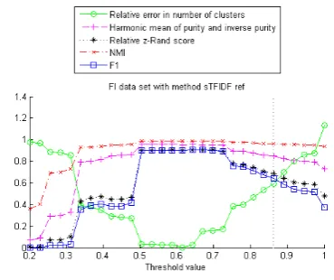
[image:17.595.327.512.71.225.2]When plotting the different evaluation metrics per method, we notice that the two pair counting based metrics, i.e. theF1score and relativez-Rand score, behave similarly to each eather, as do the harmonic mean of purity and inverse purity and the NMI. The relative error in the number of clusters is cor-related to those other metrics in an interesting way. For the word feature based methods, the lowest relative error in the number of clusters is typically attained at or near the threshold values at which theF1and relativez-Rand scores are highest (this is much less clear for the Cora data set as it is for the others). Those are also usually the lowest threshold values for which the harmonic mean and NMI attain their high(est) values. The harmonic mean and NMI, however, usually remain quite high when the threshold values are increased, whereas the F1 and relative z-Rand scores typically drop (sometimes rapidly) at increased threshold values, as the relative error in number of clusters rises. Fig. 8a shows an example of this behavior.
The relationship between the harmonic mean of purity and inverse purity and the NMI has some interesting subtleties. As mentioned before they mostly show similar behavior, but the picture is slightly more subtle in certain situations. On the Cora data set, the harmonic mean drops noticeably for higher threshold values, before settling eventu-ally at a near constant value. This is a drop that is not present in the NMI. This behavior is also present in the plots for the 3-gram feature based methods on the FI data set and very slightly in the word feature based methods on the RST data set (but not the RST30 data set). For word feature
(a) Soft TF-IDF (on word based features) without the refinement step applied to the RST30 data set
(b) Soft TF-IDF (on word based features) with the refinement step applied to the FI data set
Fig. 8: Different evaluation metrics as a function of the threshold value τ, computed on two different data sets. Each of the five graphs in a plot corre-spond to one of five evaluation metrics. The verti-cal dotted line indicates the automativerti-cally chosen threshold value τH for the method used.
based methods on the FI data set the behavior is even more pronounced, with little to no ‘set-tling down at a constant value’ happening for high threshold values (e.g. Fig. 8b).
Interestingly, both the harmonic mean and NMI show very slight (but consistent over both data sets) improvements at the highest threshold val-ues for the 3-gram based methods applied to the RST and RST30 data sets.
[image:17.595.324.509.255.410.2]in two entries, but also from features that are very similar. Hence the soft TF-IDF similarity score be-tween two entries will be higher than the TF-IDF score between the same entries and thus clusters are less likely to break up at the same τ value in the soft TF-IDF method than in the TF-IDF method. For τ values less than the optimal value the breaking up of clusters is beneficial, as the op-timal cluster number has not yet been reached and thus TFIDF will outperform sTFIDF on the rela-tive error in the number of clusters metric in this region. For τ larger than the optimal value, the situation is reversed.
5.3.3 The choice of threshold
On the RST and RST30 data sets our automati-cally chosen threshold performs well (e.g. see Figs. 7b, 8a, and 9a). It usually is close to (or sometimes even equal to) the threshold value at which some or all evaluation metrics attain their optimal value (remember this threshold value is not the same for all the metrics). The performance on RST is slightly better then on RST30, as can be expected, but in both cases the results are good.
On the FI and Cora data sets our automati-cally chosen threshold is consistently larger than the optimal value, as can be seen in e.g. Figs. 7a, 8b, and 9b. This can be explained by the left-skewedness of the H-value distribution, as illus-trated in Fig. 3a. A good proxy for the volume of the tail is the ratio of number of records referring to unique entities to the total number of entries in the data set. For RST and RST30 this ratio is a high 0.87, whereas for FI it is 0.33 and for Cora only 0.09. This means that the relative error in the number of clusters grows rapidly with increasing threshold value and the values of the other evalu-ation metrics will deteriorate correspondingly.
We also compared whether TFIDF, sTFIDF, or sTFIDF ref performed better at the value τ = τH. Interestingly, sTFIDF ref never outperformed all the other methods. At best it tied with other methods: for theF1and relativez-Rand scores for the RST30 data set it performed equally well as TFIDF; all three methods performed equally well for the NMI for the Cora data set, for the NMI and relative error in the number of clusters for the RST data set, and for NMI and the harmonic mean of the purity and inverse purity for the RST30 data set. TFIDF and sTFIDF tied for the F1 and rel-ative z-Rand scores for the FI data set. TFIDF outperformed the other methods on the RST data set for the F1 and relative z-Rand scores, as well as the harmonic mean of purity and inverse purity. Finally, sTFIDF outperformed the other methods
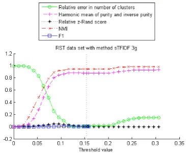
(a) Soft TF-IDF (on 3-gram based features) without the refinement step applied to the RST data set
(b) Soft TF-IDF (on 3-gram based features) with the refinement step applied to the FI data set
Fig. 9: Different evaluation metrics as a function of the threshold value τ, computed on two different data sets. Each of the five graphs in a plot corre-spond to one of five evaluation metrics. The verti-cal dotted line indicates the automativerti-cally chosen threshold value for the method used.
across the board for the FI data set, as well as for all metrics but the NMI for the Cora data set and for the relative error in the number of clusters for the RST30 data set. To recap, atτ =τH, the soft TF-IDF method seems to be a good choice for the Cora and FI data set, while for most metrics for the RST and RST30 data sets the TF-IDF method is preferred atτ =τH. (Remember that the value
τH depends on the data set and the method).
5.4 Results for alternative sparsity adjustment
[image:18.595.327.510.74.224.2]