Galaxy Zoo: comparing the demographics of spiral arm number and a new method for correcting redshift bias

Galaxy Zoo: comparing the demographics of spiral arm number and a

new method for correcting redshift bias

Ross E. Hart,

Steven P. Bamford,

Kyle W. Willett,

Karen L. Masters,

Carolin Cardamone,

Chris J. Lintott,

Robert J. Mackay,

Robert C. Nichol,

Christopher K. Rosslowe,

Brooke D. Simmons

and Rebecca J. Smethurst

1_{School of Physics and Astronomy, The University of Nottingham, University Park, Nottingham NG7 2RD, UK} 2_{School of Physics and Astronomy, University of Minnesota, 116 Church St SE, Minneapolis, MN 55455, USA} 3_{Department of Physics and Astronomy, University of Kentucky, 505 Rose St., Lexington, KY 40506, USA}

4_{Institute for Cosmology and Gravitation, University of Portsmouth, Dennis Sciama Building, Burnaby Road, Portsmouth PO1 3FX, UK} 5_{Department of Math and Science, Wheelock College, 200 Riverway, Boston, MA 02215, USA}

6_{Oxford Astrophysics, Department of Physics, University of Oxford, Denys Wilkinson Building, Keble Road, Oxford OX1 3RH, UK} 7_{Center for Astrophysics and Space Sciences (CASS), Department of Physics, University of California, San Diego, CA 92093, USA}

Accepted 2016 June 29. Received 2016 June 29; in original form 2016 April 26

A B S T R A C T

The majority of galaxies in the local Universe exhibit spiral structure with a variety of forms. Many galaxies possess two prominent spiral arms, some have more, while others display a many-armed flocculent appearance. Spiral arms are associated with enhanced gas content and star formation in the discs of low-redshift galaxies, so are important in the understanding of star formation in the local universe. As both the visual appearance of spiral structure, and the mechanisms responsible for it vary from galaxy to galaxy, a reliable method for defining spiral samples with different visual morphologies is required. In this paper, we develop a new debiasing method to reliably correct for redshift-dependent bias in Galaxy Zoo 2, and release the new set of debiased classifications. Using these, a luminosity-limited sample of∼18 000 Sloan Digital Sky Survey spiral galaxies is defined, which are then further sub-categorized by spiral arm number. In order to explore how different spiral galaxies form, the demographics of spiral galaxies with different spiral arm numbers are compared. It is found that whilst all spiral galaxies occupy similar ranges of stellar mass and environment, many-armed galaxies display much bluer colours than their two-armed counterparts. We conclude that two-armed structure is ubiquitous in star-forming discs, whereas many-armed spiral structure appears to be a short-lived phase, associated with more recent, stochastic star-formation activity. Key words: methods: data analysis – galaxies: formation – galaxies: general – galaxies: spi-ral – galaxies: structure.

1 I N T R O D U C T I O N

Spiral galaxies are the most common type of galaxy in the lo-cal Universe, with as many as two-thirds of low-redshift galaxies exhibiting discs with spiral structure (Nair & Abraham2010; Lin-tott et al.2011; Willett et al.2013; Kelvin et al. 2014a). As star formation is enhanced in gas-rich disc galaxies (Schmidt 1959; Kennicutt1989; Kelvin et al.2014a) understanding spiral structure holds the key to understanding star formation in the local Universe, yet formulating a single theory to account for all spiral structure still remains elusive. The main theories for the occurrence of spiral

_{E-mail:[email protected]}

arm features in local galaxies initially focused on the idea of being caused by density waves in their discs (Lindblad1963; Lin & Shu 1964), but have since been superseded by theories that consider the effects of gravity and disc dynamics (Toomre1981; Sellwood & Carlberg1984), with most of the work to advance the field of spiral structure theory driven by simulation [e.g. Dobbs & Baba (2014) and references therein, and discussed further in Section 4]. Using observational studies to test these theories remains a challenge, as visual classifications of both the presence of spiral structure and de-tails of its features are required, which are difficult to obtain when considering the large samples provided by galaxy survey data.

An approach that has been successfully employed to visually clas-sify galaxies in large surveys is citizen science, which asks many volunteers to morphologically classify galaxies rather than relying

at University of Nottingham on January 5, 2017

http://mnras.oxfordjournals.org/

on a small number of experts. Sophisticated automated methods have also been developed for this purpose, (e.g. Huertas-Company et al. 2011; Davis & Hayes2014; Dieleman, Willett & Dambre 2015). However, these methods cannot currently completely repro-duce the results of visual classifications, particularly in low signal-to-noise images. They also require training sets, meaning that ‘by eye’ inspection methods are still a requirement. Galaxy Zoo 1 (GZ1; Lintott et al.2008,2011) was the first project to collect visual mor-phologies using citizen science, by classifying galaxies from the Sloan Digital Sky Survey (SDSS) as either ‘elliptical’ or ‘spiral’. Using this method, each galaxy is classified by several individuals, and a likelihood or ‘vote fraction’ of each galaxy having a partic-ular feature is assigned as the fraction of classifiers who saw that feature. GZ1 classifications collected in this way have been used to compare galaxy morphology with respect to colour (Bamford et al.2009; Masters et al.2010a,b), environment (Bamford et al. 2009; Skibba et al.2009; Darg et al.2010a,b), and star-formation properties (Tojeiro et al.2013; Schawinski et al.2014; Smethurst et al.2015).

Following from the success of GZ1, more detailed visual clas-sifications were sought, including the presence of bars, and spiral arm winding and multiplicity properties. Thus, Galaxy Zoo 2 (GZ2) was created (Willett et al.2013, hereafterW13), in which volun-teers were asked more questions about a subsample of GZ1 SDSS galaxies. The main difference between GZ2 and GZ1 was that vi-sual classifications were collected using a ‘question tree’ in GZ2, to gain a more exhaustive set of morphological information for each galaxy. GZ2 has already been used to compare the properties of spi-ral galaxies with or without bars (Masters et al.2011,2012; Cheung et al.2013), look for interacting galaxies (Casteels et al.2013), as well as looking for relationships between spiral arm structure and star formation (Willett et al. 2015). This ‘question tree’ method has since been used in a similar way to measure the presence of de-tailed morphological features in higher redshift galaxy surveys (e.g. Melvin et al.2014; Simmons et al.2014), and otherZOONIVERSE1

citizen science projects.

An issue that arises in both visual and automated methods of morphological classification is that detailed features are more diffi-cult to observe in lower signal-to-noise images (i.e. observed from a greater distance). In Galaxy Zoo, this has been termed as classifi-cation bias. It is imperative that classificlassifi-cation bias is removed from morphological data, as it leads to sample contamination from galax-ies being incorrectly assigned to some categorgalax-ies. This means that any observational differences between samples can be significantly reduced.

Classification bias manifested itself in GZ1 with galaxies at higher redshift having lower ‘spiral’ vote fractions, which were corrected using a statistical method (Bamford et al.2009). The ap-plication of a question tree in GZ2 to look for more detailed features means that correcting for biases is more complicated than in GZ1. In particular, there are questions with several possible answers, and debiasing one answer with respect to each of the others is therefore a more difficult process for GZ2.

The paper is organized as follows. In Section 2, the sample se-lection and galaxy data are described. In Section 3, we describe a new debiasing method that has been created to account for the clas-sification bias in the GZ2 questions with multiple possible answers. In Section 4, samples of GZ2 spiral galaxies are defined and sorted by arm multiplicity. This is a case where the new debiasing method

1_{https://www.zooniverse.org/}

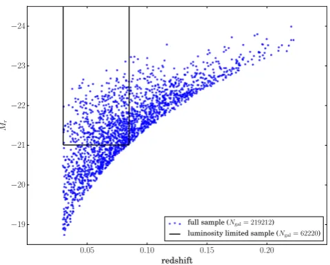
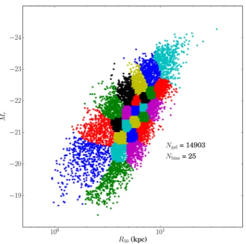
Figure 1. Ther-band luminosity versus redshift distribution of ourfull sample(blue points), with the region enclosing our 0.03< z <0.085,Mr≤ −21luminosity-limited sampleindicated by black lines.

is required as there are multiple responses to that question. Af-ter reviewing relevant theoretical and observational liAf-terature, we examine the demographics of spiral galaxies with respect to arm multiplicity, and begin to explore the processes that influence the formation and evolution of spiral arms in Section 4. The results are summarized in Section 5.

This paper assumes a flat cosmology withm=0.3 andH0=

70 km s−1_Mpc−1_.

2 DATA

2.1 Galaxy properties and sample selection

We make use of morphological information from the public data release of Galaxy Zoo 2. The galaxies classified by GZ2 were taken from the SDSS Data Release 7 (DR7; Abazajian et al.2009). The SDSS main galaxy sample is anr-band selected sample of galaxies in the legacy imaging area targeted for spectroscopic follow-up (Strauss et al.2002) The GZ2 sample contains essentially all well-resolved galaxies in DR7 down to a limiting absolute magnitude of

mr≤17, supplemented by additional sets of galaxies in Stripe 82 for

which deeper, co-added imaging exists (seeW13for details). In this paper, we only consider galaxies withmr≤17 that were classified

in normal-depth SDSS imaging and which have DR7 spectroscopic redshifts. We refer to this as ourfull sample, containing 228 201 galaxies, to which the debiasing procedure described in Section 3.3 is applied. We require redshifts in order to correct the sample for a distance-dependent bias, as described in Section 3.1.

Petrosian aperture photometry inugrizfilters is obtained from the SDSS DR7 catalogue. Rest-frame absolute magnitudes corrected for Galactic extinction are those computed by Bamford et al. (2009), usingKCORRECT(Blanton & Roweis2007). Galaxy stellar masses

are determined from ther-band luminosity andu−rcolour using the calibration adopted by Baldry et al. (2006).

In order to study galaxy properties in a representative manner in Section 4, we define aluminosity-limited samplewith 0.03< z < 0.085 andMr≤ −21, containing 62 220 galaxies. The luminosity

versus redshift distribution of our full sample, and the limits of ourluminosity-limited sample, are shown in Fig.1. These limits approximately maximize the sample size, given themr≤17 limit

at University of Nottingham on January 5, 2017

http://mnras.oxfordjournals.org/

on thefull sample. The lower redshift limit avoids a small number of galaxies with very large angular sizes, and hence accompanying morphological, photometric and spectroscopic complications. The upper redshift limit also corresponds to that for which we have reliable galaxy environmental density data from Baldry et al. (2006), which we will make use of in this paper.

The luminosity-limited sample is incomplete for the reddest galaxies at log (M/M) <10.6 (calculated using the method in Bamford et al.2009). Where necessary we therefore consider a

stellar mass-limited sampleof 41 801 galaxies, created by applying a limit of log (M/M)≥10.6 to theluminosity-limited sample.

2.2 Stellar population models

In Section 4.2.4, we evaluate potential star-formation histories by comparing observed galaxy colours. Spectral energy distributions are derived from Bruzual & Charlot (2003), for a range of ages and SFHs using the initial mass function from Chabrier (2003). For star-forming galaxies in the SDSS, the mean stellar metallicity varies fromZ≈0.7ZforM∼1010.6_M

(the lower limit of the stellar mass-limited sample) toZ≈ZforM∼1011_M

(Peng, Maiolino & Cochrane2015). As we expect most spirals to be blue star-forming galaxies (e.g. Bamford et al.2009), we approximate the metallicity of the stellar mass-limited spiral sample using a metallicity value ofZ=Z. Two dust extinction magnitudes ofAV =0 andAV=0.4 are considered (Calzetti et al.2000). Equivalent

colours for each of the star formation and dust extinction models are calculated for each of the SDSSugrizfilters (Doi et al.2010). Full details of how the models are derived can be found in Duncan et al. (2014).

2.3 Quantifying morphology with Galaxy Zoo

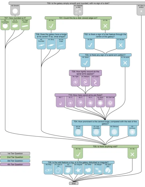
In GZ2, morphological information for each galaxy was obtained by asking participants to answer a series of questions. The structure of this question tree is shown in Fig. 2. Typically, each image was viewed by40 people (W13), although no user will explicitly answer every question in the tree for a particular galaxy. To reach the questions further down the tree, it is required that another question has been answered with a specific response. For each question, the responses are each represented by the ‘vote fraction’passigned to each possible answer. For any given question, the sum of the vote fractions for all possible answers adds up to one. Considering the ‘edge-on’ question (T01 in Fig.2), a classifier would only answer that question if they answered ‘features/disc’ for T00. For example; if a galaxy was classified by 40 people, and 30 of those said they saw features, whilst the other 10 claimed it was smooth, then the corresponding vote fractions arepfeatures=0.75 andpsmooth=0.25.

Only the 30 classifiers who saw ‘features’ would then answer the ‘edge-on’ question (T11 of Fig.2). If 15 of those said the galaxy was edge-on, and 15 said it was not, the corresponding vote fractions would bepedge-on=0.5 andpnot edge-on=0.5.

In order to reduce the influence of unreliable classifiers,W13 downweighted individual volunteers who had poor agreement with the other classifiers. Throughout this paper we refer to these weighted vote fractions as the ‘raw’ quantities. Before using these GZ2 vote fractions to study the galaxy population, we must first consider the issue of classification bias, as we shall in Section 3.1.

Traditional morphologies assign each galaxy to a specific class, usually determined by one, or occasionally a few, experts. In con-trast, Galaxy Zoo provides a large number of independent opinions on specific morphological features for each galaxy. This allows us to

consider both the inherent ‘subjectiveness’ and observational uncer-tainties of galaxy morphology, and hence control the compromise between sample contamination and completeness.

There are two principal ways in which galaxy morphologies can be quantified using Galaxy Zoo vote fractions. The first is to con-sider means of the vote fractions over specific samples or bins divided by some other property. These average vote fractions can then be used to study variations in the morphological content of the galaxy population. Individual galaxies are not given specific classifications. There is no population of ‘unclassified’, and hence ignored, galaxies. This approach has been taken by Bamford et al. (2009), Casteels et al. (2013), Willett et al. (2015), and various other studies. With this method, the vote fractions of all galaxies can be considered together; even galaxies with a small (but non-zero) vote fraction for a given property count towards the statistics. Effec-tively, this approach considers the vote fractions as an estimate of the probability of a galaxy belonging to a particular class.

The second approach is to divide the galaxy sample into different morphological categories, either by applying a threshold on the vote fractions, or choosing the class with the largest vote fraction. Such methods have been used by Land et al. (2008), Skibba et al. (2009), Galloway et al. (2015) and many more. One advantage of this approach is that each galaxy is assigned to a definite class, with the threshold tuned to ensure a desired level of classification certainty. However, a set of ‘uncertain’ or ‘unclassified’ galaxies may remain. In some analyses these will require special attention.

These different approaches are also relevant for how questions at different levels in the tree are combined. For example, a participant is only asked if they can see spiral arms when they have already an-swered that they can see features in the galaxy and that the galaxy is not an edge-on disc. The vote fraction for spiral arms therefore rep-resents the conditional probability of spiral armsgiven thatfeatures are discernibleandthat the galaxy is not edge-on. When consid-ering whether a galaxy displays spiral arms, one should account for the answers to these previous questions in the tree. One can treat vote fractions as probabilities, multiplying them to obtain a ‘probability’ that a galaxy displays any features, is not edge-on and possesses spiral arms. Alternatively, one may select a set of galaxies that display features, are not edge-on and possess spiral arms, by applying some thresholds to the vote fractions for each question in turn. [See Casteels et al. (2013) for a more thorough discussion of these issues.]

The primary morphological feature we will focus on in this paper is the apparent number of spiral arms displayed by a galaxy. Some of the classes for this feature, though, contain a relatively low fraction of the total spiral population. In addition, the vote fractions for the preferred answer are often fairly low, with votes distributed over several answers. In such cases, averaging the vote fractions over the full sample does not work particularly well, as noise from more common galaxy classes overwhelms the subtle signal from rarer classes. In this paper, we therefore prefer to assign galaxies to morphological samples by applying a threshold or taking the answer with the largest vote fraction.

3 C O R R E C T I N G F O R R E D S H I F T- D E P E N D E N T C L A S S I F I C AT I O N B I A S

3.1 Biases in the Galaxy Zoo sample

Galaxies of a given size and luminosity appear fainter and smaller in the SDSS images if they are at higher redshifts. To correct for this, galaxy images in GZ2 are scaled by Petrosian radius (W13). As

at University of Nottingham on January 5, 2017

http://mnras.oxfordjournals.org/

Figure 2. Diagram of the question tree used to classify galaxies in GZ2. The tasks are colour-coded by their depth in the question tree. As an example, the arm number question (T10) is a fourth-tier question – to answer that particular question about a given galaxy, a participant needs to have given a particular response to three previous questions (that the galaxy had features, was not edge-on and had spiral arms).

at University of Nottingham on January 5, 2017

http://mnras.oxfordjournals.org/

this means that galaxies at further distances are scaled to have the same angular size, their pixel resolution is lower. Detailed features can therefore be more difficult to distinguish in galaxies at higher redshift. As a result, visual galaxy classifications are biased, as fewer galaxies are classified as having the more detailed features at higher redshift, making a sample of galaxies with the these features incomplete.

It should be noted that such biases are not exclusive to Galaxy Zoo. Difficulty in detecting faint features in lower signal-to-noise galaxies is an inherent property of any visual or automated method of galaxy classification. The advantage of using Galaxy Zoo classi-fications is that they give a statistical method of measuring galaxy morphology. As each of the galaxies in thefull samplehas been visually classified by a number of independent observers, the ap-parent evolution in the presence of features can be modelled, and biases corrected accordingly.

Incompleteness and contamination are defects that arise in a sam-ple where an inherent redshift bias affects the classifications. Incom-pleteness affects the ‘harder to see’ features: the vote fractions for these features decrease with redshift, leaving us with poor number statistics for a sample we wish to define as having that feature. Con-tamination is the converse effect that appears in the ‘easier to see’ categories. For these responses, the vote fractions decrease with redshift, meaning that any samples defined using the Galaxy Zoo classifications will also include mis-classified galaxies that should have actually been included in one of the ‘harder to see’ categories. Any intrinsic differences between samples that one wishes to com-pare may therefore be negated.

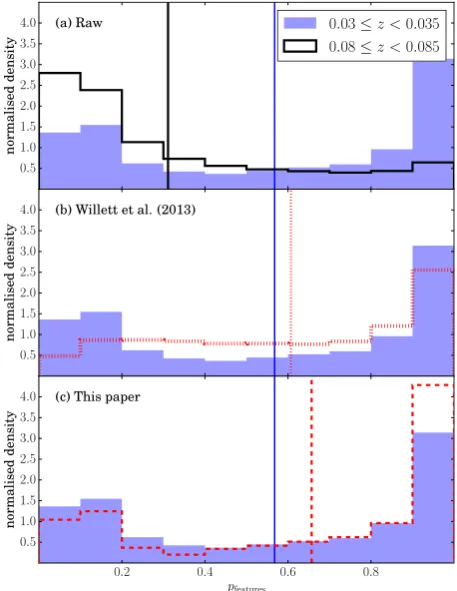
The effect of redshift bias is shown in Fig.3a, where the answer to the ‘smooth or features’ question is compared for high- and low-redshift samples. The low-redshift range of the SDSS sample is shallow enough to argue that there should be minimal change in the overall population of galaxies (Bamford et al.2009;W13). In a luminosity-limited sample, the level of completeness should also be the same at all redshifts, meaning that the overall populations of the high- and low-redshift samples should be equivalent. However, Fig.3a shows that the higher redshift vote fractions are dramatically skewed to lower values – generally, people are having greater difficulty in detecting the presence of features in the higher redshift images. Thus, there are fewer votes for galaxies showing ‘features’ and consequently more votes for galaxies being ‘smooth’. If one wished to compare a sample of galaxies with ‘features’ against one that is ‘smooth’ using the raw vote fractions, the number of galaxies with ‘features’ would be incomplete and the ‘smooth’ sample would be contaminated.

3.2 Previous corrections for redshift bias in GZ2

The previous debiasing procedure applied to both GZ1 and GZ2 focused on correcting the vote fractions of the galaxy samples by adjusting the mean vote fractions as a function of redshift. The method was first proposed in Bamford et al. (2009), and updated for GZ2 inW13. The method successfully adjusts the mean vote fractions for questions with two dominant answers, as can be seen from the vertical lines in Fig.3b: the mean of the debiased high-redshift sample is much closer to the mean of the low-high-redshift sample than for raw vote distributions (Fig.3a).

However, this technique has two limitations that make it unsuit-able if we want to divide a galaxy sample into different morphology subsets. The first issue is that adjustment of the mean vote frac-tion does not necessarily lead to correct adjustment of individual vote fractions. This can be seen in Fig.3b. Although the mean vote

Figure 3. Histograms of vote fractions for the ‘features’ response to the ‘smooth or features’ question in GZ2. In each of the panels, the blue filled histogram shows the raw vote distribution for a low-redshift 0.03≤z < 0.035 slice of theluminosity-limited sample. The unfilled histograms show the equivalent distribution for a higher redshift 0.08< z≤0.085 sample. The vertical lines show the mean vote fractions.

fraction for the high-redshift sample has been correctly adjusted to approximately match the low-redshift sample, the overall distribu-tion does not. There is an excess of debiased votes in the middle of the distribution, and fewer votes for the tails of the distribution atp≈0 andp≈1. This effect is important if we wish to divide our sample into different subsets by morphological type. As the shape of the histograms is not consistent with redshift, the fraction of galaxies withpfeaturesgreater than a given threshold can also vary

with redshift.

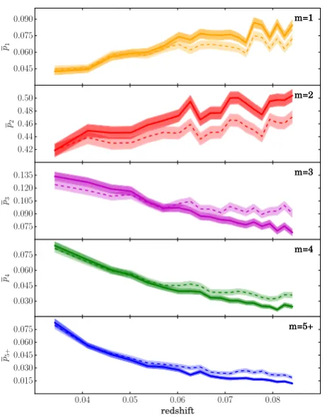
As described in Section 2.3, GZ2 utilizes multiple answered ques-tions to obtain more detailed classificaques-tions than GZ1. In cases where the votes are split between multiple categories, the debias-ing method fromW13 does not always adjust the vote fractions correctly. We show this effect for the ‘spiral arm number’ question (T10 of Fig.2), in Fig.4. A sample of ‘secure’ spiral galaxies with

pfeatures×pnot edge-on×pspiral>0.5 is selected, (with the vote

frac-tions corresponding to the debiased values fromW13), and the mean vote fractions with respect to redshift for each of the arm number responses are plotted. A clear trend inparm numberis observed: the

mean vote fractions vary systematically with redshift, even after the W13correction has been applied. For this question, the answers with more spiral arms (3, 4, or 5+spiral arms) are the ‘harder to see’ features meaning that there are fewer votes for these categories at higher redshift, which instead increase the 1 and 2 arm vote frac-tions. The 3, 4 and 5+spiral arm samples of spiral galaxies therefore suffer from incompleteness. This is of particular importance in this case for two reasons. First, as this is a ‘fourth order’ question, as

at University of Nottingham on January 5, 2017

http://mnras.oxfordjournals.org/

Figure 4. Mean vote fractions for each of the arm number responses to the ‘arm number’ question (T10 in Fig.2. The sample consists of galaxies from theluminosity-limited sample, withpfeatures×pnot edge-on×pspiral> 0.5 (with vote fractions taken from theW13debiased catalogue). The solid lines show the mean arm number vote fractions obtained using the raw vote classifications, and the dashed lines indicate the same quantity obtained using theW13debiased values. The shaded regions indicate the 1σerror on the mean.

can be seen in Fig.2, then the sample size is limited, as three ques-tions must have been answered ‘correctly’ previously for a galaxy to be classified as spiral. Secondly, the 3, 4 and 5+arm responses have low mean vote fractions overall, of0.1. Thus, the number statistics for these categories are very low, meaning they will suffer from high levels of noise. Correspondingly, the 1 and 2 armed spiral samples would suffer from contamination from galaxies that should have been classified as 3, 4 or 5+armed.

3.3 A new method for removing redshift bias

Given the limitations described in Section 3.2, we attempt to con-struct a new method of debiasing the GZ2 data more effectively. When considering a question further down the question tree with low number statistics, such as the spiral arm question, we prefer to use a thresholding technique rather than using the weighted vote fractions (see Section 2.3 for a descriptions of both methods). Using the arm number question as an example, the ‘2 spiral arms’ response dominates the overall vote fractions, making up∼60 per cent of the votes, as can be seen in Fig.4. The rarer responses of 3, 4 or 5+arms have much lower number statistics overall, with only∼10 per cent of the votes. The mean values can therefore be affected by the noise in the dominant category, which will be much larger than the noise for the rarer category. We therefore divide our galaxy sample into different sub-samples when comparing galaxies by spiral arm number.

Unlike the debiasing method inW13, our new method aims to make the vote distributions themselves as consistent as possible rather than purely aiming for consistency in the mean vote fraction values. As each galaxy is classified by 40 or more volunteers (W13), we have enough data to model the evolution of the vote distributions as a function of redshift. Different classifiers will have different sen-sitivity for picking out the most detailed features. Thus, as samples at higher redshift are considered, and hence with poorer image qual-ity, we expect the vote fraction distributions to also evolve as some classifiers become less able to see the most detailed features. We aim to account for this bias by modelling the vote fraction distri-butions as a function of redshift, and correcting the higher redshift vote distributions to be as similar as possible to equivalent vote distributions at low redshift.

We first define samples of galaxies for each of the questions in turn. The sample is then binned in terms of the intrinsic galaxy properties of size and luminosity, and each of these bins is divided into redshift slices. We then attempt to model the vote distributions for each of the bins with respect to redshift, and thus match their distributions to those at low redshift. This means that if a vote fraction threshold is applied, the fraction of galaxies with a given feature remains constant: at each redshift, the sample is composed of the galaxies that are most likely to have that particular feature.

It must be noted that such a method could still be limited by small-number statistics, which is particularly common at higher redshifts. In the case that a feature’s vote fraction drops to 0, we cannot ‘add’ votes for a feature – it is only possible to debias the galaxies with

p>0, where there is evidence for a feature being present. This remains a problem for the categories where the vote fractions are lowest, such as in the responses to the odd feature question (T06 in Fig.2).

3.3.1 Sample selection for each question

As GZ2 morphologies are classified with a decision tree (see Section 2.3), not all of the questions were answered by each of the volunteers for a given galaxy. Answering the spiral arm number question is not appropriate for all of the galaxies in the sample: if a galaxy has no spiral features, yet a volunteer answered the spiral arm question, that galaxy would contribute ‘noise’ to the answers to that question. To avoid ‘noise’ introduced by incorrectly classified galaxies, clean galaxy samples are defined withp>0.5. For the first question, this corresponds to all of the galaxies, as each classifier answered that particular question for each galaxy. However, when questions further down the tree are considered, this is not the case. The equivalent p> 0.5 for the spiral arm question would only include the galaxies withpfeatures×pnotedge-on×pspiral>0.5.

For each of the questions in turn, we define a sample of galaxies with which we will apply the new debiasing procedure. These sam-ples are defined using a cut ofp>0.5 (corresponding topfeatures× pnotedge-on×pspiral >0.5 for the spiral arm question for example).

A further cut ofN≥5 (whereNis the number of classifications) is also imposed to ensure that each galaxy has been classified by a significant number of people to reduce the effects of Poisson noise. In this case, the vote fractions must be the debiased vote values, to ensure each sample is as complete as possible (see Section 3.1) as we look at each question. The order in which the questions are debiased is important: to define a complete sample of galaxies to be used for the debiasing of a particular question, all questions further up the question tree must have been debiased beforehand.

at University of Nottingham on January 5, 2017

http://mnras.oxfordjournals.org/

Figure 5. Voronoi bins for the more than 4 arms (A4) answer to the spi-ral arm number question (T10). The sample is defined using the method described in Section 3.3.2, and binned in terms of log (R50) andMr. Dif-ferent bins are defined with difDif-ferent colours. Each Voronoi bin is further subdivided into several redshift bins.

3.3.2 Binning the data

It is expected that the ability to discern the presence of a particu-lar feature will depend on intrinsic galaxy properties. For example, larger, brighter galaxies may be easier to classify over a wider redshift range. Conversely, fainter galaxies may show stronger fea-tures, as both overall galaxy morphology (Maller2008; Bamford et al.2009) and spiral arm morphology (Kendall, Clarke & Ken-nicutt2015) have stellar mass dependences. To account for these possible variations, we bin the data in terms ofMrand log (R50) for

each answer in turn. We use thevoronoi_2d_binning pack-age from Cappellari & Copin (2003), to ensure that the bins will have an approximately equal number of galaxies. Fig.5shows an example of the Voronoi binning for the 5+arms response to the arm number question. When Voronoi binning the data for each of the answers, only theNgalgalaxies withp>0 are included, meaning

that the ‘signal’ of galaxies is evened out over all of the Voronoi bins. We aim to have∼30 Voronoi bins for each of the questions, so the desired number of galaxies in each bin is given byNgal/30.

After Voronoi binning the data in terms of their intrinsic proper-ties of size and brightness, we further divide each bin into redshift bins, to allow us to study how the vote distributions change with redshift. Each redshift bin is constrained to contain≥50 galaxies. This binned data is used for the debiasing methods described in the next section.

3.3.3 Modelling redshift bias

For each of the possible responses to each question, a method is applied to correct for the redshift bias in the sample, aiming to make the vote distributions for each answer consistent with redshift. The two methods that we employ to achieve this are described below.

The first method we utilize to remove redshift bias simply matches the shapes of the histograms on a bin-by-bin basis. The cumulative distribution for the lowest redshift sample in a given

Figure 6. An example of vote distributions for an example Voronoi bin for the ‘features or disc’ answer to the ‘smooth or features’ question. Each of the galaxies in the high-redshift bin (red dashed line) is matched to its closest equivalent low-redshift galaxy (blue solid line) in terms of cumulative fraction. The dotted lines indicate the ‘matched’ values for an example galaxy with log (p)≈ −0.8, and an equivalent low-redshift value of log (p)≈ −0.2 (corresponding topraw=0.18 andpdebiased=0.65). We plot log (p) on thex-axis rather thanpto make the two distributions more easily discernable.

Voronoi bin is used as a reference for how the shape of the his-togram would look if it were viewed at low redshift. An example of this method is shown in Fig.6, in which the ‘features or disc’ answer to the ‘smooth or features’ question is considered. For both the low-redshift bin and the high-redshift bin, the vote fractions are ranked in order of low to high. Each of the galaxies in the high-redshift bin is then matched to its low high-redshift equivalent by finding the galaxy with the closest cumulative fraction in the low-redshift bin. An example of this technique is shown by the vertical lines of Fig.6. In this case, a galaxy with cumulative fraction of≈0.8 in the high-redshift bin haspfeatures≈0.18. A galaxy at the same

cumulative fraction in the low-redshift bin haspfeatures ≈0.65, so

this is the debiased value assigned to that galaxy. This is repeated for each galaxy and for each of the high-redshift bins in turn. Ap-plying a vote fraction threshold for a given response gives the same fraction of the population above that threshold in all of the redshift bins, with the galaxies most likely to have a feature making up the population of galaxies above that threshold.

The main strength of this method is that any vote distribution can be modelled in this way, irrespective of the overall shape. How-ever, a potential weakness is that noise can be introduced due to the discretization of the data. To limit this issue, each redshift bin has a ‘good’ signal of≥50 galaxies. This effectively ‘blurs’ any trends with redshift, and can actually lead to an overcorrection of vote fractions, which can be seen in Fig.3c. Although the overall histogram shape is well matched when a slice at 0.08≤z <0.085 is considered, we see too many galaxies withp≈1 compared to the low-redshift data. This issue is purely caused by the discretization of the individual bins: although the trends can be modelled overall, any trends within individual bins cannot. If there is a redshift trend

withina bin, then the fraction of galaxies with the more difficult

at University of Nottingham on January 5, 2017

http://mnras.oxfordjournals.org/

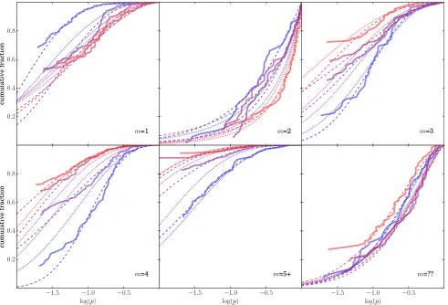
Figure 7. An example of a single Voronoi bin fit for thearm numberquestion. The red line indicates the highest redshift bin, and the blue line indicates the lowest redshift bin. The solid lines indicate the rawphistograms, and the dashed lines show the best-fitting function to each of them. The dotted lines show the corresponding approximation from the continuous fit to thekandcvalues.

to see features will preferentially reside in the lower redshift ends of the bins. This effect leads to an overestimate of the number of galaxies with the more difficult to see features. Fig.8a shows the debiased trends of the ‘features or disc’ question, which was debi-ased using the ‘bin-by-bin’ method, which shows that the method slightly overcorrects the redshift trend in the number of galaxies classified withpfeatures>0.5.

One potential solution would be to bin the data more finely. However, there is no ‘ideal’ solution to this problem, as fewer galaxies in each bin would mean that the redshift range that each bin occupies is smaller, but the noise in each of the bins is larger.

To attempt to remove the discrete nature of the correction in the ‘bin-by-bin’ method, we use an alternative method that models the vote distributions with analytic functions. For each of the redshift bins, we plot a cumulative histogram of log (p) against the cumu-lative fraction. Examples of some of these cumucumu-lative histograms are plotted as the solid lines in Fig.7. It can be seen that there is a clear evolution in the distributions with redshift. This effect is most prominent in the 4 and 5+arms responses, where the distributions shift so that there are fewer galaxies with higher vote fractions. To correct for this bias, each of the cumulative histograms can be fitted to an analytic function, and the parameters of the function modelled in terms of redshift (z), galaxy size (R50) and intrinsic brightness

(Mr). After much experimentation, a function of the following form

is used to model the cumulative distributions:

f(p)=ekpc, (1)

wherekandcare variables fit to each of the curves. Best-fittingk

andcvalues are found for each of the bins, indicated by the dashed lines in Fig.7. When fitting, the cumulative histogram is sampled evenly in log (p) to avoid the fit being weighted to the steepest parts of the curves.

After findingkandcfor each of the bins, we attempt to quantify how these parameters change with respect toMr, log (R50) andz. A

2σclipping is applied to all of thekandcvalues to remove any fits where discrepantkorcvalues have been found. The data are then fitted using a continuous function of the following form:

Afit(Mr, R50, z)=A0+AM(fM(−Mr))

+AR(fR(log(R50)))+Az(fz(z)), (2)

whereAcorresponds to eitherkorcandfM,fRandfzare functions

that can be either logarithmic (logx), linear (x) or exponential (ex_).

The valuesA0,AM,ARand Az are constants that parametrize the

shape of the fit with respect to each of the terms. When fitting the data,Mr, log (R50) andzcorrespond to their respective mean values

calculated using all of the galaxies in that bin. The best combination of functions is chosen by calculatingA0,AM,ARandAz for each

combination offM,fR andfz, and selecting the function that has

the lowest squared residuals. We then clip any values with a>2σ residual to this fit and re-fit the data to find a final functional form forkandcwith respect toMr,R50 andz. The resulting modelled

cumulative histograms for the spiral arm number question are shown by the dotted lines of Fig.7. Limits are also applied tokandcto

at University of Nottingham on January 5, 2017

http://mnras.oxfordjournals.org/

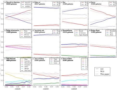
Figure 8. Number of galaxies withp>0.5 for each of the questions debiased using the method described in Section 3.3. The solid lines indicate the raw vote fractions and the dashed lines indicate the debiased vote fractions. The dotted lines indicate the same fractions using theW13debiasing method. The total sample here is composed of galaxies in theluminosity-limited samplewithp>0.5 (as described in Section 3.3.1).

avoid unphysical fits at extreme values ofMR,R50andz, set by the

upper and lower limits of all of the fitkandcvalues within the 2σ clipping.

After finding a functional form forkandcwith respect toMr,

log (R50) andz, each of the galaxies in the sample is debiased to

find its equivalent value at low redshift. To do this for an individual galaxy, a cumulative histogram is estimated usingkfit(Mr,R50,z)

andcfit(Mr,R50,z), whereMr,R50andzare the properties for that

particular galaxy, giving the cumulative fraction for a galaxy’s raw vote fraction. The equivalent cumulative histogram atz=0.03 (the low-redshift limit of ourluminosity-limited sample) is also found, usingkfit(Mr,R50, 0.03) andcfit(Mr,R50, 0.03). The vote fraction

for the corresponding cumulative fraction is read off from the low redshift cumulative histogram in a similar way as in the ‘bin-by-bin’ method, this time using the fitted curves rather than the raw histograms. This is repeated for each of the galaxies in the sample to generate a set of debiased values for thefull sampleof galaxies.

As mentioned previously, function fitting avoids issues related to the discretization of the data. However, it does introduce its own biases, as an assumption is made that the cumulative histograms can all be well-fitted by a particular set of continuous functions. This may not always be the case, so we must consider which of the above methods does the best overall job of removing redshift bias. To do

this, the distributions of votes for a low-redshift reference sample are compared to the distributions of higher redshift bins. Using the

luminosity-limited sample, which is free from redshift bias across allMr−R50 bins, a reference sample with 0.03≤z < 0.035 is

defined. The rest of theluminosity-limited sampleis then split into 10 redshift slices, and the total square residual of the vote fractions from both of the debiased methods are calculated with respect to the raw vote distributions of the reference sample. The method with the lowest total square residual is used to compute the final debiased values.

3.3.4 Results from the new debiasing method

As described in Section 3.3, the new method aims to keep the fraction of galaxies above a given threshold constant with redshift, rather than simply correcting the mean vote fractions with redshift, as shown in Fig. 3c. To test how successful the new debiasing method is at defining populations of galaxies above a given thresh-old with redshift, the fraction of galaxies withp>0.5 for each of the questions is plotted in Fig.8. It can be seen that in most cases, the new debiasing method does keep the fraction of the population withp>0.5 constant with redshift, as expected. This effect is most

at University of Nottingham on January 5, 2017

http://mnras.oxfordjournals.org/

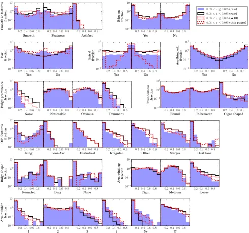
Figure 9. Vote distribution histograms for each of the answers in the GZ2 question tree. The blue filled histogram shows the distribution for galaxies with 0.03< z≤0.035, which should have minimal redshift-dependent bias. The black solid, red dotted and red dashed histograms show the distribution of galaxies at 0.08< z≤0.085 using the raw,W13debiased, and debiased data from this paper, respectively. All samples use only galaxies withp>0.5 (as described in Section 3.3.1) from theluminosity-limited sample.

evident when looking at the ‘spiral’ question (T03 in Fig.2), in Fig.8d. It can be seen that the original debiasing method does not adequately remove redshift bias, with fewer galaxies exhibiting spi-ral structure at higher redshift. However, our new method does keep this fraction approximately constant with redshift, which means the spiral sample will be more complete if we wish to use a thresholding technique to define a sample of galaxies with spiral structure.

Fig.8only shows the specific example of the threshold ofp>0.5. This does not give any insight into the overall vote fraction distri-bution, which can vary with redshift as shown in Fig.3. Therefore, overall distributions are compared for two redshift slices in Fig.9. It can be seen that this new method does not always ‘match’ the low-and high-redshift samples exactly, an effect that is most obvious in the ‘spiral’ question. Rather than getting an excess of votes towards

the middle of the distribution, excesses are more generally seen at the tails of the distributions atp≈0 andp≈1. This is because our method preferentially matches thep≈1 end of the distribution. As can be seen by the ‘spiral=yes’ response in Fig.9, the top ends of the distributions are usually correctly matched; the scarcity of votes for the intermediate values ofpare caused by the excess of galaxies withp=0 that cannot be corrected.

3.4 Debiased data

The data from the new debiasing method described in this Section 3.3 is available from data.galaxyzoo.org. Alongside the raw vote fractions, our new debiased vote fractions are listed, as well as a gz2_class and flags for ‘securely’ detected spiral or elliptical

at University of Nottingham on January 5, 2017

http://mnras.oxfordjournals.org/

Table 1. Example portion of the output table from the new debiasing method, showing the results from the ‘smooth or features question (T11)’, and, ‘smooth answer (A0)’. The full, machine-readable version of this table is available athttp://data.galaxyzoo.org.

DR7 ID RA Dec gz2_class N_class N_votes wt_count wt_fraction Debiased Flag

587732591714893851 11:56:10.32 +60:31:21.1 Sc+t 45 342 0 0 0 1

588009368545984617 09:00:20.26 +52:29:39.3 Sb+t 42 332 1 0.024 0.024 1

587732484359913515 12:13:29.27 +50:44:29.4 Ei 36 125 28 0.78 0.78 1

587741723357282317 12:25:00.47 +28:33:31.0 Sc+t 28 218 1 0.036 0.036 1

587738410866966577 10:44:20.73 +14:05:04.1 Er 43 151 33 0.767 0.767 1

587729751132209314 16:27:41.13 +40:55:37.1 Ei 48 154 41 0.861 0.861 1

587733608555216981 16:37:53.91 +36:04:22.9 Ei 39 142 25 0.649 0.649 1

587735742617616406 16:12:35.22 +29:21:54.2 Sb+t 35 282 0 0 0 1

587738574068908121 13:01:06.73 +39:50:29.3 Ei 50 158 42 0.856 0.856 1

587731870708596837 12:12:14.89 +56:10:39.1 Sb?t 43 275 8 0.194 0.194 0

galaxies (described in more detail inW13). A portion is shown in Table1to show the form and content of the data. The table includes the weighted counts and weighted fractions fromW13, with our debiased vote fractions.

4 P R O P E RT I E S O F S P I R A L G A L A X I E S W I T H R E S P E C T T O A R M N U M B E R

Despite how prevalent spiral galaxies are in the local Universe, formulating a single, complete picture as to how they form and evolve is still elusive. Spiral arms are associated with enhanced levels of gas density (e.g. Grabelsky et al.1987; Elmegreen & Elmegreen1987a; Engargiola et al.2003), star formation (Seigar & James2002; Grosbøl & Dottori2012) and dust opacity (Holw-erda et al.2005). One of the key reasons why this is the case is because spiral structure can take many varied appearances. Spiral galaxies are often classified using either their Hubble type (Hubble 1926) or an Elmegreen-type classification scheme (Elmegreen & Elmegreen1982,1987b). Using the Hubble method, spiral galaxies are assigned Hubble types depending on their bulge prominences and pitch angles. More detailed classification can be applied using the de Vaucouleurs classification scheme (de Vaucouleurs1959, 1963), where the presence of more detailed structure such as dif-fuse, irregular spiral arms and rings can also be morphologically assigned. However, the Hubble-type classification scheme and its later revisions classify spiral galaxies by their bulge prominence and their spiral arm pitch angle. These properties are weakly related (Kennicutt1981; Seigar & James1998): spiral arm tightness has been shown to be more strongly correlated with bulge total mass (Seigar et al.2008; Berrier et al.2013; Davis et al.2015), rather than bulge-to-disc ratio. The Elmegreen-type classifications scheme instead divides galaxies into different types depending on the spi-ral arm structure itself, rather than any properties related to the galactic bulge. This scheme generally classifies galaxies as one of three types: grand design, multiple-armed or flocculent. Grand de-sign spiral structure is associated with two symmetric spiral arms, whereas multiple-armed structure is associated with more than two spiral arms and flocculent galaxies have many, shorter, less well-defined arms. The distinct advantage to classifying spiral galaxies in this way is that contrasting physical mechanisms are thought to play a role in the formation of these two different types of spiral structure.

Grand design spiral structure was initially thought to be due to the presence of a density wave in a galaxy’s disc (Lindblad1963; Lin & Shu1964), in which gas is ‘shocked’ into forming stars in regions of high density in the disc. However, this mechanism is no longer favoured, as there is no evidence for the enhancement of star

formation in grand design spiral galaxies compared to many-armed spiral galaxies of the same stellar mass (Elmegreen & Elmegreen 1986; Dobbs & Pringle2009), or any evidence for enhancement in star formation in the individual arms of such galaxies (Foyle et al. 2011; Choi et al. 2015). Instead, it is thought that grand design spiral structure may actually occur as a result of strong bars in galaxy discs or tidal interactions (Kormendy & Norman 1979). Early observational evidence supports the theory that grand design structure can be induced via interactions, with two-armed structure being favoured over many-armed structure in high-density environments (Elmegreen & Elmegreen1982,1987b; Ann2014), and simulations showing that galaxy–galaxy interactions can lead to grand design spiral structure in galaxy discs like that seen in the local Universe (Dobbs et al.2010; Semczuk & Lokas2015).

Unlike two-armed spiral structure, many-armed spiral structure arises readily in simulations without the requirement for a trigger from either a bar instability or a tidal interaction (James & Sellwood 1978; Sellwood & Carlberg1984). Such structures require a cooling of the gas in the disc to be sustained for long periods of time (Carlberg & Freedman1985). More recent simulations, taking the disc gravity into account, have shown that ‘flocculent’ structure may actually be a transient feature of spiral galaxies, with spiral arms continually being made and destroyed (Bottema2003; Baba et al.2009; Grand, Kawata & Cropper2012; Baba, Saitoh & Wada 2013; D’Onghia, Vogelsberger & Hernquist2013), rather than a long-lasting persistent structure.

Despite the recent advances in the simulations of these disc galax-ies, the picture as to how all of the processes shape spiral galaxies still remains unclear. Grand design spiral galaxies can still reside in low-density environments without the presence of bars (Elmegreen & Elmegreen1982), meaning that they are not purely driven by these processes as described in Kormendy & Norman (1979). Ad-ditionally, the time-scales of the persistence of spiral structure is still unclear, particularly as older stellar populations viewed in the in-frared show very different structure to the young stellar populations viewed at optical wavelengths (Block & Wainscoat 1991; Block et al.1994; Thornley1996). Most recent work on spiral structure have also mainly been focused on simulations of spiral structure. Putting observational constraints requires the visual inspection of the spiral arm structure in galaxy discs, so have been restricted to relatively small samples of order2000 galaxies [e.g. Elmegreen & Elmegreen (1982,1989); Ann & Lee (2013)]. We use the GZ2 vote classifications to compare the overall demographics of spi-ral structure in a much larger sample of SDSS galaxies, defining galaxy samples which are complete in both luminosity and stel-lar mass (see Section 2 for descriptions of how these samples are defined).

at University of Nottingham on January 5, 2017

http://mnras.oxfordjournals.org/

4.1 Spiral arms in Galaxy Zoo

In order to study how spiral properties vary, visual inspection of the number of arms in a spiral galaxy disc is required. Such classifica-tions are provided by question T10 of the GZ2 question tree (see Fig.2). This question has six possible responses. In this case, the responses will be referred to asm-values, and can take the value of either 1, 2, 3, 4, 5+or ‘can’t tell’.

In order to compare different spiral galaxies, a secure sample of spirals must first be defined. The sample is defined by selecting galaxies withpfeatures×pnotedge-on ×pspiral >0.5. A further cut is

also imposed where only galaxies withNspiral−Ncant tell≥5 are

selected, meaning thatat least five peopleclassified the spiral arm number of each of the spiral galaxies, reducing the effects of noise due to low numbers of classifications. The population of galaxies selected in this way from thefull samplewill hereafter be referred to as thespiral sample. The samples defined using these same cuts from theluminosity-limited sampleandstellar mass-limited sample

are referred to as theluminosity-limited spiral sampleandstellar mass-limited spiral sample.

Each galaxy is then assigned a specific spiral arm numberm, of either 1, 2, 3, 4 or 5+arms, depending on which response has the highest debiased vote fraction (excluding thecan’t tellresponse). Thedebiasedvote fractions for each of the arm number responses are hereafter referred to aspm, wheremis either 1, 2, 3, 4 or 5+.

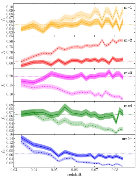
The debiasing procedure applied to this question has shifted the vote fractions for the multiple-armed (m=3, 4, 5+) answers up-wards overall, as can be seen in Fig. 10. This has the effect of making each of these samples more complete with redshift, and increasing their respective overall vote fractions. However, in the

m= 5+arms case, the sample is still somewhat incomplete, as the overall fraction of galaxies that are assigned to this category decreases with redshift. The vote fractions form=5+fall to 0 far more quickly with redshift than any of the other categories, as can be seen from the dashed line in the bottom panel of Fig.10, making the modelling of this redshift bias difficult. Despite this, the fraction of galaxies that make up them=5+category are still significantly improved compared to the sample sizes that would be defined using either the raw vote fractions or theW13debiased vote fractions, as can be seen in from theNandfcolumns of Table2. Examples of some securely classified spiral galaxies are shown in Fig.11, where each galaxy has a dominant vote fraction ofpm>0.8. The samples

of galaxies assigned to each of the differentm-values are referred to as thearm number samples.

Figure 10. Fraction of galaxies in theluminosity-limited spiral sample

classified as having 1, 2, 3, 4, or 5+spiral arms as a function of redshift. The solid lines indicate the fractions from the debiased values in this paper, and the dashed lines indicate the same fractions using the raw vote fractions. Errors are calculated using the method described in Cameron (2011). The horizontal dotted lines show the mean fractions using the debiased values averaged over all of the bins.

The main result of this debiasing is that galaxies with low vote fractions for the armed answers are included in the many-armed categories when they were not before. As a consequence, the population ofm=2 galaxies is less contaminated by galaxies that actually have 3, 4 or 5+spiral arms. This effect is illustrated in Fig.12, where a selection of spiral galaxies with 0.5<pm≤0.6 are

shown. It can be seen that them=4 andm=5+spiral samples at higher redshift include spiral galaxies that initially had much lower overall vote fractions. As an example, if one were to use the raw

Table 2. Overall properties of galaxy populations with different numbers of spiral arms. The number of galaxies with 1, 2, 3, 4 and 5+arms are shown for both theluminosity-limitedandstellar mass-limited spiral samples. Mean stellar masses, colours and local densities are shown for each of the populations, with 1σstandard deviations indicated in parentheses. Errors on the mean (σ/√Ndebiased) are all of order<0.01.

m Nraw fraw NW13 fW13 Ndebiased fdebiased M∗(log(M/M)) g−i (Mpc−2)

Luminosity-limited 12 554 1.00 14297 1.00 17 957 1.00 10.62 (0.25) 0.82 (0.17) −0.24 (0.56)

1 563 0.04 670 0.05 926 0.05 10.63 (0.28) 0.83 (0.19) −0.25 (0.54)

2 9044 0.72 10073 0.7 11 157 0.62 10.63 (0.24) 0.86 (0.17) −0.21 (0.57)

3 1778 0.14 2158 0.15 3552 0.2 10.59 (0.26) 0.75 (0.15) −0.28 (0.53)

4 615 0.05 751 0.05 1162 0.06 10.60 (0.26) 0.74 (0.15) −0.30 (0.51)

5+ 554 0.04 645 0.05 1160 0.06 10.65 (0.27) 0.75 (0.16) −0.30 (0.53)

Stellar mass-limited 6683 1.00 7226 1.00 9413 1.00 10.81 (0.16) 0.91 (0.14) −0.18 (0.57)

1 290 0.04 331 0.05 500 0.05 10.84 (0.16) 0.94 (0.14) −0.19 (0.53)

2 4852 0.73 5191 0.72 6059 0.64 10.80 (0.15) 0.94 (0.13) −0.15 (0.59)

3 886 0.13 991 0.14 1654 0.18 10.82 (0.16) 0.83 (0.12) −0.23 (0.53)

4 335 0.05 366 0.05 565 0.06 10.82 (0.16) 0.82 (0.12) −0.25 (0.53)

5+ 320 0.05 347 0.05 635 0.07 10.85 (0.18) 0.82 (0.13) −0.26 (0.53)

at University of Nottingham on January 5, 2017

http://mnras.oxfordjournals.org/

Figure 11. Galaxies classified in each of the arm number categories (m=1, 2, 3, 4 or 5+) for the stellar mass range 10.0<logM_∗/M _≤11.0. All of the galaxies are taken from theluminosity-limited spiral sample. Each galaxy has a debiased modal vote fractionpm>0.8.

vote fractions to select ‘secure’ galaxy samples withpm>0.5, then

the galaxy in Fig.12y would be unclassified, as its highest value of

pmwould only be 0.27 (which is actually for them=4 response).

Using our debiased values, it has a modal value ofpm=0.55 for

them=5+armed response, so would be in them=5+sample. Even in the case of the less secure samples of Fig.12, the galaxies classified asm=4 orm=5+clearly have more spiral arms than those in them=2 category.

4.2 Comparing galaxy populations

Having defined the samples of spiral galaxies in Section 4.1, the demographics of the different galaxy populations separated by spiral arm number can be compared. For reference, mean stellar mass (M_∗), colour (g−i) and local densities [, as described in Baldry et al. (2006); Bamford et al. (2009)] are tabulated in the final three columns of Table2.

4.2.1 Comparison of sample sizes

Spiral arm multiplicity does not map exactly to a specific Elmegreen-type for two reasons. First, the arm number itself does not give any indication of the prominence of spiral arms, so cannot be used to distinguish between a galaxy with many well-defined arms and one with more flocculent spiral structure, which are usu-ally defined differently (Elmegreen & Elmegreen1982, 1987b). The second issue is that arm structure may not necessarily be con-sistent at all radii (Grosbøl, Patsis & Pompei2004) or at all wave-lengths (Block & Wainscoat1991; Block et al.1994; Thornley1996) within a galaxy disc, meaning that assigning a singlem-value of arm number may not give a complete picture of the overall spiral arm structure. The most ‘easy-to-map’ categories may therefore be to compare them=2 population with the galaxies classified as grand design, as grand design structure is usually associated with two well-defined arms across the entire disc (Elmegreen & Elmegreen

at University of Nottingham on January 5, 2017

http://mnras.oxfordjournals.org/

Figure 12. Galaxies classified in each of the arm number categories (m=1, 2, 3, 4 or 5+) for the stellar mass range 10.6<logM_∗/M _≤11.0. All of the galaxies are taken from theluminosity-limited spiral sample. Each of the galaxies is assigned to an arm number category by its modalpmvalue. All of the modalpm-values lie in the range 0.5<pm≤0.6.

1982). In theluminosity-limited spiral sample, 62.1±0.4 per cent of the galaxies show two-armed spiral structure. This result is con-sistent with optical visual classifications (Elmegreen & Elmegreen 1982) and infrared classifications (Grosbøl et al.2004), which sug-gest that∼60 per cent of local spiral galaxies exhibit grand design spiral structure.

4.2.2 Stellar mass

Galaxy stellar mass is known to correlate with galaxy morphology (Bamford et al.2009; Kelvin et al.2014b), and spiral galaxy Hubble type (Mu˜noz-Mateos et al.2015). It has been demonstrated that the

centralmass of spiral galaxies can play a role in the type of spiral structure exhibited in spiral galaxies. In particular, the pitch angle of spiral arms is related to both the star-formation rate in spiral galaxies (Seigar2005), and the central mass concentration of the

spiral galaxies (Seigar et al.2006,2014). Total galaxy stellar mass has also been found to correlate with observed spiral structure, with the strength of them= 2 mode in spiral galaxies being stronger in galaxies with greater physical size (Elmegreen & Elmegreen 1987b) and stellar mass (Kendall et al.2015). In this section we will investigate whether the total galaxy stellar mass has any influence on the number of spiral arms in spiral galaxies.

The method for measuring stellar mass, described in Baldry et al. (2006), uses theu− rand Mrvalues from the SDSS. To avoid

contamination of galaxies with uncertain stellar masses due to poor flux detection in these bands, only galaxies withF/δF>5 (where

Fis the flux error in a given band, andδFis the equivalent error on the flux) in both u and r are included in this analysis. The distributions of stellar mass for each of thearm number samplesare shown in Fig.13a. The overall distributions for each of the galaxy samples show that there is little evidence for a dependence of spiral

at University of Nottingham on January 5, 2017

http://mnras.oxfordjournals.org/

Figure 13. Left: distributions of stellar mass for theluminosity-limited spiral sample. The solid lines indicate the distributions for each of thearm number samplesfor each of arm numbers. The grey filled histograms show the equivalent distribution for all of the spiral galaxies for reference. The black dotted line indicates the stellar mass values above which the sample is complete in stellar mass. Right: fraction of thestellar mass-limited spiral sampleclassified as having each spiral arm number, in 20 bins of stellar mass. The shaded regions indicate the 1σerror calculated using the method described in Cameron (2011).

arm number with respect to host galaxy stellar mass; each of the samples contains galaxies across the entire range of stellar mass from 10.0log(M_∗/M)11.5. A slight excess of low-stellar mass galaxies is found in them=3 andm=4 samples, as well as an excess of high-stellar mass spiral galaxies for them=5+ sample.

The distributions of Fig.13a show the distributions from the

luminosity-limited spiral sample, so are therefore incomplete for galaxies with lower stellar masses (see Section 2.1) thanM_∗ 1010.6_M

, indicated by the black dotted line. As we shall see in Section 4.2.4, lower mass galaxies are bluer, and hence more lu-minous for a given stellar mass. They are thus overrepresented at low masses in a luminosity-limited sample. To look for trends in terms of stellar mass, the overall fraction of thestellar mass-limited spiral sampleis shown in Fig.13b. Now, it can be seen that there do appear to be some trends between spiral arm number and host galaxy stellar mass. A significant increase in the fraction of galax-ies with 5+spiral arms is observed from the overall mean value of 0.068± 0.002 to 0.15±0.02 for the highest stellar mass bin of log(M∗/M)=11.2±0.1. The m= 3 and m= 4 samples hint at similar, but much weaker trends. Conversely, the fraction of galaxies with two spiral arms decreases from 0.642± 0.004 for the total population to 0.53±0.02 in the highest stellar mass bin.

One possibility why higher mass spirals may exhibit more spiral arms is that this could purely be an effect from the visual classi-fications. It has already been identified that the many-armed spiral features are the most difficult to detect, so may be more easily identifiable in the largest, brightest spiral galaxies. Spiral arms are

already known to have greater amplitudes (i.e. be more prominent) in galaxies with larger stellar masses (Kendall et al.2015). It has already been demonstrated in Section 3.3.4 that them=5+ sam-ple is the most incomsam-plete of the samsam-ples divided by spiral arm number. Thus, galaxies with greater stellar mass, that are therefore larger and brighter, may be preferentially put in this category, even after debiasing.

Another interesting scenario may be that the population of galax-ies with the highest stellar mass are a population of unquenched spiral galaxies as in Ogle et al. (2016). Such galaxies still have their discs intact, so have no signatures of tidal interactions. As galaxy– galaxy interactions have been linked to both the inducement of two-armed spiral structure (Dobbs et al.2010; Semczuk & Lokas 2015), and the depletion of gas and therefore quenching (Di Matteo et al.2007; Li et al.2008), then one may conclude that the discs of these galaxies have not been disturbed. A possible explanation for this is that lower mass galaxies are more susceptible to environ-ment effects (Bamford et al.2009), so these discs are still forming stars in the transient way with multiple spiral arms, as described in Section 4.

4.2.3 Local environment

It is already well established that there is a clear dependence of the type of spiral structure that galaxies exhibit with respect to their local environment. Observational evidence from comparison of vi-sually classified galaxies has found that grand design galaxies are more prominent in high-density group environments and in binary systems where a close companion galaxy is present (Elmegreen &

at University of Nottingham on January 5, 2017

http://mnras.oxfordjournals.org/

Figure 14. Left: distributions of local density () for thestellar mass-limited spiral sample. The solid lines indicate the distributions for each of thearm number samplesfor each of arm numbers. The grey filled histograms show the equivalent distribution for all of the spiral galaxies for reference. Right: fraction of thestellar mass-limited spiral sampleclassified as having each spiral arm number, in 20 bins of. The shaded regions indicate the 1σerror calculated using the method described in Cameron (2011).

Elmegreen1982,1987b; Seigar, Chorney & James2003; Elmegreen et al.2011). These results suggest that a mechanism is responsible for the transformation of spiral structure as galaxies enter the high-est density environments, with a plausible explanation being that two-armed spiral structure is the result of a recent gravitational in-teraction.N-body modelling of galaxies has shown that two-armed spiral structure can occur as a result of galaxy–galaxy interactions (Sundelius et al.1987; Dobbs et al.2010). However, the time-scales of the persistence of such structures are thought to be relatively short-lived (Oh et al.2008; Dobbs et al.2010), meaning that an en-hancement in the fraction of grand design galaxies is only observed in the highest density environments where interactions can happen on a frequent enough basis to sustain such structures (Elmegreen & Elmegreen1987b).

To compare spiral arm structure as a function of environment, a mean of4and5is used as an estimate of local density, as in

Baldry et al. (2006); Bamford et al. (2009), denoted as. logis calculated as the mean of the density enclosed within the projected distance to the 4th and 5th neighbour and is hence an adaptive scale that probes both large scales outside groups and local scales within groups.

The distributions of galaxy local densities for each of thearm number samples are shown in Fig. 14a. Here, the stellar mass-limited spiral sampleis used to define the total population, asM∗ and density are closely related (Baldry et al.2006), so any biases in terms of the stellar mass distributions may have an effect on the completeness of the galaxy sample in terms of environment. The distributions show a modest dependence of spiral arm number with

local density. However, as was the case for stellar mass, each of the arm number samples spans the entire range of local density defined by.

The fraction of spiral galaxies which exhibit each of the spi-ral arm numbers as a function of log are shown in Fig.14b. A clear trend is observed, with the number of two-armed spiral galax-ies increasing for the highest values of local density from 64.3± 0.5 per cent for the overall population to 75± 2 per cent for the highest density bin of log = 1.1±0.2. Conversely, all of the many-armed samples withm=3,4 or 5+all show the opposite trends, with their respective fractions decreasing with. These re-sults therefore seem to be in qualitative agreement with Elmegreen & Elmegreen (1982) and Ann (2014), in which the fraction of galax-ies displaying grand design spiral structure increases in the highest density environments. As the increase seems to be most distinct in the very highest densities, this could be indicative that two-armed spiral structure is a short-lived phase induced by galaxy–galaxy interactions, as described in Elmegreen & Elmegreen (1983). Inter-estingly, there is no clear enhancement in the fraction of galaxies with a single spiral arm at the highest densities, as found in Casteels et al. (2013). However, Casteels et al. (2013) found the most signif-icant enhancements inm=1 galaxies when galaxies have a close companion, which is not probed by our measure of environment. A more complete analysis of spiral structure with local environment, accounting for both interaction probabilities and local density will need to be considered to look for more significant trends of spiral arm structure with environment. With our large, clean samples of galaxies with measurements of arm number, we plan to take a more

at University of Nottingham on January 5, 2017

http://mnras.oxfordjournals.org/