ELEMENT METHODS
PAUL HOUSTON AND THOMAS P. WIHLER
Abstract. This article is concerned with the numerical solution of convex variational problems. More precisely, we develop an iterative minimisation technique which allows for the successive enrichment of an underlying discrete approximation space in an adaptive manner. Specifically, we outline a new approach in the context ofhp–adaptive finite element methods employed for the efficient numerical solution of linear and nonlinear second–order boundary value problems. Numerical experiments are presented which highlight the practical performance of this newhp–refinement technique for both one– and two–dimensional problems.
1. Introduction
Over the last few decades, tremendous progress has been made on both the math-ematical analysis and practical application of finite element methods to a wide range of problems of industrial importance. In particular, significant contributions have been made in the area ofa posteriorierror estimation and automatic mesh adapta-tion. For recent surveys and historical background, we refer to [2,8,15,18,30,32], and the references cited therein. Here, adaptive methods seek to automatically enrich the underlying finite element space, from which the numerical solution is sought, in order to compute efficient and reliable numerical approximations. The standard approach used within much of the literature is to simply undertake local isotropic refinement of the elements (h–refinement). However, in recent years, so-calledhp– adaptive finite element methods have been devised, whereby both local subdivision of the elements and local polynomial-degree-variation (p–refinement) are employed. These ideas date back to the work by Babuˇska and co-workers (cf. [4–7]); see also the recent books [11, 21, 28, 29], and the references cited therein. The exploitation of generalhp–refinement strategies can produce remarkably efficient methods with high algebraic or even exponential rates of convergence. Moreover, such approaches can also be combined with anisotropic refinement techniques in order to efficiently approximate problems with sharp transition features. These techniques enable the user to perform accurate and reliable computational simulations without excessive computing resources, and with the confidence that complex local features of the underlying solution are accurately captured.
Many physical processes can be modelled by locating critical points of a given (in our setting, convex) energy functional, over an admissible space of functions; a
2010Mathematics Subject Classification. 65N30.
Key words and phrases. Convex variational problems, hp–finite element methods, hp– adaptivity, quasilinear partial differential equations.
PH acknowledges the financial support of the Leverhulme Trust.
typical example includes quasilinear partial differential equations (PDEs). In this article we consider the application of adaptive finite element techniques, employ-ing a combination of hp–mesh refinement, to problems of this type. In particular, we consider a new and widely applicable paradigm for adaptive mesh generation within which we directly seek to construct the hp–finite element space in order to approximate the critical point of the underlying energy functional associated to the problem of interest. The simplest such example is the one–dimensional Poisson equation on the interval (0,1), subject to a loadf; in this case, we seek to minimise
E(u) =1/2∫1 0 u
2
xdx− ∫1
0 f udxover an appropriate solution spaceV (which naturally
incorporates the boundary conditions). The corresponding standard Galerkin finite element approximation of this problem automatically inherits the same energy min-imisation property with respect to the underlying finite element spaceVh⊂V, i.e., the finite element solution is the unique minimiser ofE(·) overVh. With this idea in mind, a natural approach is to adaptively modify the finite element spaceVhin a manner which seeks to directly decrease the energyE, i.e., denoting the new finite element solution and finite element space by u′h and Vh′, respectively, we require that E(u′h)≤E(uh). By considering an appropriately defined elementwise energy functional ˜E′κ, withκdenoting the current element in the underlying computational mesh, we devise a competitive refinement strategy which marks elements for refine-ment. More precisely, in the context of our one–dimensional example, consider an
h–refinement strategy which subdivides each element into two sub-elements. We may then compute the numerical solution to a local finite element problem posed on a local patch of elements which includes the two sub-elements. On the basis of this local reference approximation, we may then determine the predicted (elemen-tal) energy loss if the proposed refinement (i.e., a bisection of each element into two sub-elements) is undertaken. Once the predicted energy loss has been computed for all elements in the mesh, a percentage of elements with the largest predicted energy loss may be identified and subsequently refined. This idea naturally extends to the p–refinement setting, whereby, additional higher–order modes are used to locally enrich the finite element solution elementwise. With this in mind, we pro-pose a competitive hp–adaptive refinement strategy which computes the maximal predicted energy loss on each element based on comparing ap–refinement of each element (i.e., an isotropic increase of the elemental polynomial degrees by 1) with a collection of h–refinements of the same element (featuring different local poly-nomial degree distributions), which are selected so as to lead to the same increase in the number of degrees of freedom associated with the current element as the
p–enrichment, cf. [11, 12, 27, 29]. A key aspect of this algorithm is the computa-tion of a local elementwise/patchwise reference solucomputa-tion needed for the definicomputa-tion of ˜E′κ. In order to illustrate the key ideas, for the purposes of this article, we re-strict our discussion to convex optimisation problems posed on a computational domain Ω ⊂ Rd, d ≥1. However, we point out that this strategy is completely general in the sense that it can be applied to any physical problem which may be modelled as a critical point of a given energy functional E (including saddle point problems, see, e.g., [26]). In particular, one of the key advantages of our proposed approach is that it naturally facilitates the use ofhp–mesh adaptation, and indeed even anisotropic hp–mesh refinement. By considering an enrichment of the finite element space locally using any combination of isotropic/anisotropic
leads to the maximal predicted energy loss. This is in contrast to standard adap-tive techniques, whereby elements are marked for refinement according to the size of a locala posteriorierror indicator. Indeed, in this latter setting, such indicators rarely contain information concerning how the local finite element space should be enriched, but only indicate that a refinement should be performed. Thereby, alter-native numerical techniques must be devised which are capable of determining the direction of refinement (for anisotropic refinement) or the type of refinement (h– or
p–). For the latter case, such strategies include regularity estimation [14, 19, 22, 33], use ofa prioriknowledge [9, 31], and the computation of reference solutions within competitive refinement strategies [3, 11, 13, 16, 17, 23, 25, 27, 29], for example. This latter class of methods, cf. in particular [11, 12, 27, 29] and [16, 17], are very much in the spirit of the proposed competitive refinement algorithm developed in this article. Finally, we refer to [24] for an extensive review and comparison of many of thehp–adaptive refinement techniques proposed within the literature.
This article is structured as follows. In Section 2 we briefly present an abstract framework for variational problems, and consider an application to quasilinear par-tial differenpar-tial equations. Subsequently, in Section 3, thehp-version finite element discretisation of such problems is presented, and a new hp-adaptivity approach is developed in detail. The theory will be illustrated with a number of numerical experiments on linear and quasilinear boundary value problems in Section 5. Fi-nally, in Section 6 we summarise the work presented in this article and draw some conclusions.
Throughout this article, we let Lp(D), p ∈ [1,∞], be the standard Lebesgue space on some bounded domain D, with boundary ∂D, equipped with the norm
∥·∥Lp(D). Furthermore, fork∈N, we writeWk,p(D) to signify the Sobolev space of
orderk, endowed with the norm∥·∥Wk,p(D)and seminorm|·|Wk,p(D). Forp= 2 we
writeHk(D) in lieu ofWk,2(D); moreover,H1
0(D) denotes the subspace ofH1(D)
of functions with zero trace on∂D.
2. Variational Problems
In this section we outline an abstract framework for variational problems in Banach spaces, and consider an application to quasilinear boundary value problems.
2.1. Abstract Minimisation Problem. On a real reflexive Banach spaceX let us consider the minimisation problem
(2.1) min
u∈XE(u)≡umin∈X{F(u)− ⟨l, u⟩}.
Here, ⟨·,·⟩ is the duality product on X ×X′, where X′ signifies the dual space of X, and l ∈X′ is given. Furthermore, throughout this manuscript, we suppose thatF: X →Ris a continuous and strictly convex functional on X, i.e.,
F(v1+t(v2−v1))<F(v1) +t(F(v2)−F(v1)) ∀t∈[0,1]∀v1, v2∈X.
In addition, we make the assumption thatF satisfies the coercivity type condition
(2.2) F(u)− ⟨l, u⟩ →+∞ as ∥u∥X → ∞,
where ∥ · ∥X is a norm on X. Then, (2.1) possesses a unique minimiser u⋆ ∈X; see, e.g., [34, Corollary 42.14]. Furthermore, the problem of findingu⋆∈X can be written in weak form as
provided thatFhas a sufficiently regular Gˆateaux derivativeF′.
2.2. Model Problem. We now consider a specific application of the above ab-stract setting. To this end, let Ω ⊂ Rd, d ≥ 1, be an open bounded Lipschitz domain with boundary∂Ω. We consider the following quasilinear partial differen-tial equation:
−∇ ·(µ′(∇u⋆)) +g′(u⋆) =f, in Ω, u⋆= 0, on∂Ω.
(2.3)
Here, f =f(x), µ=µ(∇u), andg =g(u) are given functions, andu⋆ =u⋆(x) is the unknown analytical solution. We suppose thatf ∈Lq(Ω), for someq >1. The corresponding variational problem reads:
(2.4) min
u∈XE(u) := minu∈X ∫
Ω
{µ(∇u) +g(u)−f u}dx,
whereX =W01,p(Ω) for some suitable p >1.
With this notation, the following proposition holds.
Proposition 2.5. Letµandgfrom(2.4)be strictly convex and convex, respectively, and both continuous onRdandR, respectively. Furthermore, suppose that, for some constants C1, C2>0,p >1, andc1, c2∈Rthe lower bounds hold,
µ(ξ)≥C1|ξ|p,
(2.6)
g(η)≥c1η+c2,
(2.7)
as well as the growth conditions
µ(ξ)≤C2(1 +|ξ|p),
(2.8)
g(η)≤C2(1 +|η|p),
(2.9)
for anyξ∈Rdand anyη∈R. Then, for any givenf ∈Lq(Ω), where1/p+1/q= 1,
(2.4)has a unique solution inX =W01,p(Ω)as well as on any linear subspace ofX. Proof. Let us define
u7→F(u) := ∫
Ω
{µ(∇u) +g(u)−f u} dx.
Then, we can cast (2.4) into the abstract framework of (2.1), withl= 0 inX′. We check the conditions from Section 2.1 separately. To this end, we follow the proof presented in [34, Example 42.15].
(i) Continuity ofF: Let us consider a sequence{un} ⊂W
1,p
0 (Ω), with a limitu∈ W01,p(Ω), i.e., un → uas n → ∞. Then, with (2.8), the Nemyckii operator
ζ 7→ µ(ζ) is continuous from [Lp(Ω)]d to L1(Ω); see [35, Proposition 26.6].
Therefore,
∫Ω{µ(∇u)−µ(∇un)}dx≤ ∥µ(∇u)−µ(∇un)∥L1(Ω)→0
as n→ ∞. Similarly, using (2.9), asn→ ∞, we have that
∫Ω{g(u)−g(un)}dx →0.
(ii) Strict convexity of F: This simply follows from the strict convexity ofµ and the convexity ofg.
(iii) Coercivity: According to (2.6) and (2.7), we find that
F(u)≥C1|u|pW1,p(Ω)+
∫
Ω
{g(u)−f u}dx
≥C1|u|pW1,p(Ω)+
∫
Ω
{c1u+c2−f u}dx
≥C1|u|
p
W1,p(Ω)− |c1|∥u∥L1(Ω)+c2|Ω| −
∫Ωf udx,
where |Ω|signifies the volume of Ω. Employing the Poincar´e-Friedrich’s and H¨older’s inequalities, we arrive at
F(u)≥C∥u∥pW1,p(Ω)−(ec1+∥f∥Lq(Ω))∥u∥Lp(Ω)−ec2 ≥C∥u∥pW1,p(Ω)−(ec1+∥f∥Lq(Ω))∥u∥W1,p(Ω)−ec2,
for some constantsec1,ec2>0 depending on Ω. Therefore, it follows that
E(u) =F(u)− ⟨l, u⟩ ≡F(u)→ ∞,
with∥u∥W1,p(Ω)→ ∞. This is the coercivity condition (2.2).
The result now follows from [34, Corollary 42.14]. □
3. hp-Finite Element Discretisation
Consider now a linear subspace Xn ⊂ X with dim(Xn) = n < ∞. Then, by our previous assumptions onF, solving the finite dimensional convex optimisation problem minu∈XnE(u) for the unique minimiser u
⋆
n ∈ Xn results in an approxi-mation of u⋆ ∈X from (2.1) with u⋆
n ≈u⋆. This is the well-known Ritz method. Equivalently, in weak form, we may seeku⋆
n ∈Xn such that the Galerkin formula-tion
⟨F′(u⋆n), v⟩=⟨l, v⟩ ∀v∈Xn is satisfied; cf. [34,§42.5].
For the purposes of discretising our model problem (2.3), we will focus on an
hp–finite element approach. To this end, let us first introduce some notation: We let T = {κ} be a subdivision of the computational domain Ω into disjoint open simplices such that Ω =∪κ∈T κand denote byhκthe diameter ofκ∈ T; i.e.,hκ= diam(κ). In addition, to each elementκ∈ T we associate a polynomial degree pκ,
pκ≥1, and collect thepκ in the polynomial degree vectorp= [pκ:κ∈ T]. With this notation we define thehp–finite element spaces by
V(T,p) ={v∈H1(Ω) : v|κ∈Ppκ(κ)∀κ∈ T
}
,
V0(T,p) =V(T,p)∩H01(Ω),
where, for p≥ 1, we denote by Pp(κ) the space of polynomials of total degree p onκ.
Thehp–version finite element approximation of the variational formulation (2.1) is given by: Find the numerical approximationu⋆
hp∈ V0(T,p) such that
E(u⋆hp) = min u∈V0(T,p)
whereEis defined in (2.4), or equivalently, provided that the (weak) derivativesµ′
andg′ belong toL1loc(Ω), in weak form: Findu⋆hp∈ V0(T,p) such that
(3.1) aΩ(u⋆hp, v) =ℓΩ(v) ∀v∈ V0(T,p).
Here,
aΩ(w, v) := ∫
Ω
{µ′(∇w)· ∇v+g′(w)v}dx, w, v∈ V(T,p),
ℓΩ(v) := ∫
Ω
f vdx, v∈ V(T,p).
This is thehp–finite element discretisation of (2.3).
4. hp–Adaptivity
The goal of this section is to design a procedure that generates sequences ofhp– adaptively refined finite element spaces in such a manner as to minimise the error in the computed energy functional E. In the context of hp–version finite element methods, thelocalfinite element space on a given elementκ,κ∈ T, may be enriched in a number of ways. In particular, traditionalhp–adaptive finite element methods typically make a choice between either:
• p–refinement: The local polynomial degreepκonκis increased by a given increment,pinc: pκ←pκ+pinc. Typically, a value ofpinc= 1 is selected. • h–refinement: The elementκis divided into a set ofnκ new sub-elements,
such thatκ=∪nκ
i=1κi. Here,nκwill depend on both the type of element to be refined, and the type of refinement employed, i.e., isotropic/anisotropic. For isotropic refinement of a triangular element κ in two–dimensions, we havenκ= 4. The polynomial degree may then be inherited from the parent elementκ, i.e., we setpκi =pκ, fori= 1, . . . , nκ.
Motivated by the work presented in [27], cf. also [11, 12, 29], for example, in this article, we consider a competitive refinement strategy, whereby on each elementκ
in T, we estimate the predicted reduction in the local contribution to the energy functionalEbased on either employingp–refinement, with pinc= 1, together with
a series of hp–refinements, which lead to the same number of degrees of freedom as thep–enrichment. In contrast to standard h–refinement, where the subdivided elements inherit the polynomial degree of their parent, cf. above, in this latter case, the distribution of the polynomial degrees on the resulting sub-elements is possibly non-uniform.
4.1. Motivation. The key to the forthcoming hp–refinement strategy is to esti-mate the predicted reduction in the energy functional locally on each element in the finite element mesh T. With this in mind, we must first rewrite Eas the sum of local contributions on T. Given thatEis simply defined as an integral over Ω, then clearly, we may write
E(v) =∑ κ∈T
Eκ(v),
where Eκ is defined in an analogous fashion toE, with the integrals over Ω being restricted to integrals overκ,κ∈ T.
this issue further and to motivate the idea proposed in this article, let us consider the following second–order linear self-adjoint partial differential equation: Findu⋆
such that
−∆u⋆+u⋆=f in Ω, u⋆= 0 on∂Ω.
Thereby, we have thatµ(∇u) =1/2|∇u|2 andg(u) =1/2u2, andX =H1
0(Ω) (i.e., p=q= 2). In this setting, the (global) energy functional from (2.4) may be written in the form
E(u) =1
2aΩ(u, u)−ℓΩ(u).
Moreover, we may define the associated energy norm: ∥u∥2E := aΩ(u, u). Given the energy norm, exploiting the symmetry of the bilinear formaΩ(·,·), we immedi-ately deduce the following relationship between the error in the computed energy functionalE, and the error measured in the terms of the energy norm∥·∥E, namely:
E(u⋆)−E(u⋆hp) =−1 2u
⋆−u⋆
hp 2 E.
Thereby, on a global level, reduction of the error in the energy functionalEnaturally leads to a reduction in the energy norm of the error.
In order to repeat this argument on a subset D ⊂Ω, we now suppose that the boundary datumgis given and seeku⋆∈H1(D) such thatu⋆|
∂D=g and
(4.1) aD(u⋆, v) =ℓD(v) ∀v∈H01(D).
Here, aD(·,·) and ℓD(·) are defined in an analogous manner to aΩ(·,·) and ℓΩ(·), respectively, with the domain of integration restricted toD. In this case, writingTD andpD to denote the finite element sub-mesh and polynomial degree distribution over D, respectively, the finite element approximation is given by: Find u⋆hp ∈ V(TD,pD) such thatu⋆
hp|∂D = Πgand
aD(u⋆hp, v) =ℓD(v) ∀v∈ V0(TD,pD),
where Πgdenotes a piecewise polynomial approximation inH1/2(∂D) of the
Dirich-let datumg. Thereby, writingED to denote the restriction of the energy functional
EoverD, i.e.,
ED(u) := 1
2aD(u, u)−ℓD(u), we deduce the following identity:
ED(u⋆)−ED(u⋆hp) =−1 2aD(u
⋆−u⋆
hp, u
⋆−u⋆
hp) +aD(u
⋆, u⋆−u⋆
hp)−ℓD(u
⋆−u⋆
hp).
Employing integration by parts we deduce that
aD(u⋆, u⋆−u⋆hp)−ℓD(u⋆−u⋆hp) = ∫
∂D
∂u⋆
∂nD(u ⋆−u⋆
hp)ds
= ∫
∂D
µ′(∇u⋆)·nD(u⋆−u⋆hp)ds,
where nD denotes the unit outward normal vector on the boundary ∂D of the domainD. Thereby,
(4.2) ED(u⋆)−ED(u⋆hp) =−1 2aD(u
⋆−u⋆
hp, u
⋆−u⋆
hp)+
∫
∂D
Stimulated by (4.2), we define thelocalenergy functional ˜ED(·) by
(4.3) ˜ED(v) :=ED(v)− ∫
∂D
µ′(∇u⋆)·nDvds.
With this definition, we immediately deduce the following relationship between the error in the local energy functional and the error measured in terms of the local energy norm, namely,
˜
ED(u⋆)−E˜D(u⋆hp) =−
1 2u
⋆−u⋆
hp 2 E,D,
where, for w ∈H1(D), we let∥w∥2
E,D := aD(w, w). Moreover, if we consider the evaluation of the above local energy functional on each elementκ,κ∈ T, then we note the following consistency condition holds
E(v)≡∑ κ∈T ˜
Eκ(v).
Let us now write u⋆
hp ∈ V(TD,pD) and u
⋆,′
hp ∈ V(TD′,p′D) to denote two finite
el-ement approximations to (4.1) based on employing the computational meshesTD andTD′, respectively, with polynomial degree vectors pD andp′D, respectively. As-suming the finite element spaceV(TD′,p′D) represents an enrichment of the original one V(TD,pD), we deduce that the expected reduction in the error in the energy functional defined overDsatisfies the equality
˜
ED(u⋆hp)−˜ED(u⋆,hp′) = (˜ED(u⋆)−E˜D(u⋆,hp′))−(˜ED(u⋆)−E˜D(u⋆hp))
= 1 2u
⋆−u⋆
hp 2 E,D−
1 2
u⋆−u⋆,hp′ 2
E,D. (4.4)
Hence, by employing the modified local definition of the energy functional ˜ED de-fined over the subdomainD, we observe that the expected reduction in ˜EDis directly related to the reduction in the energy norm of the error overD. The equality (4.4) will form the basis of the proceedinghp–adaptive refinement algorithm.
4.2. Competitive hp–refinement strategy. In this section, we develop anhp– adaptivity algorithm based on employing a competitive refinement strategy on each elementκin the computational meshT. The essential idea is to compute the max-imal predicted energy reduction ˜Eκ(u⋆hp)−E˜κ(u⋆κ,loc) on each elementκ∈ T, where u⋆
hpis the (global) finite element element solution defined by (3.1), andu
⋆
κ,locis the
(local) finite element approximation to the analytical solution u⋆ evaluated on a local patch of elements neighbouringκ, subject to a given p–/hp–refinement. Em-ploying the forthcoming notationu⋆
κ,loc will either representu
⋆
κ,p∈ V(TκN,pp), cf. (4.8), oru⋆
κ,hpi∈ V(Tκ,Nref,phpi),i= 1, . . . , Nκ,hp, cf. (4.9), corresponding to either
a localp– orhp–refinement of element κ, respectively. Elements with the largest maximal predicted decrease in the local energy functional are then appropriately refined. However, before we proceed, we first note that the boundary correction term included within the definition of the local energy functional ˜Eκ(·), cf. (4.3) withDreplaced byκ, is not computable since it directly assumes knowledge of the unknown analytical solutionu⋆. With this in mind, we replaceu⋆ by an approxi-mate reference solution, cf. [11, 29]. However, in contrast to these citations, for the purposes of the current article we simply compute local reference solutions, rather than global ones. More precisely, given κ∈ T, we first construct the local mesh
TN
(a)
[image:9.595.188.426.119.313.2](b) (c)
Figure 1. Local element patches in two–dimensions, when
trian-gular elements are employed. (a) Original elementκ(assumed to be an interior element); (b) Mesh patchTκN, which consists of the elementκand its neighbours; (c) Mesh patchTκ,Nref which is con-structed based on isotropically refiningκ(red refinement) and on a green refinement of its neighbours.
TN
κ , we then uniformly (red) refine elementκintonk sub-elements; the introduc-tion of any hanging nodes may then be removed by introducing addiintroduc-tional (green) refinements, or alternatively, by simply uniformly refining all elements in the sub-meshTκN. For the purposes of the article, in two–dimensions, we exploit the former strategy, purely on the basis of reducing the number of degrees of freedom in the underlying local finite element space. Denoting the resulting finite element mesh byTκ,Nref, cf. Fig. 1(c), we construct the finite element spaceV(Tκ,Nref,pref), where pref|κ′ =pκ+ 1 for all κ′ ∈ Tκ,Nref. Writing D(κ) =
∪
κ′∈Tκ,Nrefκ
′, the elementwise
reference solution may be computed as follows: Find u⋆
κ,ref∈ V(Tκ,Nref,pref) such
thatu⋆
κ,ref|∂D(κ)=u⋆hp|∂D(κ)and
(4.5) aD(κ)(u⋆κ,ref, v) =ℓD(κ)(v) ∀v∈ V0(Tκ,Nref,pref).
On the basis of the computed reference solution, we define the approximate local energy functional onκ,κ∈ T, as follows:
(4.6) ˜E′κ(v) :=Eκ(v)− ∫
∂κ
{{µ′(∇u⋆κ,ref)}} ·nκvds,
wherenκdenotes the unit outward normal vector to the boundary∂κofκ, and{{·}} denotes the average operator. More precisely, given two neighbouring elementsκ+
andκ−, letxbe an arbitrary point on the interior face given byF =∂κ+∩∂κ−.
Given a vector-valued functionqwhich is smooth inside each elementκ±, we write q±to denote the traces ofqonFtaken from within the interior ofκ±, respectively. Then, the average of q at x∈F is given by{{q}}= 12(q++q−). On a boundary
p
p
p
1p
2p p
p p p
p
p 1 p 2
p 3 p 4
[image:10.595.174.444.117.235.2](a) (b)
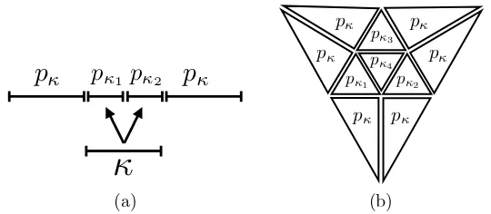
Figure 2. Polynomial degree distribution employed for the
com-petitivehp–refinements: (a) One–dimension; (b) Two–dimensional triangular element.
With the definition of ˜E′κ(·) given in (4.6), we now outline the proposed compet-itive refinement strategy on elementκ, κ∈ T. Firstly, we compute the predicted energy functional reduction whenp–refinement is employed, i.e.,
(4.7) ∆˜E′κ,p:= ˜E′κ(uhp⋆ )−˜E′κ(u⋆κ,p),
whereu⋆
κ,pis the solution of the local finite element problem: Findu⋆κ,p∈ V(TκN,pp)
such thatu⋆κ,p|∂D(κ)=u⋆hp|∂D(κ) and
(4.8) aD(κ)(u⋆κ,p, v) =ℓD(κ)(v) ∀v∈ V0(TκN,pp);
here,pp|κ′ =pκ+ 1 for allκ′∈ TκN.
Secondly, we also consider a sequence of competitivehp–refinements, such that the number of degrees of freedom associated with the finite element space defined over κis identical to the case when pure p–refinement has been employed. Here, for each element κ ∈ T, we again exploit the same local mesh Tκ,Nref employed
for the computation of the local reference solution u⋆κ,ref. Then for the elements
which result from the isotropic refinement ofκ, we employ local polynomial degrees
pκi, i = 1, . . . , nκ; for the remaining elements stemming from the refinement of
the neighbours of κ, we simply set the local polynomial degree equal to pκ, cf. Fig. 2. For example, in one–dimension, following [11, 29], given an elementκwith polynomial degreepκ, an enrichment ofpκ → pκ+ 1 gives rise to pκ+ 2 degrees of freedom associated with κ. On the other hand, we can now consider the case whenκis uniformly subdivided into two sub-elementsκ1andκ2, i.e.,nκ= 2, with associated polynomial degreespκ1 andpκ2, respectively. To ensure that the number
of degrees of freedom in the underlyinghp–refined finite element space defined over
κ1andκ2is identical to the case when purep–enrichment is undertaken, we require that
pκ1+pκ2 =pκ+ 1.
Hence, there are Nκ,hp =pκ,hp–competitive refinements and one p–refinement in
one–dimension.
p κ
0 2 4 6 8 10 12
N κ
, hp
[image:11.595.200.412.117.281.2]0 20 40 60 80 100 120 140 160 180
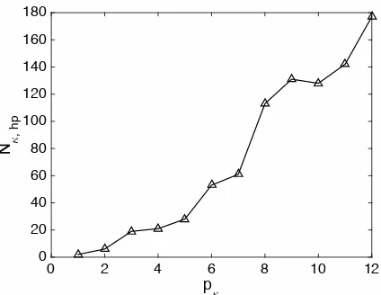
Figure 3. Number of competitive hp–refinements, Nκ,hp, versus
the local polynomial degree pκ when a triangular element κ is isotropically refined.
i= 1, . . . , nκ= 4; as before, the local polynomial degree of the remaining elements stemming from the refinement of the neighbours of κ is set equal to pκ. Let us signify the set of all such polynomial degree distributions onTκ,NrefbyPκ,pκ. Given
that the full space of polynomials has been employed for the p–refinement, the number of degrees of freedom associated withκ is 1/2(pκ+ 2)(pκ+ 3). Then, for
an arbitrary polynomial degree distribution{pκi} 4
i=1 for the sub-elements{κi}4i=1
ofκ, the number of degrees of freedom associated withκis
6 +
3
∑
i=1
[min(pκi, pκ4)−1 + 2(pκi−1)] +
1 2
4
∑
i=1
(pκi−1)(pκi−2),
where we have assumed thatκ4 is the sub-element located at the interior ofκ, cf. Fig. 2(b). Thereby, we select the set ofhp–refinements which satisfy the condition
6 +
3
∑
i=1
[min(pκi, pκ4)−1 + 2(pκi−1)] +
1 2
4
∑
i=1
(pκi−1)(pκi−2) =
1
2(pκ+ 2)(pκ+ 3).
Analogous expressions can also be determined for different element types, other kinds of refinement, e.g., anisotropic refinement, as well as in higher–dimensions. The precise number of competitivehp–refinements, denoted byNκ,hp, is not possible
to determine in a simple closed form expression; instead,Nκ,hpcan be precomputed
for any polynomial order. To this end, in Fig. 3 we present the number of combina-tions of local polynomial degrees{pκi}
4
i=1 with respect topκ in the above setting, i.e., for the case of isotropic refinement of a triangular element in two–dimensions. We notice that the numberNκ,hp of possiblep-configurations is, not surprisingly,
growing as pκ increases. In view of this observation we remark that, although the subsequent local discrete problems defined on each corresponding (patchwise)
maximum Nmax. For example, a random selection of Nmax samples may be con-sidered, cf. Section 5 below; alternatively, a more sophisticated strategy selecting polynomial degree distributions with limited variations could be employed.
We now writeV(Tκ,Nref,phpi),i= 1, . . . , Nκ,hp, to denote the finite element space
based on employing the local (refined) meshTκ,Nrefand some local polynomial degree distributionphpi ∈Pκ,pκ. Thereby, the following competitive hp–refinements may
be defined: Findu⋆
κ,hpi ∈ V(T
N
κ,ref,phpi) such thatu
⋆
κ,hpi|∂D(κ)=u
⋆
hp|∂D(κ) and
(4.9) aD(κ)(uκ,⋆hpi, v) =ℓD(κ)(v) ∀v∈ V0(Tκ,Nref,phpi),
for i = 1, . . . , Nκ,hp. For each local competitive hp–refinement, we compute the
estimated local energy reduction
(4.10) ∆˜E′κ,hp i := ˜E
′
κ(u ⋆
hp)−˜E′κ(u ⋆ κ,hpi),
for i = 1, . . . , Nκ,hp. In this way, for each element κ ∈ T, we may compute the
maximum local predicted error reduction
(4.11) ∆˜E′κ,max= max {
∆˜E′κ,p, max i=1,...,Nκ,hp
∆˜E′κ,hp i
}
,
with ∆˜E′κ,pfrom (4.7). Finally, we refine the set of elements κ∈ T which satisfy the condition
(4.12) ∆˜E′κ,max> θmax κ∈T ∆˜E
′
κ,max,
where 0< θ <1 is a given parameter, cf. [11, 29]. On the basis of [11, 29], through-out this article, we set θ =1/3. The above competitivehp–refinement strategy is
summarised in Algorithm 1.
5. Numerical Examples
In this section we present a series of numerical experiments to demonstrate the practical performance of the proposedhp–adaptive refinement strategy outlined in Algorithm 1.
5.1. Example 1: Linear Elliptic Problem. In this first example, we consider a one–dimensional problem defined over the domain Ω = (0,1). Moreover, we set
µ(ux) =1/2ε u2x, ε > 0, g(u) =1/2u2, and f(x) = 1; this is equivalent to solving the linear elliptic boundary value problem:
−εu⋆xx+u⋆= 1, x∈Ω,
subject to homogeneous Dirichlet boundary conditions. We note that the analytical solution is given by
u⋆(x) = e
−1/√ε−1
e1/√ε−e−1/√εe
x/√ε+ 1−e 1/√ε
e1/√ε−e−1/√εe
−x/√ε+ 1.
In particular, for 0< ε≪1, the analytical solutionu⋆contains boundary layers in the vicinity ofx= 0 andx= 1, cf. [33]; as in [33], we setε= 10−5.
Algorithm 1Competitivehp-adaptive refinement procedure
1: Choose a coarse initial mesh T0 of Ω and a corresponding low-order starting
polynomial degree vectorp0. Setn= 0.
2: Solve (3.1) foru⋆
hp∈ V(Tn,pn).
3: foreach elementκ∈ Tn do
4: Construct the local reference meshTκ,Nref.
5: Compute the local finite element reference solutionu⋆
κ,ref ∈ V(Tκ,Nref,pref)
satisfying (4.5).
6: Compute the local finite elementp–enriched solutionu⋆
κ,p∈ V(TκN,pp) sat-isfying (4.8), together with the corresponding predicted energy functional reduction ∆˜E′κ,p, cf. (4.7).
7: fori= 1, . . . , Nκ,hp do
8: Compute the local competitive hp–refined finite element solutions
u⋆
κ,hpi ∈ V(Tκ,Nref,phpi) satisfying (4.9), together with their respective
predicted energy functional reduction ∆˜E′κ,hp
i defined in (4.10). 9: end for
10: Compute the maximum local predicted error reduction ∆˜E′κ,max, cf. (4.11).
11: end for
12: Determine the set of elements Kn which are flagged for refinement, based on the criterion (4.12).
13: Perform p– or hp–refinement on each κ ∈ Kn according to which refinement takes the maximum in (4.11). This results in a refined global finite element spaceV(Tn+1,pn+1).
14: Setn←n+ 1, and goto Line2.
15: After sufficiently many iterations have been performed output the final solution
u⋆hp∈ V(Tn,pn).
error, with respect to the total number of degrees of freedom employed within the finite element spaceV(T,p), on a linear–log scale; here,
∥v∥2E= ∫ 1
0
(εvx2+v2)dx.
From Fig. 4(a), (b), & (c), we observe, that after an initial transient, the conver-gence lines for each error measure become (on average) straight, thereby indicat-ing exponential convergence of the quantities |E(u⋆)−E(u⋆
hp)|, ∥u
⋆−u⋆
hp∥E, and ∥u⋆−u⋆
hp∥L2(Ω), respectively, asV(T,p) is adaptively enriched. Finally, in Fig. 4(d)
we show thehp–mesh distribution after 9 adaptive refinements. Here, we observe that the algorithm clearly identifies the location of the boundary layers present in the analytical solution u⋆; indeed, in these regions, local subdivision of the mesh has first been employed, followed by subsequentp–enrichment, cf. [33].
5.2. Example 2: Strongly monotone quasilinear PDE. In this second exam-ple, we let Ω be the L-shaped domain (−1,1)2\[0,1)×(−1,0], and set
µ(∇u) =1 2
(
|∇u|2−e−|∇u|2 )
Degrees of Freedom
0 20 40 60 80 100 120
|E(u
*)-E(u
* hp
)|
10-20 10-15 10-10 10-5 100
Degrees of Freedom
0 20 40 60 80 100 120
||u
*-u * hp
||E
10-10 10-8 10-6 10-4 10-2 100
(a) (b)
Degrees of Freedom
0 20 40 60 80 100 120
||u
*-u
* hp
||L 2(Ω
)
10-10 10-8 10-6 10-4 10-2 100
x
0 0.2 0.4 0.6 0.8 1
pκ
0 1 2 3 4 5 6 7
[image:14.595.131.499.99.426.2](c) (d)
Figure 4. Example 1. Comparison of the error with respect to the
number of degrees of freedom: (a)|E(u⋆)−E(u⋆
hp)|; (b)∥u⋆−u⋆hp∥E;
(c) ∥u⋆−u⋆hp∥L2(Ω). (d) hp–Mesh distribution after 9 adaptive
refinements.
Thereby, the corresponding Euler–Lagrange equation for the underlying minimisa-tion problem corresponds to the strongly monotone quasilinear PDE given by:
−∇ ·((1 + e−|∇u⋆|2 )
∇u⋆
)
=f, in Ω.
(5.1)
We selectf and appropriate inhomogeneous Dirichlet boundary conditions so that the analytical solution to (5.1) is given by
u=r2/3sin(2 3φ
)
,
where (r, φ) denote the system of polar coordinates, cf. [10, 20], for example. Selecting the energy norm∥ · ∥E to be the standard H1(Ω) norm, in Fig. 5 we
again present the convergence history of the error in the computed energy func-tional E, together with ∥u⋆−u⋆hp∥E, and ∥u⋆ −u⋆hp∥L2(Ω), as the finite element
(Degrees of Freedom)1/3
0 5 10 15 20
|E(u
*)-E(u *)|hp
10-8 10-6 10-4 10-2 100
hp-refinement 10 MC samples 15 MC samples
(Degrees of Freedom)1/3
0 5 10 15 20
||u
*-u * hp
||E
10-4
10-3
10-2
10-1
100
hp-refinement 10 MC samples 15 MC samples
(a) (b)
(Degrees of Freedom)1/3
0 5 10 15 20
||u
*-u *||hp
L
2(Ω
)
10-6
10-5
10-4
10-3
10-2
10-1
hp-refinement 10 MC samples 15 MC samples
[image:15.595.132.494.112.429.2](c)
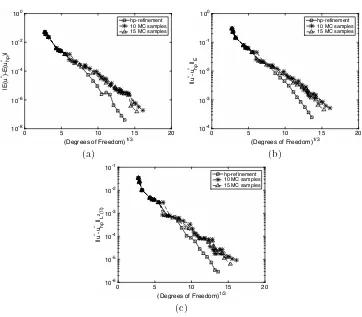
Figure 5. Example 2. Comparison of the error with respect to the
third root of the number of degrees of freedom: (a)|E(u⋆)−E(u⋆
hp)|;
(b)∥u⋆−u⋆
hp∥E; (c) ∥u⋆−u⋆hp∥L2(Ω).
analogous results in the case when a Monte Carlo (MC) approach is employed to limit the number Nmax of hp–refinement samples considered on each element.
More precisely, we randomly select samples based on employing Nmax = 10 and Nmax= 15; in each case two typical realisations are presented. Here, we observe a
slight degradation of the rate of convergence in each of the above error quantities as ourhp–refinement procedure progresses, as we would expect; however, in each case exponential convergence is retained when this simple selection principle is ex-ploited. As noted in Section 4.2 more sophisticated selection principles may also be employed.
-1 -0.5 0 0.5 1 -1
-0.8 -0.6 -0.4 -0.2 0 0.2 0.4 0.6 0.8 1
2 2.5 3 3.5 4 4.5 5 5.5 6
(a)
-0.015 -0.01 -0.005 0 0.005 0.01 0.015
-0.015 -0.01 -0.005 0 0.005 0.01 0.015
2 2.5 3 3.5 4 4.5 5 5.5 6
[image:16.595.197.416.106.486.2](b)
Figure 6. Example 2. (a)hp–Mesh distribution after 18 adaptive
refinements; (b) Zoom of (a).
5.3. Example 3: p–Laplacian. In this final example, forp>1, we consider the
p–Laplacian problem
(5.2) −∇ ·(|∇u⋆|p−2∇u⋆) =f, in Ω = (0,1)2,
subject to inhomogeneous Dirichlet boundary conditions. We point out that in this setting, (5.2) corresponds to the Euler–Lagrange equation for the energy minimi-sation problem
min u∈W01,p(Ω)
{ 1
p
∫
Ω
|∇u|pdx−
∫
Ω f udx
} ;
i.e., we have µ(∇u) = 1/p|∇u|p and g = 0. We select f, and impose suitable
inhomogeneous Dirichlet boundary conditions, so that the analytical solution of (5.2) is given by
(Degrees of Freedom)1/3
4 6 8 10 12
|E(u
*)-E(u
* hp
)|
10-8 10-6 10-4 10-2
hp-refinement 30 MC samples
(Degrees of Freedom)1/3
4 6 8 10 12
||u
*-u
* hp
||W
1,3
(
Ω
)
10-3
10-2
10-1
hp-refinement 30 MC samples
(a) (b)
(Degrees of Freedom)1/3
4 6 8 10 12
||u
*-u * hp
||L
3(Ω
)
10-5 10-4 10-3
10-2 hp-refinement
30 MC samples
[image:17.595.135.497.107.424.2](c)
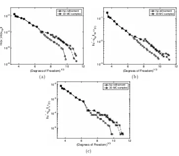
Figure 7. Example 3. Comparison of the error with respect to the third root of the number of degrees of freedom: (a)|E(u⋆)−E(u⋆
hp)|;
(b)|u⋆−u⋆
hp|W1,3(Ω); (c)∥u⋆−u⋆hp∥L3(Ω).
As in [1], throughout this section, we set p = 3 and α= 3/4, which implies that u⋆∈Wβ−ϵ,3(Ω), whereβ=13/6andϵ >0 is arbitrarily small.
In Fig. 7 we plot|E(u⋆)−E(u⋆
hp)|,∥u
⋆−u⋆
hp∥W1,3(Ω), and∥u⋆−u⋆hp∥L3(Ω), with
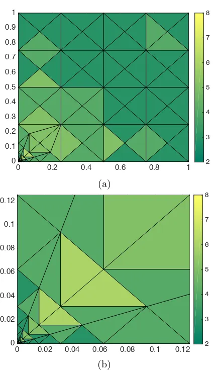
respect to the third root of the number of degrees of freedom in V(T,p). As in the previous examples, we again observe exponential convergence of each of the above error measures, as the finite element space ishp–adaptively modified. Here, we also consider the case when Nmax = 30 random samples are selected; as in the previous example, we again see that exponential convergence of each of the above error quantities is retained, though the rate of convergence is inferior when compared to the case when all potential trial hp–refinements are considered. The final hp–mesh distribution is shown in Fig. 8; as in the previous examples, the adaptive algorithm clearly identifies the location of the singularity present within the analytical solutionu⋆, wherebyh–refinement is undertaken.
6. Conclusions
0 0.2 0.4 0.6 0.8 1 0
0.1 0.2 0.3 0.4 0.5 0.6 0.7 0.8 0.9 1
2 3 4 5 6 7 8
(a)
0 0.02 0.04 0.06 0.08 0.1 0.12
0 0.02 0.04 0.06 0.08 0.1 0.12
2 3 4 5 6 7 8
[image:18.595.202.415.112.481.2](b)
Figure 8. Example 3. (a)hp–Mesh distribution after 23 adaptive refinements; (b) Zoom of (a).
In particular, the underlying adaptive algorithm exploits a competitive refinement technique which seeks to maximise the decrease in the elemental contribution to the total energy based on employing localp– and hp–enrichments of the finite element space. Whilst our approach has been successfully applied to a range of second– order quasilinear problems in both one– and two–dimensions, we emphasise that it is immediately extensible to more general variational-based PDE problems. Future work will be concerned with exploiting anisotropichp–mesh adaptation.
References
1. M. Ainsworth and D. Kay,The approximation theory for the p-version finite element method and application to non-linear elliptic PDEs, Numer. Math.82(1999), 351–388.
3. M. Ainsworth and B. Senior,An adaptive refinement strategy forhp-finite element computa-tions, Appl. Numer. Math.26(1998), no. 1–2, 165–178.
4. I. Babuˇska and B. Q. Guo, Regularity of the solution of elliptic problems with peicewise analytic data. Part I. Boundary value problems for linear elliptic equation of second order, SIAM J. Math. Anal.19(1988), 172–203.
5. I. Babuˇska and M. Suri, The hp–version of the finite element method with quasiuniform meshes, RAIRO Anal. Num´er.21(1987), 199–238.
6. ,The treatment of nonhomogeneous Dirichlet boundary conditions by thep–version of the finite element method, Numer. Math.55(1989), 97–121.
7. ,Thepandh-pversions of the finite element method, basic principles and properties, SIAM Review36(1994), 578–632.
8. R. Becker and R. Rannacher,An optimal control approach to a-posteriori error estimation in finite element methods, Acta Numerica (A. Iserles, ed.), Cambridge University Press, 2001, pp. 1–102.
9. C. Bernardi, N. Fi´etier, and R. G. Owens,An error indicator for mortar element solutions to the Stokes problem, IMA J. Numer. Anal.21(2001), no. 4, 857–886.
10. S. Congreve, P. Houston, and T. P. Wihler,Two-gridhp–version discontinuous Galerkin finite element methods for second-order quasilinear elliptic PDEs, J. Sci. Comput.55(2013), no. 2, 471–497.
11. L. Demkowicz,Computing withhp-adaptive finite elements. Vol. 1, Chapman & Hall/CRC Applied Mathematics and Nonlinear Science Series, Chapman & Hall/CRC, Boca Raton, FL, 2007, One and two dimensional elliptic and Maxwell problems.
12. L. Demkowicz, W. Rachowicz, and Ph. Devloo,A fully automatichp–adaptivity, J. Sci. Com-put.17(2002), no. 1-4, 117–142.
13. W. D¨orfler and V. Heuveline,Convergence of an adaptivehpfinite element strategy in one space dimension, Appl. Numer. Math.57(2007), no. 10, 1108–1124.
14. T. Eibner and J. M. Melenk,An adaptive strategy forhp-FEM based on testing for analyticity, Comput. Mech.39(2007), no. 5, 575–595.
15. K. Eriksson, D. Estep, P. Hansbo, and C. Johnson, Introduction to adaptive methods for differential equations, Acta Numerica (A. Iserles, ed.), Cambridge University Press, 1995, pp. 105–158.
16. E. H. Georgoulis, E. Hall, and P. Houston,Discontinuous Galerkin methods onhp–anisotropic meshes II: A posteriori error analysis and adaptivity, Appl. Numer. Math.59(9) (2009), 2179–2194.
17. S. Giani and P. Houston,Anisotropichp–adaptive discontinuous Galerkin finite element meth-ods for compressible fluid flows, Int. J. Numer. Anal. Model.9(2012), no. 4, 928–949. 18. P. Houston and E. S¨uli,Adaptive finite element approximation of hyperbolic problems,
Er-ror Estimation and Adaptive Discretization Methods in Computational Fluid Dynamics. Lect. Notes Comput. Sci. Engrg. (T. Barth and H. Deconinck, eds.), vol. 25, Springer, 2002, pp. 269–344.
19. P. Houston and E. S¨uli, A note on the design of hp–adaptive finite element methods for elliptic partial differential equations, Comput. Methods Appl. Mech. Engrg.194(2-5)(2005), 229–243.
20. P. Houston, E. S¨uli, and T. P. Wihler,A posteriori error analysis ofhp-version discontinuous Galerkin finite element methods for second-order quasi-linear PDEs, IMA J. Numer. Anal.
28(2007), no. 2, 245–273.
21. G. E. Karniadakis and S. Sherwin,Spectral/hpfinite element methods in cfd, Oxford Univer-sity Press, 1999.
22. C. Mavriplis, Adaptive mesh strategies for the spectral element method, Comput. Methods Appl. Mech. Engrg.116(1994), no. 1-4, 77–86, ICOSAHOM’92 (Montpellier, 1992). 23. J. M. Melenk and B. I. Wohlmuth,On residual-based a posteriori error estimation inhp-FEM,
Adv. Comp. Math.15(2001), 311–331.
24. W. F. Mitchell and M. A. McClain,A comparison ofhp-adaptive strategies for elliptic partial differential equations, ACM Transactions on Mathematical Software (TOMS)41(2014), 2:1– 2:39.
26. P. H. Rabinowitz,Minimax methods in critical point theory with applications to differential equations, CBMS Regional Conference Series in Mathematics, vol. 65, Published for the Con-ference Board of the Mathematical Sciences, Washington, DC; by the American Mathematical Society, Providence, RI, 1986.
27. W. Rachowicz, J. T. Oden, and L. Demkowicz,Toward a universalhp-adaptive finite element strategy. Part 3: Design of hpmeshes, Comput. Methods Appl. Mech. Engrg. 77(1989), 181–212.
28. C. Schwab,p- and hp-FEM – Theory and application to solid and fluid mechanics, Oxford University Press, Oxford, 1998.
29. P. Solin, K. Segeth, and I. Dolezel,Higher-order finite element methods, Studies in advanced mathematics, Chapman &Hall/CRC, Boca Raton, London, 2004.
30. B. Szab´o and I. Babuˇska,Finite element analysis, J. Wiley & Sons, New York, 1991. 31. J. Valenciano and R. G. Owens,An h-p adaptive spectral element method for Stokes flow,
Appl. Numer. Math.33(2000), no. 1-4, 365–371.
32. R. Verf¨urth,A review of a posteriori error estimation and adaptive mesh-refinement tech-niques, B.G. Teubner, Stuttgart, 1996.
33. T. P. Wihler,Anhp-adaptive strategy based on continuous Sobolev embeddings, J. Comput. Appl. Math.235(2011), 2731–2739.
34. E. Zeidler,Nonlinear functional analysis and its applications. III, Springer-Verlag, New York, 1985, Variational methods and optimization, Translated from the German by L. F. Boron. MR 768749 (90b:49005)
35. ,Nonlinear functional analysis and its applications. II/B, Springer-Verlag, New York, 1990, Nonlinear monotone operators, Translated from the German by the author and L. F. Boron. MR 1033498 (91b:47002)
School of Mathematical Sciences, University of Nottingham, University Park, Not-tingham, NG7 2RD, UK
E-mail address:Paul.Houston@nottingham.ac.uk
Mathematisches Institut, Universit¨at Bern, Sidlerstrasse 5, CH-3012 Bern, Switzer-land