Wide angle search for extrasolar planets by the transit method

(1)

WIDE ANGLE SEARCH FOR EXTRASOLAR PLANETS BY THE

TRANSIT METHOD

Khalid Alsubai

A Thesis Submitted for the Degree of PhD

at the

University of St. Andrews

2008

Full metadata for this item is available in the St Andrews

Digital Research Repository

at:

https://research-repository.st-andrews.ac.uk/

Please use this identifier to cite or link to this item:

http://hdl.handle.net/10023/521

This item is protected by original copyright

This item is licensed under a

(2)

Wide Angle Search for Extrasolar planets

by the Transit Method

Khalid Alsubai, Bsc, Msc

School of Physics and Astronomy

University of St Andrews

Submitted for the degree of Ph.D.

(3)

2

DECLARATION

I, Khalid Alsubai, hereby certify that this thesis, which is approximately 50000 words in length, has been written by me, that it is the record of work carried out by me and that it has not been submitted in any previous application for a higher degree. The English in this thesis has been corrected by professional proof readers for grammatical errors only.

Date ... Signature Of Candidate ...

I was admitted as a research student in January 2002 and as a candidate for the degree of Ph.D. in January 2002; the higher study for which this is a record was carried out in the University of St. Andrews between January 2002 and January 2008.

Date ... Signature Of Candidate ...

I hereby certify that the candidate has fulfilled the conditions of the Resolution and Regulations appropriate for the degree of Ph.D. in the University of St. Andrews and that the candidate is qualified to submit this thesis in application for that degree.

Date ... Signature Of Supervisor ...

In submitting this thesis to the University of St. Andrews I understand that I am giving per-mission for it to be made available for use in accordance with the regulations of the University Library for the time being in force, subject to any copyright vested in the work not being affected thereby. I also understand that the title and abstract will be published, and that a copy of the work may be made and supplied to any bona fide library or research worker.

(4)

ABSTRACT

The transit method is considered to be one of the most promising for discovering extrasolar plan-ets. However, the method requires photometric precision of better than_∼1%. If we are able to achieve this kind of accuracy, then we are set to discover extrasolar planets. The uniqueness of my experiment will lead to the discovery of transiting planets around the brightest and most important stars quicker than the competitors in the field. The importance of the transit method stems from being able to supply many more planetary parameters than other methods which plays a crucial role in testing planet formation theories. This thesis is divided into eight chapters.

(5)

(6)

1 Extrasolar Planets 15

1.1 The Transit Method . . . 15

1.2 Known Transiting Planets . . . 19

1.2.1 HD 209458 b . . . 19

1.2.2 Successful Ground-based Transit Search Experiments . . . 19

1.2.3 Space-based Transit Search Experiments: . . . 21

1.2.4 Using Transits to Determine Accurate Planet Radii . . . 22

1.2.5 Using Transits to Detect and Characterise an Extrasolar Planet Atmosphere 22 1.3 The Radial Velocity Method . . . 25

1.4 The Microlensing Method . . . 26

1.5 Detection via Direct Imaging . . . 27

1.6 The Pulsar Timing Method . . . 28

1.7 The Formation of Hot Jupiters . . . 29

1.8 Observed Properties of Extrasolar Planets . . . 30

1.8.1 Planet Eccentricities . . . 30

1.8.2 The Mass Function . . . 32

1.8.3 Metal Rich Stars . . . 33

2 Design of the PASS0 Experiment 37 2.1 Introduction . . . 37

2.2 CCD Signal and Noise Modelling . . . 37

2.2.1 Readout Noise . . . 37

2.2.2 Bias Level . . . 37

2.2.3 Bias Pattern . . . 38

2.2.4 Dark Current . . . 38

2.2.5 Photons . . . 38

2.2.6 Pixel Noise . . . 39

2.2.7 Measuring the CCD Gain . . . 40

2.2.8 Signal-to-Noise Ratio . . . 40

2.2.9 Lightcurve Noise . . . 42

2.3 PASS: Permanent All Sky Survey . . . 44

2.3.1 The Motivation and Ideas Behind PASS . . . 44

2.3.2 PASS0: A Prototype PASS Experiment . . . 45

(7)

6 CONTENTS

2.3.3 Essential Considerations for Successful Non-Tracking Observations . . . 51

2.3.4 Trailing and its Effect on Signal-To-Noise . . . 55

2.3.5 Optimal Exposure Time for PASS0 . . . 57

2.3.6 Limitations due to Scintillation . . . 58

2.3.7 A Theoretical Pass0 Noise Model . . . 59

2.3.8 The Advantages of PASS0 . . . 60

2.3.9 The Disadvantages of PASS0 . . . 61

2.3.10 The First Pass0 Observation Run . . . 61

3 PASS0 Data Reduction 63 3.1 The PASS0 Image Processing Pipeline . . . 63

3.1.1 Stage 0: Preprocessing Calibrations . . . 63

3.1.2 Stage 1: Reference Images and Astrometry . . . 66

3.1.3 Stage 2: Image Subtraction . . . 69

3.1.4 Stage 3: Measuring Difference Fluxes . . . 71

3.1.5 Stage 4: Constructing the lightcurves: . . . 72

3.2 Lightcurve Calibration . . . 74

3.2.1 The String Method . . . 77

3.2.2 PASSCAL . . . 79

3.3 HD209458 . . . 83

4 Optimising SuperWASP Photometry 87 4.1 The SuperWASP Experiment . . . 87

4.2 SuperWASP Observations and Reductions . . . 87

4.3 Application of the PASS0 Pipeline . . . 89

4.3.1 Adapting the PASS0 Pipeline . . . 89

4.3.2 Comparing the Gaussian Preconvolution Tests . . . 94

4.3.3 Testing the PASS0 Pipeline on Fake Image Data . . . 98

4.3.4 Sub-Pixel Phase Map . . . 101

4.3.5 Choosing the Best Gaussian Preconvolution . . . 101

4.3.6 Image Subtraction Residuals . . . 102

4.3.7 Further Lightcurve Calibration . . . 103

4.4 Comparing the PASS0 and SuperWASP Pipeline Results . . . 107

4.4.1 Comparing RMS Diagrams . . . 107

4.4.2 Comparing the Lightcurves of XO-1 . . . 109

5 Variable Candidates 113 5.1 Introduction . . . 113

5.2 Variables in the PASS0 Lightcurve Data . . . 113

5.2.1 Identifying Variable Stars . . . 113

5.2.2 Determining the Period of the Variable Stars . . . 116

5.3 Variables in the SuperWASP Lightcurve Data . . . 118

(8)

6 Transit Candidates 131

6.1 Introduction . . . 131

6.2 Transit Search Algorithms . . . 131

6.3 Transit Candidates in the PASS0 Lightcurve Data . . . 132

6.4 Transit Candidates in the SuperWASP Lightcurve Data . . . 141

6.5 Conclusions . . . 143

7 WASP-7b and WASP-8b 147 7.1 Introduction . . . 147

7.2 Reductions . . . 147

7.3 Comparing the Lightcurves from the PASS0 and SuperWASP Pipelines . . . 152

7.4 Fitting the Lightcurves from the PASS0 and SuperWASP Pipelines . . . 161

7.5 Conclusions . . . 162

8 Summary 163

A Relation between Gaussian Sigma and FWHM 167

B Number of Effective Pixels of a Gaussian PSF 169

(9)

(10)

2.1 PASS0 CCD And Lens Evaluation . . . 48

2.2 PASS0 And SWASP Star Counts . . . 49

4.1 Gaussian convolution kernels . . . 94

4.2 Final RMS Diagram Fits . . . 107

5.1 PASS0 Variable Star Properties . . . 124

5.2 PASS0 Variable Star Properties . . . 125

5.3 SuperWASP Variable Star Properties . . . 130

7.1 Pipeline Comparison for WASP-7b . . . 151

7.2 Pipeline Comparison for WASP-8b . . . 151

7.3 Fitted Planet Parameters for WASP-7b and WASP-8b . . . 160

(11)

(12)

1.1 Geometry Of A Transit . . . 16

1.2 Transit Of HD209458 . . . 17

1.3 Transit Duration . . . 18

1.4 Transits Of HD209458 In Different Bandpasses . . . 23

1.5 Phased Infrared Planet Flux . . . 24

1.6 Radial Velocity Curve Of HD209458 . . . 25

1.7 Microlens Diagram . . . 27

1.8 OGLE-05-390Lb . . . 28

1.9 Eccentricity Against Orbital Size . . . 30

1.10 Planet Mass Against Eccentricity . . . 31

1.11 Eccentricity Against Period . . . 32

1.12 Planet Mass and Period Histogram . . . 33

1.13 Planet Mass Against Orbital Size . . . 34

1.14 Planet Distribution As A Function Of Metallicity . . . 36

2.1 Theoretical Signal-To-Noise Versus Exposure Time . . . 41

2.2 PASS Design Concept . . . 44

2.3 The PASS0 Camera In Tenerife . . . 50

2.4 PASS0 Vignetting . . . 52

2.5 PASS0 Sample Images And PSF . . . 53

2.6 Example Trailing Apertures . . . 54

2.7 S/N For A Single Trailed Observations . . . 56

2.8 Total S/N For Many Trailed Observations . . . 57

2.9 PASS0 Optimal Exposure Time . . . 58

2.10 Scintillation Noise . . . 59

2.11 PASS0 Theoretical RMS Diagram . . . 60

3.1 The PASS0 PSF . . . 64

3.2 FWHM and Sky Trends for PASS0 Data . . . 65

3.3 DAOPhot Roundness Versus PASS0yPixel Coordinate . . . 67

3.4 Star Trails On PASS0 . . . 68

3.5 Illustration Of Triangle Matching . . . 70

3.6 PASS0 Difference Imaging Residuals . . . 73

(13)

12 LIST OF FIGURES

3.7 PASS0 Pipeline Flow Chart . . . 75

3.8 PASS0 Lightcurve Calibrations With The String Method . . . 76

3.9 RMS Diagrams For PASS0 Data . . . 78

3.10 PASSCAL Patterns For PASS0 Lightcurves . . . 81

3.11 PASS0 Lightcurve Calibrations WithPASSCAL . . . 82

3.12 Phased Lightcurves Of HD209458 . . . 85

4.1 Blending Characterisation In SuperWASP . . . 88

4.2 The SuperWASP PSF . . . 90

4.3 SuperWASP Difference Image Subregion . . . 91

4.4 SuperWASP Difference Image . . . 92

4.5 RMS Diagram For Different Blur Tests . . . 95

4.6 Noise Parameters Versus Gaussian FWHM . . . 96

4.7 RMS Scatter Versus Gaussian FWHM . . . 97

4.8 Recovered Reference Fluxes From Fake Image Data . . . 99

4.9 Recovered Difference Fluxes From Fake Image Data . . . 100

4.10 SuperWASP Sub-Pixel Phase Maps . . . 102

4.11 SuperWASP Difference Image Residuals . . . 104

4.12 Tamuz Coefficients . . . 105

4.13 RMS Diagrams For SuperWASP Data . . . 108

4.14 Comparing Final Accuracy Results . . . 109

4.15 Lightcurves Of XO-1 . . . 111

4.16 Phased Lightcurves Of XO-1 . . . 112

5.1 Histogram of the Number of Epochs in the PASS0 Lightcurves . . . 114

5.2 RMS Diagram to Identify Variable Stars in the PASS0 Data . . . 115

5.3 Normalised Cumulative Histogram of Lightcurve RMS . . . 116

5.4 Example PASS0 Lightcurve Periodograms . . . 117

5.5 Unphased PASS0 Variable Star Lightcurves . . . 120

5.6 Unphased PASS0 Variable Star Lightcurves . . . 121

5.7 Phased PASS0 Variable Star Lightcurves . . . 122

5.8 Phased PASS0 Variable Star Lightcurves . . . 123

5.9 RMS Diagram to Identify Variable Stars in the SuperWASP Data . . . 126

5.10 Normalised Cumulative Histogram of Lightcurve RMS . . . 127

5.11 Unphased SuperWASP Variable Star Lightcurves . . . 128

5.12 Phased SuperWASP Variable Star Lightcurves . . . 129

6.1 AoVtr Statistic Versus Magnitude ForNH= 15 . . . 133

6.3 Transit Candidates forNH= 15 . . . 137

(14)

7.1 RMS Diagrams for WASP-7b . . . 149

7.2 RMS Diagrams for WASP-8b . . . 150

7.3 Unfiltered Lightcurve for WASP-7b . . . 154

7.4 Unfiltered Lightcurve for WASP-8b . . . 155

7.5 Lightcurve Correlations for WASP-7b . . . 156

7.6 Lightcurve Correlations for WASP-8b . . . 157

7.7 Lightcurve for WASP-7b . . . 158

(15)

(16)

Transit Detection And Observed

Properties Of Extrasolar Planets

The prime experiment that we report in this thesis is based on the aim of detecting extrasolar planets using the transit method. However, there are many available methods to detect extrasolar planets and a number of them have already had success in planet detections, some being more successful to date than others. In the introduction to the thesis we discuss in relative detail only the transit method (central to the thesis), the radial velocity method (the most successful method to date) and the microlensing method (which is starting to yield planets). Some other methods are not mentioned but the list is not complete since the aim of this thesis is not to review the whole field of extrasolar planets.

1.1 The Transit Method

When a planet passes in front of its parent star it blocks part of the star flux. To observe such a phe-nomenon from another star system at a great distance from the planet, the observer has to be within a very restricted region of space. Therefore any planet around a star does not necessarily transit its host and we will only observe a small fraction of planets as transiting planets. The decrease in luminosity of the host star when the planet transits is also of the order of∼1% for a Jupiter-sized planet around a solar-type star which requires high photometric precision observations carried out during and after the transit event.

In the following analysis of the transit phenomena we will assume that planetary orbits are circular and that the surface brightness, mass, and radius of the planet are small compared to that of the parent star. We will also assume that the orbital radius is much larger than the size of the parent star itself.

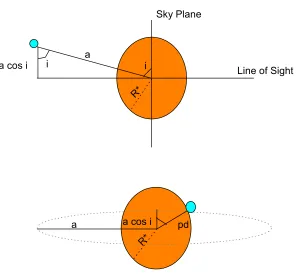
A planet with radiusRPorbits a star of radiusR∗and massM∗at an orbital radiusa. A transit

of the stellar disk will be seen by an observer only if the orbital plane is at the correct inclination to the line of sight (see Figure 1.1). Mathematically the inclinationimust satisfy the following:

acosi_≤R∗+RP (1.1)

(17)

16 CHAPTER 1. EXTRASOLAR PLANETS R * R * R * Sky Plane

Line of Sight a

i

i a cos i

a

R *

a cos i

R *

[image:17.595.137.436.115.393.2]

pd

Figure 1.1: The geometry of a transit event of inclinationiand orbital radiusaas seen from the side (top) and from the observer’s point of view (bottom) at a moment when the planet lies at a projected distanced(t)from the star centre.

Sincecosiis the projection of the vector perpendicular to the orbital plane onto the hemisphere of the sky and this is distributed uniformly over the surface of the sky hemisphere, it is equally likely to take on any random value between 0 and 1. Therefore, for a set of planetary systems with arbitrary orientation with respect to the observer [69], the probability that the inclination satisfies the necessary geometry for a transit is given by:

Geometric Transit Probability=

R(R∗₊_RP)/a

0 d(cosi)

R1

0 d(cosi)

= R∗+RP

a ≈

R∗

a (1.2)

The photometric depth of a transiting planet is determined by the fraction of the light from the star that is eclipsed. Assuming that the flux from the star isF before or after the transit, and that the planet creates a change in flux of∆F, then the ratio of∆F toF can be calculated by considering the ratio of the area of the planetary disk to that of the stellar disk as follows:

(18)

[image:18.595.86.476.113.434.2]

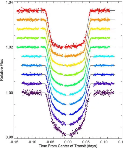
Figure 1.2: The transit lightcurve of HD209458b, taken from Charbonneau et al. 2000 [14].

This equation ignores the effect of limb darkening, and shows that the luminosity of the host star during transit is reduced by the square of the ratio of planet to star radius.

Figure 1.2 shows an typical transit lightcurve. In fact it is the discovery lightcurve for the first known transiting planet taken from Charbonneau et al. 2000 [14]. The periodP of the transiting planet can be determined very simply by observing two or more consecutive transits and the period is then simply the time between the transits. The transit itself yields the duration of the event or it can be derived using the theory presented in Figure 1.3. This figure shows that the planet subtends an angle of2θradians during a transit, out of the angle of2πradians that it subtends during a full orbit. The duration of a transittTis therefore given by:

tT=

P θ

π (1.4)

(19)

18 CHAPTER 1. EXTRASOLAR PLANETS

Figure 1.3: The transit duration is set by the fraction of the total orbit (left) for which a portion of the planet eclipses the stellar disk (right).

the impact parameter) isacosiand we may solve for the distancexusing the Pythagorean rule:

x2= (R∗+RP)2−(acosi)2 (1.5)

Then from Figure 1.3(a) we can calculateθusing simple trigonometry as:

θ= arcsin

p

(R∗+RP)2−(acosi)2

a

!

(1.6)

Rewriting the equation for transit duration (Equation 1.4) using Equation 1.6 and assuming thatθis a small angle such thatsinθ_≈θ, then we get:

tT =

Pp

(R∗+RP)2−(acosi)2

πa (1.7)

For the situation thata≫R∗ ≫RP, which is generally true, Equation 1.7 becomes:

tT =

P π

s

R∗ a

2

−cos2_i_≤ P R∗

πa (1.8)

We can get the mass of the host starM∗from spectroscopy to determine the spectral type and

then use the mass-radius relation for (Sun-like) main sequence stars to get the star radiusR∗. It is

known that this relationship is given by the approximation:

R∗=f(M∗)≈M∗ R⊙ M⊙

(1.9)

With the star mass and radius we can then calculate the orbital radius of the planet using Kepler’s law:

P2= 4π

2_a3

GM∗

(20)

The above equations are what are needed to analyse the lightcurve of a transiting planet and can be used to obtain interesting properties like the planet radius and orbital period. The inclination of the orbit of a transiting planet can be obtained from the lightcurve which is very important when combined with the detection of radial velocity variations since it leads to a real estimate of the planet mass, not just a minimum mass estimate (see Section 1.3).

1.2 Known Transiting Planets: HD 209458 b and Others

1.2.1 HD 209458 b

On November 12th 1999, a team led by G. W. Henry, G. Marcy, R. P. Butler and S. S. Vogt, announced the discovery of the first transiting planet around the star HD209458 (IAU Circular 7307). In fact the discovered planet had been observed previously by Brown, T and Charbonneau, D. between the 9th to 16th of September 1999 through the STARE project. HD209458 is at 47 parsecs from the Sun in the constellation of Pegasus, and it is very similar to our Sun since it has almost the same mass at∼1.05M⊙and spectral type G0V. The apparent magnitude of the star is

7.65.

The planet was first detected by measuring the radial velocity variations of the star using the Keck telescope. The sinusoidal periodicity in the velocity versus time curve with amplitude

∼81 m/s indicated the presence of a planet. Fits to the curve implied that the mass of the planet is

∼0.62MJUP at an orbital distance of∼0.046 AU (IAU Circular 7307). Photometric observations were carried out at the times of transit predicted from the radial velocity data. These observations reveal a magnitude dip of_∼0.02 mag (or approximately 2%). Both Henry et al. 2000 [32] and Charbonneau et al. 2000 [14] can claim this first detection of a transiting planet, although the Charbonneau et al. data set is much more convincing and reliable since they observed two full transits whereas Henry et al. only observed the start of one transit.

These data allowed the teams to derive a planetary radius of 1.42RJUP, and orbital inclination

sini >0.993. The actual mass of the planet was therefore calculated to be_∼0.62MJUP.

Knowing the mass and radius of the planet we can calculate the density and we get∼0.27 g/m3; this classifies it as a gas giant. The interesting fact is that despite having a mass of only∼62% that of Jupiter, the radius is_∼60% larger than that of Jupiter. This agrees perfectly with theories that anticipated a bloated planet at this close distance to the host star [28].

1.2.2 Successful Ground-based Transit Search Experiments

An up to date list of extrasolar planets is kept at “The Extrasolar Planets Encyclopedia” maintained by J.P. Schneider [102]. The web address for this very valuable resource is http://exoplanet.eu/.

OGLE

The Optical Gravitational Lensing Experiment (OGLE; [88]) uses the 1.3 m Warsaw telescope located at Las Campanas Observatory in Chile. The telescope has an imaging camera with a 4K×4K CCD, and their configuration of the telescope and CCD gives a35′

×35′

(21)

standard microlensing events, but also the data is useful for searching for variables and transiting planets because each field is visited a few and/or many times during one night over many years of observing seasons. In the first few years of the survey, many transit candidates were announced [89] but after a while it became clear that a large fraction of these are systems that have lightcurves mimicking a transiting planet (e.g. [86]). However, as of November 2007, OGLE has lead to the discovery of 7 transiting extrasolar planets close to the Galactic plane (see the website at http://www.astrouw.edu.pl/∼ogle/).

HAT

The Hungarian Automated Telescope Network (HATNet; [5]) uses a 2K_×2K CCD with a 11 cm diameter commercial lens. The FOV is 8×8 square degrees. There are 3 instruments located around the Earth, one at the Fred Lawrence Whipple Observatory (FLWO) in the US, one at the Mauna Kea observatory in Hawaii, and one at the WISE observatory in Israel. As of November 2007, the HAT network has discovered 6 extrasolar planets transiting their parent stars (see the website at http://www.cfa.harvard.edu/∼gbakos/HAT).

SuperWASP

The acronym WASP stands for Wide Angle Search for Planets consortium [79] and it has a very similar concept as that of HAT. The cameras use a similar lens (also commercial) but with a better quality CCD. Currently there are two SuperWASP sites and at each site there are 8 cameras mounted on a single robotic equatorial mount. Each camera has a field of view of 7.8×7.8 square degrees. More details about the SuperWASP experiment and the prototype experiment WASP0 are described at the beginning of Chapter 4. As of November 2007, SuperWASP has discovered 5 extrasolar planets (see the website at http://www.superwasp.org/).

TRES

TRES stands for the Trans-Atlantic Exoplanet Survey [4] and the experiment consists of a network of three small-aperture telescopes searching the sky for transiting planets (Sleuth at the Palomar Observatory, Southern California, USA; PSST at the Lowell Observatory, Northern Arizona, USA; STARE at the Teide Observatory, Canary Islands in Spain). The small telescopes have an f/2.8 lens with a 10 cm aperture that has a field of view of 6×6 degrees coupled with a 2048x2048 back-illuminated CCD. As of November 2007, TRES has discovered 3 planets (see the website at http://www.astro.caltech.edu/∼ftod/tres/tres.html).

XO

(22)

rate removing the need for tracking of observations. As of November 2007, XO has discovered 3 planets (see the website at http://www-int.stsci.edu/∼pmcc/xo/).

1.2.3 Space-based Transit Search Experiments:

SWEEPS

The acronym SWEEPS stands for the Sagittarius Window Eclipsing Extrasolar Planet Search. This team uses the Hubble Space Telescope (HST) to search for transiting planets towards the centre of the Milky Way. This experiment has proved that extrasolar planets can exist anywhere in the Galaxy [70]. However spectroscopic confirmation of the transit candidates via radial velocity mea-surements is a difficult challenge because the faintness of the stars puts them beyond even some of the largest ground-based telescopes. As of November 2007, SWEEPS has discovered 2 transiting planets (see the website at http://www.nasa.gov/mission pages/hubble/exoplanet transit.html).

The COROT Mission

The COROT space mission has two objectives:

• Stellar seismology, or the detection and measurement of stellar vibrations.

• The search for planets around stars other than the Sun.

Both objectives require the same technique of very high precision stellar photometry (one hundred times better than that which can be achieved from the best observatories on Earth), and continuous observations of the same part of the sky over very long periods (at least 150 days). This is impos-sible from the Earth, since the Earth’s orbital motion around the Sun only allows us to observe the same part of the sky for 6 to 8 months. . . and only at night (except at the poles)!

By creating an observing program that consists of observing, in a systematic way, many fields of 12000 stars, it has been estimated that about one hundred hot Jupiter planetary systems can be detected, along with a few dozen small/terrestial planets. The first extrasolar planet detection from COROT was in May of 2007. The planet was named COROT-Exo-1b [101] with an orbital period of∼1.5 d indicating that it is a very hot Jupiter (since it also has a radius of 1.78 times that of Jupiter). The host star is a main sequence star very similar to our Sun. COROT-Exo-1b is the only planet discovered by the COROT mission as of November 2007 (see the website at http://smsc.cnes.fr/COROT/).

The Kepler Mission

The Kepler Mission is specifically designed to survey the extended solar neighborhood to de-tect and characterize hundreds of terrestrial and larger planets in or near the habitable zone, and provide fundamental progress in our understanding of planetary systems. The results will yield a broad understanding of planetary formation, the frequency of formation, the structure of individual planetary systems and the generic characteristics of stars with terrestrial planets.

(23)

to:-22 CHAPTER 1. EXTRASOLAR PLANETS

• Determine the frequency of terrestrial and larger planets in or near the habitable zone; dis-tributions of planet sizes, semi-major axis, albedo, size, mass, and density of short-period giant planets.

• Determine the properties of those stars that harbor planetary systems.

Kepler is predicted to be able to measure stellar flux with a fractional precision of the order of 10−5 _{over the typical transit duration for terrestrial planets (}_∼_{13 hours). The mission will use}

a differential photometer to continuously monitor the brightness of _∼105 dwarf stars for up to 4 years, and hence it is expected to generally see∼4 transits of a terrestrial planet in the habit-able zone of a Sun-like star (since observations are not interrupted by the day-night and seasonal cycle). The launch of the mission is scheduled for the beginning of 2009 (see the website at http://kepler.nasa.gov/).

1.2.4 Using Transits to Determine Accurate Planet Radii

Recently Knuston et al. 2007 [41] gathered 1066 spectra over four distinct transits of HD209458 with the STIS spectrometer on the Hubble Space Telescope with synthesised multiple-bandpass photometry (see Figure 1.4). Assuming the stellar mass-radius relation from Cody & Sasselov 2002 [18], and theoretical models for limb darkening to significantly improve the estimates of the radius and orbital inclination of HD 209458b, they find that the radius of HD 209458b is 1.320_±0.025RJUPwhich is a factor of two more precise than previous measurements. Knutson et al. 2007 find a density for the planet of 0.345±0.05 g/cm3. The planet’s inclination is found to be 86.929◦

±0.010◦

, a factor of three more precise than previous measurements.

The above example is a good illustration of how the transit method can be used to measure accurate planetary radii. From these measurements the planet mass-radius relationship can be accurately explored which is necessary in order to carefully investigate various planet formation scenarios.

1.2.5 Using Transits to Detect and Characterise an Extrasolar Planet Atmosphere

One of the aims of studying extrasolar planets is to learn about the composition of the planet and its atmosphere. By studying the absorption-line spectra of the star during and out of transit, it is possible to construct the absorption line spectra of the planet [12]. This method has been used to detect elements such as C, O and Na in the atmosphere of HD209458 [15] and to learn that HD209458 is losing elements from its atmosphere as it is blown away due to the planet’s proximity to its host star [93]. There is even some evidence that the atmosphere of the planet takes the shape of a comet. For instance, Vidal-Madjar et al. 2003 [92] found that the depth of the transit is_∼15% if the transit is observed at the wavelength of the Lymanα transition of the hydrogen atom (compared to the ∼1.5% dip in visible light). This means that the hydrogen of the planet extends out past the Roche limit and the planet must therefore be losing its atmosphere.

(24)

[image:24.595.80.496.104.605.2]

(25)

[image:25.595.104.474.103.449.2]

Figure 1.5: The normalised infrared flux ofυAndromeda b as a function of orbital phase [30].

the infrared than in the visible, which is what has lead to its successful detection. The planet’s infrared flux confirms its hot temperature at∼1150 K.

The starυAndromeda is orbited by three known planets, the innermost of which has an orbital period of 4.617 days. Again infrared observations with the Spitzer Space Telescope have detected the emission from the hot atmosphere and it was found that the emission varies with the phase of the planet [30]. This indicates that there is a large temperature difference between the day and night side of the planet. Figure 1.5 shows the normalised variation in infrared flux of the planet as a function of phase.

(26)

[image:26.595.117.452.110.378.2]

Figure 1.6: The radial velocity curve of HD209458 taken from Mazeh et al. 2000 [49]

1.3 The Radial Velocity Method

The majority of the known extrasolar planets around main sequence stars have been discovered by the radial velocity method. The method is based on the fact that an orbiting planet perturbs the host star in such a way that the star also orbits the combined centre of mass of the system. The motion of the star creates a Doppler shift in the spectral lines of the star which shifts the lines towards the red when the star is moving away from the observer and shifts the lines towards the blue when the star is moving towards the observer. Since the planetary motion is periodic then so is this Doppler shift.

By observing spectra of the host star over the course of an orbital period, we can measure the radial velocty of the star at various orbital phases from the Doppler shift of the spectral lines relative to some reference lines at rest on the Earth. The radial velocity curve will then look similar to that shown in Figure 1.6 which is taken from a follow-up paper on the discovery of HD209458b by Mazeh et al. 2000 [49]. From the radial velocity curve we can calculate the radial velocity semi-amplitudeKof the star which is related to the star massM∗, planet massMP, inclinationi,

periodP and eccentricityeby the equation:

K=

2πG

P 1/3

MPsini

(MP+M∗)2/3

1

(27)

We may also determineP from the radial velocity curve, and the star massM∗ can be estimated

from determining the spectral type of the host star from the radial velocity spectra.

Also, if we assume a circular orbit (e= 0) and thatMP≪M∗then Equation 1.11 reduces to:

K= 28.4

P

1year

−1/3

MPsini

MJUP

M∗ M⊙

−2/3

m s−1 (1.12)

MeasuringKallows us to calculate the minimum planet massMPsiniand Kepler’s third law in Equation 1.10 can be use to determine the orbital radiusaof the planet. We refer toMPsinias the minimum planet mass sincesinican only take values between 0 and 1 for inclinations between 0◦

and 90◦

which implies thatMPsiniis always smaller thanMP. Note that in the case of a planet with an eccentric orbit, the eccentricity can be determined from the shape of the radial velocity curve by fitting the correct model to the data.

We consider the example of Jupiter orbiting the Sun. This causes a K = 12.5 ms−1

semi-amplitude radial velocity with a period of 11.9 years. In the case of Earth orbiting the Sun,K is about 0.1 ms−1_{. Our current limit on radial velocity accuracy is about}_K _{= 3}_ms−1 _{so Jupiter is}

certainly detectable if we observe for long enough, but Earth is not detectable by this method. Limitations of the radial velocity method include the fact that if the orbital systems that we observe are seen face on (i= 0) then there is no radial oscillation, and since high signal-to-noise (S/N) spectra are required to make the radial velocity measurements, observations are limited to bright stars typically brighter than 9th magnitude in the visible. Equation 1.12 shows that radial velocity measurements favour the detection of systems with massive planets, less massive stars and short periods.

1.4 The Microlensing Method

If two stars are correctly aligned with the Earth, where the first is in the background (the source star) while the second is in the foreground (the lens star), then the intervening lens star will grav-itationally bend the light of the more distant source star (see Figure 1.7). An observer of this situation will see the source star in a magnified state. Since both stars will be moving relative to each other and the observer, the magnification of the source star is constantly changing and will reach a peak at the position of closest alignment. In fact the source star will show a typical symmetrical lightcurve of magnification and demagnification through a peak.

(28)

observer L ig h t b en t by

g ra vi ty L ig h t's n o rm a l p a th Lensing Mass

Line of sight

Figure 1.7: Diagram showing the bending of light towards an observer by an intervening massive object. The massive object acts like a lens for the light from the distant source.

As of November 2007, only four planets have been detected by the microlensing method, three of which have masses in the range of gas giants [8],[90],[27]. The real potential of the microlensing method was demonstrated in 2006 with the publication of a very low mass planet near the habitable zone of its parent star [6]. The best fit planet model has a planet mass of 5.5MEARTHat∼2.6 AU from the host M star. This planet is calculated to have a temperature of

∼50 K which, combined with its mass estimate, makes it most likely to be a frozen super-Earth (rocky planet). The lightcurve of the discovery microlens lightcurve is presented in Figure 1.8 and it shows the standard microlens lightcurve with a zoom on the detected planetary deviation (taken from [22]).

1.5 Detection via Direct Imaging

This method is the most direct way of detecting an extrasolar planet since with this method you are looking to detect photons reflected directly from the planet surface, rather than trying to detect some indirect signal showing the presence of a planet. However, since the star outshines a planet in brightness by billions of times in the optical wavelengths because a planet only reflects light, the imaging of a planet close to such a bright source is very difficult.

(29)

Figure 1.8: The microlens lightcurve that lead to the discovery of the_∼5.5 Earth mass extrasolar planet OGLE-05-390Lb, taken from [22].

lead to the first detection of an exoplanet [16]. The planet orbits the brown dwarf 2M1207 in the constellation of Taurus. In 2005, GQ Lup b was the second exoplanet to be discoverd by the direct detection imaging method [57] and in the same year the third planet discovered by this method was AB Pic b [17]. As of November 2007, there are four known planets detected by direct imaging [7].

1.6 The Pulsar Timing Method

(30)

1.7 The Formation of Hot Jupiters

Standard planet formation theory (e.g. [63], [10], [45]) predicts that giant planets like Jupiter and Saturn should be formed at distances of 3 to 5 AU from the host star (for Sun-like stars). This is because the accretion process for giant planets requires core accretion involving ice grains. At distances closer than∼4 AU the ice grains cannot form because the temperature is too high due to the proximity of the host star. In the interior part of the accretion disk only dust and silicates can accrete to form planets. Gas is blown out of the inner parts by the strong stellar wind from the young star. Further out in the accretion disk gas can be accreted by the protoplanets because of the weaker stellar wind and the higher mass of the accretion cores. Hence the theory predicts that gas giants should form beyond the inner parts of the system.

However the existence of short-period giant planets of low density (like HD290458b) contra-dicts the standard planet formation theory. To adapt the standard theory to account for hot Jupiters, a scenario is required in order to explain how gas giants end up close to the host stars. The idea of planetary migration has been discussed extensively in publications over the last decade as a most likely explanation. However the main problem with the idea of inward migration of gas giants is that it is not clear what process stops the migration at such small distances to the host star. Why does the gas giant simply not fall into the star?

Some ideas have been put forwards in order to explain how such migration braking may come about [48]:

• A central magnetic cavity around the star extending out to the edge of the accretion disk can stop migration naturally [76].

• Many giant planets form at the same time, but most of them fall into the central star and when the disk disappears some giant planets remain [56].

• A mass transfer process via the Roche lobe, or by an exchange of angular momentum, between the planet and its parent star may cause a braking effect [44], [87].

• Planet evaporation as a result of its gas reaching escape velocity would make the planet lose mass and consequently move closer to its parent star to conserve momentum [59].

There are some formation scenarios that offer an explanation for hot Jupiters but do not use migration:

• Jumping Jupiters: If many giant planets have formed at the same time, then there would be a chaotic interaction between them that may eject some from the system and send others into very close orbits around the parent star [94], [53] .

• In situ formation: If giant planets are able to form much faster than predicted by the standard theory, then they may be able to form at very close distances to the host star [97], [98], [31].

(31)

Figure 1.9: Plot of orbital eccentricity against semi-major axis in AU for known extrasolar planets detected by the radial velocity method (red triangles). Solar system planets are also plotted (green squares). The plot was taken from the website by Phil Armitage in the reference [104].

1.8 Observed Properties of Extrasolar Planets

1.8.1 Planet Eccentricities

The definition for orbital eccentricity is the ratio between the semi-major axis of the ellipse and the distance from the centre to either of the foci of the ellipse. The eccentricity has a value of zero for a circular orbit and can take a value between zero and one for an elliptical orbit.

(32)

Figure 1.10: Plot ofMPsiniagainst orbital eccentricity for known extrasolar planets detected by the radial velocity method. Short-period planets (a <0.1AU) are plotted as blue triangles and all other systems are plotted as red squares The plot was taken from the website by Phil Armitage in the reference [104].

clear relationship. However, with more study it becomes clear that hot Jupiters which have an orbital radius of less than_∼0.1 AU have near-circular orbits similar to those in our Solar System. This is to be expected due to tidal circularising of orbits which is on a short timescale so close to the parent star. Figure 1.9 also shows the bias of the radial velocity method towards very close-in planets. A trend can also be seen that the range of eccentricities increases with semi-major axis.

(33)

Figure 1.11: Plot of orbital eccentricity against period for known extrasolar planets detected by the radial velocity method. The plot was taken from the extrasolar planet encyclopedia website [102].

eccentricity orbits.

Figure 1.11 confirms the trends seen in Figures 1.9 and 1.10. For short periods of 1 to 10 days there are very few planets with an eccentricity of more than 0.2, but as the period increases above 10 days, the scatter in the eccentricities also increases.

1.8.2 The Mass Function

(34)

Figure 1.12: Histograms of planet mass (top) and orbital period (bottom), taken from Sotin et al. 2007 [80].

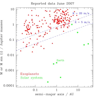
In Figure 1.13 we show a plot of planet minimum mass against orbital semi-major axis for ra-dial velocity planets (red triangles) and solar system planets (green squares). Here the lower mass limits of the radial velocity method with current technology become very clear. At an accuracy of∼3 m s−1_{, which is the current limit, we can detect Jupiter and maybe Saturn, but other Solar}

system planets would be out of reach. Even though we may be able to improve on the accuracy of the radial velocity method with technological advancements, there may be a fundamental limit to the radial velocity method in that stars can show a radial velocity jitter of up to∼20 m s−1

themselves which would hide any smaller planetary signal [95]. Radial velocity jitter is dependent on the stellar spectral type and activity level, and for G and F main sequence stars is generally less than 2 m s−1_.

1.8.3 Metal Rich Stars

(35)

[image:35.595.96.460.92.470.2]

Figure 1.13: Plot of minimum planet mass against semi-major axis for radial velocity planets (red triangles) and solar system planets (green squares). The dashed blue lines mark radial velocity curve semi-amplitudes of 20 m s−1 _{and 5 m s}−1_{. The plot was taken from the website by Phil}

Armitage in the reference [104].

metal content than our Sun). With the growing number of detected planets, this early trend was confirmed [71] and strengthened by a homogeneous metallicity determination for a set of planet-hosting and comparison stars [72]. The abundance ratios of “non-Iron” chemical elements in the stellar atmosphere ([Li/H], [C/H] and [N/H]) are found to be comparable for stars with and without planets [71],[72].

This observation fits in well with the idea that an abundance of heavier elements would favour planet formation. An intensive HST survey of the very metal poor globular cluster 47 Tuc ([Fe/H]

(36)

noted however, that in the case of 47 Tuc, the absence of planets could be due to the clusters high stellar density in the monitored region. Close stellar neighbours could prevent the formation of the protoplanetary disk. However, some debate of the theory has been made in the light of the discovery of a very old planet in the M4 globular cluster [82] since the stars in this cluster have a heavy element fraction that is 1/20th of the value for the Sun. Another scenario to explain the association of planets with metal rich stars is that the migration process which happens early on in the time of planet formation was without a braking mechanism and that many of the protoplanets ended their lives being engulfed by their parent stars [35].

D. Fischer & J. Valenti 2005 [23] analyse carefully the dependence of the probability of finding giant planets around stars as a function of metallicity. Figure 1.14 shows plots of the percentage of stars hosting a giant planet as a function of metallicity [Fe/H]. The data used to produce these plots consists of 850 stars for which radial velocity measurements have been made that would ensure the detection of planets with masses high enough to cause 30 m s−1 _{semi-amplitude radial}

velocity curves with periods of 4 years or less. It is very obvious that for stars with [Fe/H]<0.5, the probability of finding a giant planet is very small indeed, whereas for Solar metallicity this probability rises to∼3% and for [Fe/H]>0.3the probability is up to 15%. The relationship that they are able to derive from this data for the range−0.5<[Fe/H]<0.5is as follows:

P(Giant planet companion)= 0.03

NFe/NH

(NFe/NH)⊙ 2

(1.13)

Thus the probabilty of a star hosting a giant planet is proportional to the square of the number of iron atoms.

(37)

(a)

(b)

(38)

Design of the PASS0 Experiment

2.1 Introduction

This chapter is divided into two parts. The first part deals with the sources of observational noise for a charge-coupled-device (CCD) detector and the theory behind them. In the design of our experiment, we need to reduce the effects of the various noise sources as much as possible in order to reach the_∼1% precision required to detect planetary transits. The second part of the chapter is an introduction to the idea and design of PASS0, and the challenges that we face in order to get PASS0 to achieve its maximum precision.

2.2 CCD Signal and Noise Modelling

2.2.1 Readout Noise

On reading out a CCD pixel, noise is introduced into the signal from two sources:

1. The on-chip amplifier produces a statistical distribution of values centred on a mean value when converting from the analogue signal to a digital signal. Hence, even on reading out the same pixel twice with identical charge, a slightly different digital answer may be produced.

2. The output electronics themselves introduce spurious electrons into the readout process, producing unwanted random fluctuations in the output signal.

The readout noise, generally denoted byσRON, generally follows a Normal distribution. Hence it is quoted as a one-sigma value in electrons. It can be measured as the standard deviation of a bias frame, where a bias frame is a zero-second exposure with the shutter closed. The readout noise for the PASS0 camera with the Apogee U10 CCD is∼9 e−

(see Section 2.3.10).

2.2.2 Bias Level

The readout electronics apply a non-zero voltage to the CCD and the consequence of this is that on readout, the pixel values include an additive bias level. This bias level can vary from image to

(39)

38 CHAPTER 2. DESIGN OF THE PASS0 EXPERIMENT

image and hence a few extra read cycles are performed before or after reading the real physical pixels in order to quantify this level. This area of the image is called the overscan region, and the mean of this area is an estimate of the bias level. Images without an overscan region can be corrected for bias level by taking bias frames interspersed between the actual observations. This is the tactic we use with the PASS0 CCD which does not possess an overscan region.

2.2.3 Bias Pattern

On some CCDs there is a fixed pattern in the bias frames which will need to be removed from the science images by subtraction of the pattern. The easiest way to do this is to construct a master bias frame by combining many bias images together using the median or mean, which results in a high S/N estimation of the bias pattern.

2.2.4 Dark Current

The electrons in the silicon of a CCD may be thermally agitated and freed, consequently to be collected in the potential well of a pixel. Hence these thermal electrons accumulate along with the signal to be measured, and constitute a dark current. Clearly the dark current is a strong function of CCD temperature, and can be minimised by cooling down the CCD as much as possible. The cooling system of the PASS0 camera for instance achieves a CCD temperature of -20◦

C, which strongly suppresses the dark current for the CCD, but is not enough cooling to reduce it to a negligible level.

Characterising the dark current of a CCD at a particular temperature can be done by integrating the CCD for a certain time (usually the same integration time as the science observations) with the shutter closed so as to only accumulate thermal electrons. A large number of dark images can be combined to create a masterdark image which can be scaled to each science image using the relative exposure times and subtracted, since dark current is an additive effect.

The presence of a dark current can also introduce extra Poisson noise from the random nature of the thermal electrons. The thermal noise is usually denoted byσTHand it is given by:

σTH=

p

D(x, y) ∆t (2.1)

whereD(x, y) is the number of thermal electrons generated per second as a function ofxandy

position on the CCD, and∆tis the exposure time.

2.2.5 Photons

When the shutter on a CCD is opened, photons arrive at the CCD and knock electrons from the silicon valence bands, which are subsequently collected in the potential wells of the pixels. Photons in CCD observations arrive from two sources, sky background emission and astronomical objects. Independent of the source of the photons, the photons arrive in a random manner with a Poisson distribution. Hence, for a pixel of sensitivityF receiving a flux ofXphotons per second,

XF photo-electrons per second are produced and the photon noiseσPHamounts to

√

X F ∆tin a

(40)

Each pixel in a CCD has a slightly different sensitivity to photons. This non-uniformity in de-tector sensitivity can be characterised by imaging a bright uniform source (like the twilight sky). These type of images are called flatfields, and they may be combined, usually via the median to avoid bright stars, into a high signal-to-noise master flatfield which maps the sensitivity varia-tions. The master flatfield, after appropriate normalisation, is then used to correct the non-uniform sensitivity by dividing it into the science images.

The model for a raw CCD pixel valueZ(x, y)in electrons, taking into account all of the above sources, may be written as:

Z(x, y) =B(x, y) +D(x, y) ∆t+X(x, y)F(x, y) ∆t (2.2)

whereB(x, y)represents the bias pattern including the bias level (electrons),D(x, y)is the dark current per second,X(x, y)represents the distribution of incoming photons per second,F(x, y)is the master flatfield (dimensionless) and∆tis the exposure time in seconds. The calibrated CCD pixel valueX(x, y)in electrons per second is therefore given by:

X(x, y) = Z(x, y)−B(x, y)−D(x, y) ∆t

F(x, y) ∆t (2.3)

During the analogue to digital conversion in a CCD, electrons get converted to counts (or ADUs) at a rate ofGelectrons per ADU. The value ofGis referred to as the CCD gain. Equa-tions 2.2 and 2.3 can be used in either units of electrons or ADUs. The gain for the PASS0 camera with the Apogee U10 CCD is_∼2.3 e−

/ADU (see Section 2.3.10).

2.2.6 Pixel Noise

Combining all of the above discussion, we can write an expression for the noise in the raw pixel valueσZ in electrons as:

σ2_Z(x, y) =σ2_RON+σ2_TH+σ2_PH (2.4) All ofσRON,σTHandσPHhave units of electrons. Using the expressionsσTH =

p

D(x, y) ∆t

andσPH =

p

X(x, y) F(x, y) ∆tgives:

σ2_Z(x, y) =σ_RON2 +D(x, y) ∆t+X(x, y)F(x, y) ∆t (2.5)

Converting all quantities to ADU and ADU/s gives:

σ_Z2(x, y) =σ2_RON+D(x, y) ∆t

G +

X(x, y)F(x, y) ∆t

G (2.6)

The process of calibrating the CCD pixel values via Equation 2.3 affects the pixel noise model as follows:

σ2_X(x, y) = σ 2

RON

(F(x, y) ∆t)2 +

D(x, y)

F(x, y)2_G_∆_t+

X(x, y)

F(x, y)G∆t (2.7)

Again we are using ADU units in place of electrons (e−

), and ADU/s in place of e−

(41)

2.2.7 Measuring the CCD Gain

At this point we are in the position to be able to measure the CCD gain using Equation 2.7. The simplest way to do this is to take two consecutive and identically-exposed bias-corrected flatfields

F1 and F2 and form the difference image ∆F = F1 −F2. The exposure levelH of the two

flatfields can be measured by taking the mean of the central region. We are able to measure the noiseσ2

∆F(x, y) on the difference image, which is free from a flatfield pattern since it is the difference of two flat fields taken under exactly the same conditions. Assuming that the master flatfield is approximately 1 and that the dark noise is negligible, then we get:

G= 2H

σ2_∆_F(x, y)−2σ_RON2 (2.8)

This method may be repeated with numerous pairs of flatfields in order to get a set of gain mea-surements for the CCD from which the mean gain can be calculated. The gain for the PASS0 camera with the Apogee U10 CCD is∼2.3 e−

/ADU (see Section 2.3.10).

2.2.8 Signal-to-Noise Ratio

The photons from an astronomical source are rarely confined to a single pixel. The signal is spread over a small area of the CCD consisting of a group of pixels, and the distribution of the photons is defined by the combination of the source light distribution and the combined point-spread function (PSF) from the atmosphere and instrument. For stars, which are effectively point sources, the photons are simply distributed via the PSF.

If we assume that we have a signal ofN∗detected photo-electrons per second from a star, then

in ∆t seconds we obtain N∗∆tphoto-electrons on the CCD. These photo-electrons are spread

out overnpixpixels, which each contain a sky background signal ofNSKY∆tphoto-electrons. By assuming that the noise contribution from the dark current is negligible (for a low dark current), then the theoretical signal-to-noise (S/N) that we may get when measuringN∗∆tis:

S N =

N∗∆t q

N∗∆t+npix(NSKY∆t+σRON2 )

(2.9)

Note that hereσRONhas units of electrons, as in the rest of this subsection. This equation is called the “CCD Equation” [55], and there are various formulations of this equation in the literature (e.g., [58] and [29]).

We may rewrite Equation 2.9 for two cases when various noise sources dominate. Generally readout noise contributions never dominate sky noise contributions since there is always an appre-ciable sky background signal. In the case where the star is bright, and its photons dominate the sky photons,N∗∆t ≫ npixNSKY∆t, then we have:

S N =

p

N∗∆t (2.10)

(42)

0.1 1 10 100

0 20 40 60 80 100

Signal-To-Noise

Exposure Time (s)

N* = 1 e-/s, Nsky = 0 e-/s N* = 10 e-/s, Nsky = 0 e-/s N* = 100 e-/s, Nsky = 0 e-/s

Figure 2.1: Example plot of signal-to-noise versus exposure time for a star signal spread out over a 100 pixel area (regardless of shape). The various values forN∗ and NSKY are labelled on the different curves. All curves are proportional to√∆t. It is assumed that the CCD does not saturate.

then we have:

S N =N∗

s

∆t

npixNSKY

(2.11)

In both cases, the signal-to-noise of the star signal only grows as S/N ∝ √∆t. In Figure 2.1, we show the evolution of the signal-to-noise versus time for a set of stars with different fluxes and measured under different sky background conditions. Readout noise is considered negligible and saturation is ignored.

(43)

we find that:

∆t=−B+

p

(B2₋₄_AC₎

2A

A=N∗2

B =−(S/N)2(N∗+n_pixN_SKY) C =₋(S/N)2npixσ2RON

(2.12)

2.2.9 Lightcurve Noise

Here we derive the expected scatter in the lightcurves as a function of star brightness. These calculations are necessary because they help to define the theoretical best precision that we can reach in our lightcurves, in the case that we have a “perfect” data reduction pipeline. Since our pipeline will not be perfect, these calculations will allow us to assess the quality of our reductions. The result also depends on the method used to perform photometry on the calibrated CCD images. We get a different result for aperture photometry as opposed to optimal PSF scaling. We derive both results below.

We start by assuming that we have a CCD detector with readout noise σRON in ADU and gainG. We assume that the dark current is negligible so that D(x, y) _≈ 0, that the flatfield is

F(x, y) ≈ 1and we use a single exposure time of ∆tseconds. We represent the sky counts (ADU/s/pix) asS(t) wheret is the time of observation, and the star counts (ADU/s) byN∗(t).

Our pixel noise model then becomes (using Equation 2.7):

σ_X2(x, y, t) = σ 2

RON

∆t2 +

X(x, y, t)

G∆t (2.13)

whereX(x, y, t)andσX(x, y, t)represent the calibrated pixel value and its error bar (in units of ADU/s), as functions of pixel coordinatesxandy.

In aperture photometry, we measure the star flux by placing a circular aperture of radius R

pixels at the position of the star, summing the counts in this area and subtracting the sum of the sky counts in this area. The sky background level can be estimated using a larger annulus around the star aperture and calculating the median of these pixels (to protect from other objects contaminating the sky flux). The number of pixels in the star aperture is simplyπR2 pixels. To summarise this process in an equation we may write:

N∗(t) = X

x,y

X(x, y, t)₋πR2S(t) (2.14)

(44)

point-spread function. Using Equation 2.13, the variance ofN∗(t)is given by:

σ_N2_∗(t) =X

x,y

σ_X2(x, y, t)

=πR

2_σ2

RON

∆t2 +

πR2_S₍_t₎

G∆t +

N∗(t) G∆t

(2.15)

In astronomy we usually work in magnitudes, and we convert the flux to a magnitudem(t)via the relation:

m(t) =M0−2.5 log(N∗(t)) (2.16)

where M0 is some zeropoint magnitude. The zeropoint may vary from image to image, and is

usually determined from a set of standard stars in the field of view. The corresponding error bar onm(t), denoted byσm(t), is given by:

σm(t) = 1.0857σN∗(t)

N∗(t)

(2.17)

The root-mean-square (RMS) uncertainty in the mean level of a lightcurveσLCmay be calculated from:

σ_LC2 =

P

tσ2m(t)

NIM

(2.18)

whereNIMis the number of images in the sequence. By combining Equations 2.15, 2.17 and 2.18, we may derive:

σ_LC2 = 1.0857 2

NIM

πR2σ2_RON

∆t2

X

t

1

N∗(t)2

+ πR

2

G∆t X

t

S(t)

N∗(t)2

+ 1

G∆t X

t

1

N∗(t) !

(2.19)

In PSF photometry, we measure the star flux by fitting a PSF model at the position of the star. This PSF model is usually previously constructed from fits to suitable bright and isolated stars. Fits may be analytical, empirical or some combination. We consider the case where a known empirical PSF is simply scaled to the star at its already known position, and where the scaling is done using the optimal scaling formula. This case corresponds to the difference imaging pipeline we use to reduce our data later on (see Section 3.1). Since we are measuring difference images (see Sections 3.1.3 and 3.1.4), the flux we are measuring is a difference flux, which we denote as

∆f(t), with units ADU per second.

We represent the PSF as the functionP(x, y, t). Then, using the optimal scaling formula, we may measure∆f(t)as:

∆f(t) =

P

x,yX(x, y, t)P(x, y, t)/σX2 (x, y, t)

P

x,yP(x, y, t)2/σX2 (x, y, t)

(2.20)

The associated variance is given by:

σ_∆2_f(t) = P 1

x,yP(x, y, t)2/σ2X(x, y, t)

(45)

Figure 2.2: A diagram showing the design concept of the PASS instrument

Note that again, σ2

X(x, y, t) is given in Equation 2.13 as our pixel noise model. In difference imaging, the total star fluxN∗(t)may be obtained from the following equation (see Section 3.1.4):

N∗(t) =Fref+

∆f(t)

p(t) (2.22)

whereFref is the star flux as measured on the reference image in ADU/s (see Section 3.1.2, and

p(t)is the photometric scalefactor (see Section 3.1.4). Therefore the error onN∗(t)is given by:

σ_N2

∗(t) =

1

p(t)2P

x,yP(x, y, t)2/σX2 (x, y, t)

= σ

2

∆f(t)

p(t)2 (2.23)

To calculate the final noise in the lightcurveσLC, we need to use Equations 2.17 and 2.18. There is no simple analytical expression forσLCas in the aperture photometry case.

2.3 PASS: Permanent All Sky Survey

2.3.1 The Motivation and Ideas Behind PASS

The primary goal and original envisioned idea of the Permanent All Sky Survey (PASS) is to detect all transiting hot Jupiters in the entire sky, complete for host stars between 5.5-10.5 mag, with transits deeper than∼10 mmag, and with periods up to 1 week [20]. To achieve all-sky coverage, at least two sites are required, and so we consider here how the experiment would be set up at a single site. The sky above 30◦

(46)

of short focal length (approximately 50 mm and f-ratio f/1.4) orientated in different directions. The CCD cameras would be fixed on a sturdy platform, ensuring the mechanical stability and simplicity of the instrument, and a completely removable enclosure would be used to protect the instrument when not in use. Figure 2.2 shows how PASS might look in reality.

One key in the design of PASS would be the synchronization of the start of each exposure with Local Sidereal Time (LST). By ensuring that images are always taken at a fixed set of LSTs, stars will trail over exactly the same CCD pixels for a given LST on different nights. The resulting pho-tometry of stars at the same LST will then avoid systematic errors, such as flatfielding errors, that do not vary from night to night. Also groups of images from a single LST are directly comparable and already aligned with each other.

The data collected by PASS will not just be useful for planet hunting, but will also supply information about any variability in the field, whether they be variable stars, moving objects, or transient events. PASS will provide a temporal spacing of around 30 seconds between data points, allowing the characterisation of variable stars with periods as short as half an hour and as long as years, depending on the length of operation of PASS (which will hopefully be indefinite). Moving objects, such as asteroids, will drift slowly through the field of view, and astrometry and photometry can be performed on such objects. Transient events may appear in just one image, but the all sky coverage and high duty cycle will ensure the observation of events brighter than_∼10th magnitude.

PASS is not the first project to attempt all-sky surveillance. The All Sky Automated Survey (ASAS; [64]) observes the whole southern sky once every two days, and provides reliable pho-tometry down to_∼14 mag. This survey has published the discovery of many variable stars (e.g, [65], [66]). The RAPTOR survey [91] is a spatially distributed system of autonomous robotic telescopes that is designed to monitor the sky for optical transients. The Kilodegree Extremely Little Telescope (KELT; [60]) is a survey for planetary transits of bright stars (8-10 mag) using a small-aperture wide-field (26◦

x26◦

) robotic telescope. The camera achieves coverage of∼25% of the northern sky by cycling through a fixed set of observation fields. The project has produced∼4 transit candidates [61], none of which have been proven to be planets. Finally, it should be noted that there has already been one transit detection experiment similar in design to PASS. This was the South Pole Exoplanet Transit Search [13] that uses a large-format CCD and a fast f/1.5 300 mm focal length lens to give a seven degree field-of-view. No results have been reported to date.

2.3.2 PASS0: A Prototype PASS Experiment

Our prototype PASS experiment, which we name PASS0, was constructed with a single CCD and lens combination. The aim of PASS0 was to test the ideas behind the PASS experiment. Our first task was to evaluate the CCD detector and lens combination that would be used, and compare it to that used by the SuperWASP experiment.

(47)

For each CCD we are given information by the manufacturer on quantum efficiency (QE), the size/dimensions of the CCD in pixels and the pixel size in microns. This information is listed in Table 2.1 for the CCDs that we have chosen to evaluate. We also list in the table the focal length of each lens used in the evaluation, along with its maximum aperture. We proceed to evaluate the CCD and lens combinations by calculating the following quantities using the recipe we describe below.

To calculate the pixel size in arcseconds∆arc, we use the relation:

∆arc =

3600×180

1000×π

× ∆µ fl (2.24)

where∆µis the pixel size in microns andflis the focal length of the lens in mm. The field-of-view, FOV, in degrees of each camera is given by:

FOV=p

DxDy×

∆arc

3600 (2.25)

whereDxis the CCD size in thex-direction in pixels, andDy is the CCD size in they-direction in pixels. However, for PASS0, where stars trail across the CCD, this FOV would need scaling according to how long it takes for a star to trail across the CCD and the length of an observing night. For simplicity we do not make this adjustment, especially since we are trying to compare various CCD and lens combinations. To calculate the sky magnitudeMSKY, assuming a standard sky magnitude per square arcsecond of 18, and assuming a typical FWHM of 2 pixels for the PSF, we use:

MSKY= 18−2.5 log(A)

A=Neff∆2arc

=

π

2 ln(2)

×4 ∆2_arc

(2.26)

whereNeff is the number of effective pixels of a Gaussian PSF. To get this result we have used Equation B.8 from the Appendix B.

(48)

magnitude point source object as:

Vcps= 106×Q×

π

4

×D2_l

Dl=

fl

10fs

(2.27)

whereQis the detector quantum efficiency,Dlis the lens diameter in cm andfsis the lens f-stop. The counts per second due to sky backgroundScpsare then calculated via:

Scps=Vcps×10

−₀_.₄_M_SKY

(2.28)

and the number of sky counts received during the transit durationST is then given by:

ST =ScpstT (2.29)

wheretTis the transit duration in seconds. In a similar way we can derive:

CT=Vcps×10−0.4M∗×tT (2.30)

whereCT is the star counts during one transit. Using Equation 2.9 (ignoring readout noise), we get the signal-to-noise for one transit SNR1as:

SNR1 =

CT

√

CT+ST

δT (2.31)

whereδT is the fractional transit depth. For more than one observed transit we derive a signal-to-noise SNRN given by:

SNRN =SNR1

√

N (2.32)

whereN is the number of observed transits. Our requirement is that we can detect multiple transits at a SNR of 10. We can rearrange Equations 2.30, 2.31 and 2.32 to get a quadratic equation for the number of star counts during one transit:

C_T2−B2CT−B2ST= 0 (2.33)

B = SNRN

δT

√

N (2.34)

The quadratic equation can be solved in the standard way and we take the positive solution to get:

CT =

B 2 ×

B+pB2_{+ 4}_S

T

(2.35)

Finally, the faint star limit for a SNR of 10 is calculated from:

M∗ =−2.5 log

CT

VcpstT

(49)

4 8 C H A P T E R 2 . D E S IG N O F T H E P A S S 0 E X P E R IM E N T

Table 2.1: Evaluation of each CCD and lens combination, listing useful quantities to be taken into account when designing the survey.

CCD Lens QE Dimensions Pixel Size Pixel Size FOV Sky Faint Star Distance Number Of Planet Discoveries (pixel) (micron) (arcsec) (deg) Magnitude Magnitude Limit (pc) Stars (×103

) Per Month AP47P 35mm, f/1.4 0.7 1024x1024 13.3 78.4 22.3 6.14 9.08 75 1.07 0.55