Impacts of dynamic interactions on the predicted thermal performance of earth–air heat exchangers for preheating, cooling and ventilation of buildings

(1)

. . . .

Impacts of dynamic interactions on the

predicted thermal performance of earth – air

heat exchangers for preheating, cooling and

ventilation of buildings

Guohui Gan

*

Department of Architecture and Built Environment, University of Nottingham,

University Park, Nottingham NG7 2RD, UK

*Corresponding author: guohui.gan@nottingham.ac. uk

Abstract

Earth – air tunnel ventilation is an energy efficient ventilation technique that makes use of relatively stable soil temperature in shallow ground for preheating and cooling of supply air to a building. During operation, an earth – air heat exchanger interacts with the soil and atmosphere and the performance varies with the soil and atmospheric conditions. A computer program has been developed for modelling of coupled heat and moisture transfer in soil and for simulation of the dynamic thermal performance of an earth – air heat exchanger for preheating and cooling of a building. The impacts of dynamic interactions between the heat exchanger, soil and atmosphere are illustrated from the comparison of the heat transfer rate, heat exchanger temperature and supply air temperature through the heat exchanger for both preheating and cooling. It is shown that neglecting the interactions between the heat exchanger, soil and supply air would over predict the thermal performance of an earth – air heat exchanger. Neglecting the interactions between the soil surface and atmosphere while assuming axi-symmetric distributions of heat and moisture transfer as well as soil properties around the heat exchanger is not only unrealistic but also would fail to produce reliable data for long-term operational performance of the earth – air heat exchanger installed in shallow ground. The performance of an earth – air tunnel ventilation system can be enhanced when operated for both winter preheating and summer cooling of a building.

Keywords:earth – air heat exchanger; heating and cooling; building ventilation; heat transfer; moisture transfer; dynamic interaction

Received 27 August 2015; revised 21 October 2015; accepted 24 October 2015

1 INTRODUCTION

Earth – air tunnel ventilation is an energy-efficient approach to preheat or cool supply air to a building through a ground or earth – air heat exchanger. The heat exchanger consists of a series of pipes or ducts buried in shallow ground for transferring heat between the supply air in the pipes and the surrounding soil with a relatively stable temperature.

The performance of earth – air heat exchangers can be as-sessed analytically, numerically or experimentally. Analytical techniques are generally based on the simplified solution of one-dimensional (axi-symmetric) heat transfer in a circular pipe or the surrounding soil of homogeneous properties [1 – 3]. Such techniques have been incorporated into computer programs for

building performance simulation including TRNSYS by Al-Ajmi

et al.[4] and EnergyPlus by Lee and Strand [5] to investigate the potential of earth – air heat exchangers. Sanusi et al. [6] used EnergyPlus to assess the effects of the climate, soil and pipe on the cooling potential of an earth – air heat exchanger in hot and humid climates, in addition to conducting field measurements of its performance. The analytical models are simple and can generate data quickly for system performance evaluation or optimal system design in terms of thermodynamic and econom-ic performance [7]. However, in earth – air tunnel ventilation, heat and moisture transfer occurs simultaneously and varies in time and space due to the influence of daily and seasonal climat-ic variations and interactions between soil and the heat exchan-ger. An analytical technique would not be able to provide

International Journal of Low-Carbon Technologies 2015, 0, 1– 16

#_{The Author 2015. Published by Oxford University Press.}

This is an Open Access article distributed under the terms of the Creative Commons Attribution Non-Commercial License (http://creativecommons.org/licenses/ by-nc/4.0/), which permits non-commercial re-use, distribution, and reproduction in any medium, provided the original work is properly cited.

at University of Nottingham on November 25, 2015

http://ijlct.oxfordjournals.org/

(2)

accurate solution for multi-dimensional heat transfer or coupled heat and moisture transfer. For example, results from an analy-tical model would indicate that the air temperature inside a hori-zontal heat exchanger varies linearly along the pipe [5] because the model does not take account of horizontal variations in soil properties and heat transfer whereas measurement and multi-dimensional simulation would show that the variation of the air temperature is nonlinear. The solution of three-dimensional transport problems requires a numerical method. A numerical model can be for heat transfer only [8 – 12] or for simultaneous heat and moisture transfer [13 – 18]. Most numerical models involving coupled heat and moisture transfer have made use of simplifications such as symmetry around a horizontal axis for part of the computational domain. Some models even neglect the heat transfer between soil and atmosphere by simplifying the soil surface temperature to be the same as air temperature [12] or ignore the influence of atmosphere completely using an axi-symmetric model for the whole domain [11].

The author recently developed a more general three-dimensional numerical model for the simulation of transient heat and moisture transfer in soil with a horizontally coupled earth – air heat exchanger for preheating and cooling of buildings [19]. The model included all the principal interactions of heat and moisture transfer in soil and between the atmosphere, soil, heat exchanger and supply air passing through the heat exchan-ger. It was then used to investigate the potential of earth – air heat exchangers for preheating supply air in the UK conditions and compare the results with those from a simplified analytical model for soil temperature and an axi-symmetric model for the whole computational domain [20]. Results from the simpli-fied models were found to differ significantly from the general numerical model. The numerical model has been used for further simulation of the performance of earth – air heat exchan-gers for both preheating and cooling of supply air in building ventilation. In this paper, results using the model are presented. Emphasis is placed on the impacts of the interactions on the predicted performance in terms of the amount and rate of heat transfer and the temperatures of the heat exchanger and supply air.

2 METHODOLOGY

To simulate transient thermal performance of an earth – air heat exchanger, a numerical method is used to solve a system of equa-tions for three-dimensional heat and moisture transfer in soil together with initial and boundary conditions.

2.1 Model equations

The following coupled energy and mass conservation equations describe the three-dimensional transient heat and moisture transfer in soil with phase change:

@ðrCTÞ

@t ¼ rððkþLrlDT;vÞrTÞ þ rðLrlDQ;vrQÞ þqv ð1Þ

@Q

@t ¼ rððDT;lþDT;vÞrTÞ þ rððDQ;lþDQ;vÞrQÞ þ

@K

@z þQv ð2Þ

where C denotes specific heat of soil (J/kgK); DT,l represents thermal liquid diffusivities (m2/sK); DT,v represents vapour moisture diffusivities (m2/sK); DQ,l denotes isothermal liquid diffusivities (m2/s);DQ,vrepresents isothermal vapour moisture diffusivities (m2/s); Krepresents hydraulic conductivity of soil (m/s); k represents thermal conductivity of soil (W/mK); L

represents latent heat of vaporisation or fusion of water (J/kg);

qvrepresents volumetric heat production/dissipation rate in soil (W/m3); Tdenotes temperature of a medium (soil) (8C); ris density of soil (kg/m3);rlis density of liquid (kg/m3);Q repre-sents volumetric moisture content (m3/m3);Qvindicates source or sink of moisture in soil (m3/m3s);zis vertical coordinate (m).

Soil is a mixture of solid matter, gases and liquids as well as living organisms. The key thermal properties of a soil mixture that influence heat and moisture transfer are the density, specific heat and thermal conductivity, which are calculated using the following functions of the volumetric composition of dry solid matter, gases and three phases of moisture—liquid water, water vapour and solid ice:

r¼X n

m¼1

rmumþrlulþriuiþrpup ð3Þ

C¼

Pn

m¼1rmCmumþrlClulþriCiuiþrpCpup

Pn

m¼1rmumþrlulþriuiþrpup

ð4Þ

k¼ Pn

m¼1 fmkmumþklulþ fikiuiþfpkpup Pn

m¼1 fmumþulþfiuiþfpup

ð5Þ

whereurepresents volumetric fraction of a constituent in soil;f

denotes ratio of the average temperature gradient of the soil constituent to that of water;

Subscript m is the mth component of n types of dry soil grains,lstands for liquid moisture,ifor ice andpfor gas-filled pores.

The partial differential equations (1) and (2) are solved for a three-dimensional model using the control volume method with the initial and boundary conditions described below.

2.2 Initial and boundary conditions

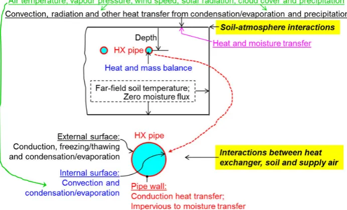
A heat exchanger is represented by a series of parallel pipes inside a computational domain. Boundary conditions for the solution of the three-dimensional heat and moisture transfer equations include heat and moisture transfer for the ground or top soil surface to account for the interactions between soil and atmosphere and the interior and exterior surfaces of the heat exchanger pipe to account for the interactions between the heat exchanger, soil and supply air as well as the bottom face, four vertical faces, the inlet and outlet openings for the

(3)

pipes. Figure 1 shows the boundary conditions on a vertical plane normal to the heat exchanger.

The following expression describes the annual variation of the soil temperature and is used to set the far-field (the domain faces far away from the heat exchanger) temperature at any time

t(day) and depth as well as the initial soil temperature,

T¼TmTampeZ=Dsin ðtt0Þ

2p

365

Z

D

p

2

ð6Þ

whereDrepresents damping depth of annual temperature fluc-tuation (m); Tamp indicates annual amplitude of soil surface temperature (8C); Tm indicates annual mean temperature of deep soil (8C);trepresents time (s);t0represents time lag from a starting date to the occurrence of the minimum temperature in a year (day);Zrepresents depth from soil surface (m).

Since such an expression is not available for moisture vari-ation in soil, the far-field moisture transfer is taken to be zero and the initial soil moisture content to be uniform.

The interactions between soil and atmosphere are represented by the following heat and mass balances for a control volume of top soil with a thickness ofdj:

ðkþLrlDT;vÞ @T

@jþLrlDQ;v

@Q

@j ¼qf ð7Þ

ðDT;lþDT;vÞ @T

@jþ ðDQ;lþDQ;vÞ

@Q

@j ¼Qf ð8Þ

whereqfis net heat flow into the control volume resulting from short and long wave radiation, natural convection due to com-bined wind and buoyancy effects, evaporation of moisture from or condensation to the ground surface and sensible heat from

precipitation (W/m2); Qfis the net mass flow into the control volume due to precipitation and evaporation or condensation of moisture;jis direction normal to a boundary.

The interactions between the heat exchanger, soil and supply air involve two areas of heat and mass transfer—the outer and inner surfaces of the heat exchanger pipe. For the outer surface, Equations (7) and (8) are also used but with zero source/sink for both heat and mass on the right hand side. For the inner surface, interactions between the surface and moving air account for the transient heat and moisture changes in supply air through con-duction, convection, evaporation or condensation and heat or moisture accumulation or dissipation. Heat transfer between the outer and inner surfaces of the solid pipe wall, which is impervi-ous to moisture transfer, is calculated using Equation (1) without the effect of phase change.

Further details of the boundary conditions are described in References [19, 21].

The conditions of supply air at the inlet opening of the heat exchanger are specified with ambient temperature, vapour pres-sure (or humidity) and ventilation rate (or mean velocity). At times when incoming air temperature is higher or lower than the pipe temperature such that preheating or cooling, respective-ly, of supply air is not possible, the inlet opening is prescribed with zero heat and mass flux for continuous simulation of heat and moisture transfer in soil and heat transfer in the pipe wall.

The numerical method is used to assess the performance of an earth – air heat exchanger for preheating and cooling of supply air in a climate in the Southern England, represented by operation in December and July, respectively, with the following specifications for the heat exchanger, soil and atmosphere:

[image:3.612.132.478.490.699.2]

† Heat exchanger: the heat exchanger is made of high-density polyethylene. Its external diameter is 200 mm and wall

Figure 1. Boundary conditions for simulation of heat and moisture transfer through an earth – air heat exchanger.

(4)

thickness is 7.7 mm. It is installed horizontally at 1.5 m below the ground surface. The mean velocity of supply air is 2 m/s at the inlet of the heat exchanger.

† Soil: the type of soil in consideration is of loam texture, which typically is composed of 43% sand, 18% clay and 39% silt [22]. Its saturation moisture content is 44% and residual moisture content is 5%. The initial moisture content is taken to be one half of the saturation value. The temperature of deep soil for the site is108C.

† Environmental properties: the climatic data for atmosphere are time dependent. The hourly data for air temperature, partial vapour pressure (or wet bulb temperature), solar radi-ation, cloud cover and wind speed for each month are taken from the CIBSE Guide [23]. The monthly rainfall is obtained from a weather station [24] with an assumption that it would rain for 3 h in evening on every third day based on the average rain days in a year.

The model has been validated for simulation of transient heat transfer for preheating of supply air through a heat exchanger of the same size and installation depth as described earlier [19, 20].

3 RESULTS AND DISCUSSION

Simulation has been carried out for preheating in December and precooling in July. Results are discussed in terms of the rate and/or amount of heat transfer, the temperature of the heat exchanger and the temperature of air at the outlet of the heat ex-changer. The magnitude of heat transfer through a heat exchan-ger is a principal indicator of its thermal performance whereas the two temperatures are included as additional criteria for assessing the impacts of the interactions at the interfaces.

3.1 Winter

preheating

Figure 2 shows the predicted daily variations in ambient air tem-perature and soil surface temtem-perature together with the tempera-ture of undisturbed soil at the same depth as the heat exchanger in December and soil temperature along a vertical line through the heat exchanger at the end of five typical days. The daily air temperature varies by 5.78C from the minimum of 20.18C in the early morning (3 am) to the maximum of 5.68C in the after-noon (3 pm) at the beginning of the month. The air temperature first decreases slightly till the middle of the month to a minimum and maximum of 20.48C and 4.98C, respectively, and then increases gradually to a minimum and maximum of 0.78C and 5.98C, respectively, at the end of the month. The daily variation of soil surface temperature is much larger because of radiation heat transfer. The source for the higher surface tem-perature than the ambient temtem-perature during the daytime is absorption of solar radiation whereas the lower surface tempera-ture during the night time is mainly a result of long wave radi-ation heat loss. The variradi-ation in the surface temperature would be even larger without natural convection, which decreases the surface temperature during the peak of the daytime but increases

in the night. The soil surface temperature drops below the freez-ing point durfreez-ing much of the night times. The minimum surface temperature is about 23.58C (between 4 am and 5 am) at the beginning of the month and drops to 24.88C in the fourth night. The overall trend of the minimum surface tem-perature is upward towards the end of the month, reaching

21.88C in the last night. The maximum surface temperature is 7.38C (between noon and 1 pm) at the beginning and increases to 8.78C on the third day and 9.58C near the end of the month. The rain in the proceeding night would decrease the soil surface temperature in the following 2 days due to the lower rainwater temperature and increased moisture evaporation. This can clearly be seen from its reduced maximum and minimum tem-peratures. It is worth pointing out that in their mathematical modelling of an earth – air heat exchanger, Haghighi and Maerefat [12] assumed the soil surface temperature to be the same as ambient air temperature. The results from the present study have however shown that the soil surface temperature differs significantly from air temperature at any time of a day due to the coupled heat and moisture transfer between the soil surface and atmosphere.

[image:4.612.328.552.57.330.2]

The temperature of the undisturbed soil at 1.5-m deep is 10.48C at the beginning of the month and decreases to 8.18C at the end of the month. It is higher than the ambient air tem-perature throughout the month. The soil temtem-perature above the heat exchanger is lower than the deep soil temperature and decreases with time. The vertical soil temperature variation is influenced by the heat exchanger in an area of only 0.6 m from

Figure 2. Predicted temperature variations in December. (a) Daily variations

in ambient air and soil surface temperatures, (b) vertical variation in soil temperature.

(5)

the pipe at the end of the first day. During the night time, the soil temperature decreases from heat transfer to the cold ambient at the ground surface while at any time of a day it would also decrease with operating time due to heat extraction through the heat exchanger when preheating is feasible. For simulation of preheating operation, heat transfer from soil to air through the heat exchanger takes place when the temperature of the heat exchanger at the inlet opening is higher than the air temperature. At the end of the month, the soil temperature sur-rounding the heat exchanger is only 58C compared with the undisturbed soil at the same depth of 88C. Meanwhile, the soil temperature above the heat exchanger is much lower than that below; the average temperature over a distance between the top surface and heat exchanger is 38C compared with 6.48C below the heat exchanger of the same distance.

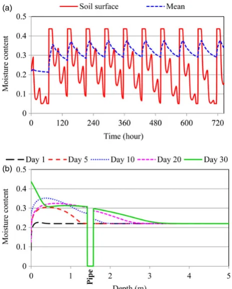
The daily variations of surface and mean moisture for the month and vertical variation in soil moisture are shown in Figure 3. The mean moisture is calculated for the soil layer between the soil surface and the crown of the pipe for the heat exchanger. Moisture evaporates from the soil during day times. As a result, the surface moisture would drop rapidly after the sun rises and reach the minimum value before sunset because the evaporation rate would be larger than the moisture transfer rate from soil below. Unlike in earlier months such as October when the soil surface could be dry during part of the daytime [19], the soil surface would not be so dry this month because of the lower air temperature and evaporation rate. During the evening and

onwards, the surface moisture would increase as a result of upward moisture transfer in soil and moisture condensation or frost formation when the surface temperature drops below the freezing point. The mean moisture for the soil layer would increase during the rainfall on every third evening and then decrease afterwards. Overall, the amount of rainfall and moisture condensa-tion exceeds that of surface evaporacondensa-tion during the first week. The variation pattern remains almost constant afterwards from a minimum of 29% to a maximum of 38% between a rain cycle.

In the depth direction, the overall trend of moisture variation is also increasing with time. At the end of the first day, the mois-ture variation is limited to the close vicinity of soil surface. The influence of moisture variation reaches 3.5 m below the soil surface at the end of the month and the soil moisture at the in-stallation depth increases to 30%.

The rate and amount of heat transfer through a heat exchanger and its temperature as well as the temperature rise of supply air and the outlet air temperature vary with the length. Simulations have been performed for the heat exchanger with different lengths from 10 to 40 m in addition to a unit length (1 m).

Figure 4 shows the predicted variations with time in the tem-perature of the inner pipe surface and heat transfer rate through one pipe of a 40-m-long heat exchanger, together with the ambient air temperature and the temperature of undisturbed soil at a depth of 1.5 m (denoted by soil temp) for reference, for heating in December. The variation in the mean temperature of the 40-m-long heat exchanger (defined as the average temperature of the inner surface of the pipe) is much less than that of the ambient air. The daily variation is0.78C compared with 5.78C for the ambient air.

[image:5.612.55.287.396.685.2]

The heat transfer rate per unit length of the heat exchanger varies with time and with soil and ambient temperatures. Because the soil temperature is more stable than air temperature, the heat transfer rate is higher during the night time when the air tempera-ture is much lower than that in the daytime. Generally, the vari-ation in the heat transfer rate follows inversely that of air temperature. The minimum and maximum values are observed at 3 am and 3 pm, respectively, for air temperature but 3 pm and 3 am, respectively, for the heat transfer rate. The heat transfer rate decreases day by day due to the decreasing soil temperature and from Day 19 the minimum value drops to zero between 1 pm and 3 pm when the air temperature becomes higher than the

Figure 3. Predicted moisture variations in December. (a) Daily variation, (b)

vertical variation.

Figure 4. Predicted variations with time of pipe temperature and heat transfer

rate for a 40-m-long heat exchanger in December.

[image:5.612.311.569.571.688.2]

(6)

temperature of the pipe at the inlet. This is defined to be the moment when heat in surrounding soil is not available for extrac-tion and preheating through the heat exchanger is supposed to stop by means of, e.g., by-passing supply air through the heat exchanger. The duration when heat extraction is not feasible increases with op-erating time from 2 h on Day 19 to 8 h on the last day of the month (from 10 am to 6 pm). The decrease in the soil temperature sur-rounding the heat exchanger results not only from the decreasing soil temperature at the installation depth but more importantly from the heat extraction through the heat exchanger. This can be seen from faster decreasing pipe temperature than the undisturbed soil temperature for the first 2 weeks of the month (Figure 4). The rate of decrease in the pipe temperature is smaller for the last week because the ambient air temperature begins to rise very slowly from the middle of the month but the rise accelerates in the last week.

The temperatures of soil, supply air and the heat exchanger and the heat transfer rate also vary horizontally and the varia-tions are nonlinear. As an example, Figure 5 shows the variavaria-tions in the pipe and air temperatures and heat transfer rate for a 40-m-long heat exchanger at the end (midnight) of Day 5. The air temperature increases along the heat exchanger from 0.68C at the inlet to 7.48C at the outlet because of heat transfer from soil to air. The pipe temperature also increases along the heat ex-changer but at a much smaller rate than air temperature from 5.28C to 8.48C. The temperature difference between the pipe and air (heating potential) is much larger near the entrance. The heat transfer rate decreases along the pipe from 22.8 W/m at the inlet to 5.3 W/m at the outlet. The magnitude of variations in the temperatures and heat transfer with the distance is depend-ent on the time as well as ambidepend-ent air and soil properties. The air and pipe temperatures and heat transfer rate along the heat exchanger at the end of Day 5 for example can be represented by the following quadratic correlations:

Ta¼ 0:003x2þ0:29xþ0:65 ðR2¼0:9994Þ ð9Þ

Ts¼ 0:0014x2þ0:14xþ5:1 ðR2¼0:9996Þ ð10Þ

q¼0:0082x20:75xþ22:3 ðR2¼0:9988Þ ð11Þ

where qrepresents heat transfer rate per unit length of heat ex-changer (W/m);Tadenotes air temperature in the heat exchanger (8C);Tsdenotes the temperature of the inner surface of the pipe (8C);xrepresents the horizontal distance from pipe inlet (m).

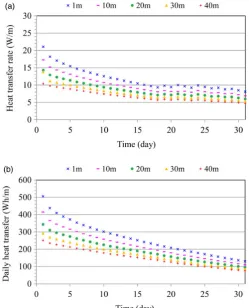
[image:6.612.316.566.375.684.2]

The results for the instantaneous heat transfer are used to cal-culate the daily mean values—the amount of daily heat transfer and mean rate of daily heat transfer. The amount of daily heat transfer is the cumulative product of the heat transfer rate and time for the duration of operating period when heat is available for extraction for heating (or injection for cooling) and the mean rate of daily heat transfer or daily mean heat transfer rate is the average of the heat transfer rate for the duration. The amount of daily heat extraction decreases continuously. The daily mean heat transfer rate decreases with operating time up to Day 18 and the decrease becomes negligible afterwards as shown in Figure 6. The negligible change of the daily heat transfer rate from Day 19 results from the way the average value is calcu-lated—it excludes part of the daytime with no heat transfer but for the preceding days the calculation includes the low heat transfer rate in the period; it is not because the daily variation pattern of the instantaneous value becomes stable, which decreases daily for the whole month as seen from Figure 4. The daily mean heat transfer rate (W/m) and the amount of daily heat transfer (Wh/m) also decrease with increasing length. The total heat transfer rate (W) is the product of the mean heat

Figure 5. Predicted variations of supply air and pipe temperatures and heat

[image:6.612.47.297.465.689.2]

transfer rate along the pipe length at the end of Day 5.

Figure 6. Predicted variations of heat transfer with time for different heat

exchanger lengths. (a) Daily mean heat transfer rate, (b) daily heat transfer.

(7)

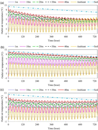
transfer rate and the pipe length, and this would however increase with length. As a result, the temperature of air flowing out of the heat exchanger (Figure 7) would depend on the pipe length as well as the ambient air temperature. It is seen from Figure 7a that a 10-m-long pipe would be able to reduce the daily temperature swing of supply air at the pipe outlet by one-third, a 20-m-long pipe by two thirds and a 30-m-long pipe by four fifths. A 40-m-long pipe would maintain the daily supply air temperature almost at a stable level with a variation of ,1/10 of the diurnal ambient air temperature swing (0.4–0.58C compared with 5.78C).

Heat transfer through the heat exchanger and the pipe and outlet air temperatures are influenced by the interactions between the heat exchanger, soil and atmosphere. The effects are assessed according to the interactions at the two areas of

interfaces: (a) between the pipe and soil at the outside surface of the pipe and between the pipe and supply air inside the pipe; (b) between soil and atmosphere at the ground surface.

3.1.1 Effect of interactions between the heat exchanger, soil and supply air

[image:7.612.137.474.242.687.2]

Analytical expressions for annual soil temperature variation such as Equation (6) indirectly and partially take into consideration of the influence of varying atmospheric conditions. These equations are derived for a soil mixture of uniform properties and without any heat transfer devices in soil such as a ground heat exchanger. Consequently, they cannot account for the influence on the soil surface from additional heat and mass transfer in soil with such a device and thus include only part of the interactions at the

Figure 7. Predicted outlet air temperature for different heat exchanger lengths using three methods. (a) With interactions between the heat exchanger and environments, (b)

with Equation (6) for soil temperature, (c) with axi-symmetric model.

(8)

surface. They are not able to take account of the history of heat transfer between soil and fluid through a heat exchanger either, which can alter the temperatures of both soil and the heat exchan-ger for heating (heat extraction) or cooling (heat injection) oper-ation. Equation (6) in place of Equation (1) is used to calculate the soil temperature at the pipe location as a means for assessing the effect of the interactions between the heat exchanger, soil and supply air. Similar analytical equations have been used by some previous investigators [2, 3].

Using Equation (6) for the soil temperature, the predicted heat transfer rate would be much higher than that predicted with consideration of all the thermal and moisture interactions at both interfaces. Figure 8 shows that neglecting the interactions between the pipe, soil and supply air increases the predicted in-terior pipe surface temperature but decreases its daily variation during preheating. The daily pipe temperature swing for a 10-m-long heat exchanger without considering the interactions is only 0.58C compared with 1.38C with interactions. The difference between the two temperature values with and without consider-ation of the interactions varies all the time each day but overall increases with operating time for the first half of the month. The difference stabilises in the third week and then decreases in the last week; the maximum differences occur on Day 20 with the maximum of 109% in the early morning (at 4 am to 5 am) and the minimum of 66% in the late afternoon (at 5 pm) at

resumption of heat extraction after the soil temperature recovery period from noon when air temperature is higher than the pipe temperature. Figure 8 also indicates that the difference in the pre-dicted heat transfer rate using the two methods (one with and the other without consideration of the interactions) increases with operating time and is larger than that in the temperature. The minimum difference in the heat transfer rate generally occurs at night between 1 am and 2 am. The difference would be much larger at other times particularly when the air temperature approaches the pipe temperature, leading to negligible heat trans-fer, during part of the daytime from Day 19 and hence there would be no preheating in the daytime for simulation with con-sideration of the interactions whereas simulation without consid-ering the interactions would indicate as if heat could be extracted all day long for the whole month. The highest minimum differ-ence in the heat transfer rate is 112% in the last day.

[image:8.612.321.557.367.678.2]

Figure 9 shows that the difference also increases with time in the amount or rate of daily heat transfer predicted with the two methods. The difference in the predicted daily heat extraction is larger than that in the heat transfer rate from the day when heat begins to ‘run out’ for extraction during a short period of daytime. The larger amount of daily heat transfer without con-sidering the interactions results not only from the predicted higher heat transfer rate but also from the longer time period for heating of supply air—continuous heating for the whole month

Figure 8. Effect of interactions on the predicted variation in pipe temperature

and heat transfer rate for a 10-m long heat exchanger. (a) Pipe temperature, (b) heat transfer rate.

Figure 9. Effect of interactions on the predicted variation in daily heat transfer

through a 10-m-long heat exchanger. (a) Daily mean heat transfer rate, (b) daily heat transfer.

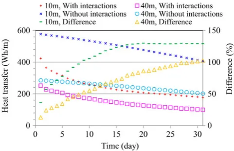
[image:8.612.49.297.374.676.2]

(9)

compared with 18 days from the beginning with consideration of the interactions. Note that the presented daily variation in the heat transfer rate from Day 19 is not smooth because the simu-lated results were recorded hourly for post-processing but the exact period when heat is available for extraction would vary from day to day by a fraction of the time. When the same period for heat extraction, i.e., from 8 pm to 9 am, is used for process-ing, the variation becomes smooth as is also shown in Figure 9a. With regard to the magnitude of the difference in the predicted heat transfer using the two methods, for the last day of the month, for example, the predicted daily heat extraction through a 10-m-long heat exchanger without considering the interac-tions is 231% higher than that with full interacinterac-tions compared with the difference of 170% in the heat transfer rate. The same patterns of variation in the heat transfer with time hold for longer heat exchangers but the differences decrease with increas-ing length. The differences in the amount and rate of heat trans-fer for a 40-m-long heat exchanger decrease to 139% and 95%, respectively, for the last day of the month.

The degree of the interactions between the heat exchanger and the surrounding soil and atmosphere also varies along the air flow direction in the heat exchanger. These interactions lead to the increases in air and pipe temperatures but decrease in the heat transfer rate along the heat exchanger. Because Equation (6) only accounts for the vertical variation in the soil temperature, the predicted variation in the pipe temperature along the heat exchanger is smaller but the variation in the air temperature is larger as indicated in Figure 5. Also, the heat transfer rate without considering the interactions is higher compared with the prediction with the interactions for the first half of the pipe length, but the decrease in the heat transfer rate along the heat exchanger is larger without considering the interactions. As a result, at the end of Day 5, after air travels horizontally for 22 m through the 40-m-long heat exchanger, the heating po-tential and heat transfer rate without considering the interac-tions become smaller than those with the interacinterac-tions. However, the mean heat transfer rate for the whole pipe is still larger without considering the interactions than that with the interac-tions, e.g., 14.8 W/m compared with 11.7 W/m at the end of Day 5. The position where the two lines for the heat transfer rate with or without considering the interactions intercept, i.e., 22 m from the inlet at the end of Day 5 in Figure 5, moves towards the downstream as the operation continues. For example, at the end of the month, the point of intersection is 6 m away from the outlet of the 40-m pipe. The mean heat transfer rate for the whole pipe is by then about two thirds larger without consider-ing the interactions (10.6 W/m) than that with the interactions (6.2 W/m).

[image:9.612.330.552.557.689.2]

As discussed earlier, the undisturbed soil temperature is higher than air temperature for the whole month such that pre-heating of supply air would be possible if the interactions between the heat exchanger, soil and ambient environments were not taken into consideration. By comparing Figure 7b with Figure 7a, it is seen that using Equation (6) instead of (1) the supply air could be predicted to reach a much higher

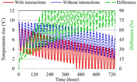
temperature and that a 40-m-long heat exchanger could have maintained a nearly constant supply air temperature with a devi-ation from the undisturbed stable soil temperature of only 0.68C at maximum. However, due to the interactions, the real soil tem-perature near the heat exchanger would decrease and the achiev-able supply air temperature would be lower, e.g., it is 4.78C in the early morning of the last day from the prediction with con-sideration of the interactions compared with 7.58C predicted without considering the interactions. Figure 10 shows the air temperature rise, i.e., the temperature difference between supply air at the pipe outlet and ambient air, through a 40-m-long pipe predicted with and without considering the interactions. It is seen that the error or the difference between the predictions using the two methods would increase with operating time. In the last day, the (minimum) difference at 3 am is 67% and the average difference for the operating period is 121%. In other words, neglecting the interactions would over predict the supply air temperature rise through a 40-m-long pipe significantly and the level of over-prediction increases with operating time, by at least two thirds at the end of the month.

3.1.2 Effect of interactions between soil and atmosphere

A pure axi-symmetric model has recently been implemented by some researchers [11] with the help of commercial fluid flow software to study the heat transfer and air flow through an earth – air heat exchanger. This type of model was used in the past to investigate the performance of ground heat exchangers when computers were not powerful enough to carry out three-dimensional modelling. The difference between the past and recent approaches to implement the model is that the original axi-symmetric model was a simplified representation of heat transfer in the vicinity of the heat exchanger installed in shallow ground but was linked somehow to the atmospheric conditions at the top soil whereas the pure axi-symmetric model completely neglected the interactions between soil and atmosphere as well as spatial variations in thermal and physical properties of soil. By the way, taking the soil surface temperature to be the air tem-perature [12] would have similar consequence to neglecting the interactions between soil and atmosphere.

Figure 10. Predicted variation with time in the temperature increase of supply

air through a 40-m-long heat exchanger.

(10)

To investigate the effect of neglecting the interactions between soil and atmosphere, simulation using the equivalent axi-symmetric model has also been conducted where the initial soil temperature is set to be uniform as the deep soil temperature (108C, which is incidentally close to the soil temperature at the installation depth at the beginning of the month (10.48C) and average temperature of undisturbed soil at the same depth for the whole month (9.28C)) and the heat and moisture transfer at the soil surface as well as far-field soil boundary is taken to be zero. Meanwhile the heat exchanger is positioned at a great depth such that there would be no heat transfer across the boundary for the period of operation investigated. Figure 11 shows that the variation with operating time in the heat transfer rate predicted with the axi-symmetric model is much less than that predicted with full interactions because the axi-symmetric model ignores the fact that the soil temperature is decreasing rapidly during the period. The heat transfer rate predicted with the axi-symmetric model is close to that predicted with full interactions for the first week or so because the soil temperature at the start is similar to the initial value given by Equation (6). Afterwards, however, the axi-symmetric model gives rise to higher heat transfer and the difference between the two models increases with operating time continuously. Besides, the percent-age difference between the predictions does not vary significantly with the length of the heat exchanger, increasing from under-prediction by 3% at the beginning to over-under-prediction by 65% and 70% at the end of the month for the 10- and 40-m-long heat exchangers, respectively. Compared with the predictions using Equation (6) for the soil temperature, which includes indirectly the influence of varying atmospheric conditions but takes no account of the interactions between soil and the heat exchanger (Figure 9), the axi-symmetric model would produce better results for this month. For other times, however, when the soil tempera-ture at the installation depth differs appreciably from the deep soil temperature such as in January, the axi-symmetric model would produce worse results [20]. Also, if simulation continues beyond the period of one month as that would be needed for winter heating, the over-prediction by the axi-symmetric model would

increase further and so much so that it would produce worse results from certain time onwards.

Figure 12 indicates that the predicted outlet air temperature using the axi-symmetric model is slightly lower than that with consideration of the interactions for the first 3 days because of the slightly lower value for the initial soil temperature (108C compared with 10.48C). The temperature from the axi-symmetric model is higher afterwards and for the second half of the month the daily variation pattern is almost independent of the time because the model could not take account of soil tem-perature variation. Thus, the differences in the temtem-peratures using the two methods also increase with operating time. As a result, the axi-symmetric model would not be able to predict the temperature of supply air in trend or magnitude for indoor thermal control, system design or evaluation of the long-term operational performance of an earth – air heat exchanger. In add-ition, from mathematics and physics points of view, the model is not appropriate because the distribution of soil temperature or moisture in vertical direction is far from axi-symmetric as seen from the examples in Figure 2b and Figure 3b. Even though the model might occasionally produce similar results to those from reliable sources, it is of more coincidence than science.

3.2 Summer precooling

Figure 13 shows the predicted variations with time in the tem-perature of the inner pipe surface and heat transfer rate through a 40-m-long heat exchanger as well as the ambient air tempera-ture and the temperatempera-ture of undisturbed soil at a depth of 1.5 m for precooling in July. The temperature of the undisturbed soil at 1.5 m deep is 11.98C at the beginning of the month and increases to 13.78C at the end of the month. It is much lower than the air temperature during day time for the month and also lower for most of the night time. Hence, there is a large potential for natural earth – air cooling.

[image:10.612.53.288.535.690.2]

The variation in the mean temperature of the long heat ex-changer is again much less than that of the ambient air. The daily variation is 1.88C at the beginning of the month when the ambient air temperature varies by 12.98C. The variation in

Figure 12. Comparison of the predicted outlet air temperature for a 40-m-long

heat exchanger.

Figure 11. Comparison of the daily mean heat transfer rate from 8 pm to 9 am

predicted with full interactions and with the axi-symmetric model.

[image:10.612.320.557.549.687.2]

(11)

the pipe temperature decreases to 0.98C compared with that in air temperature of 12.28C at the end of the month.

The heat transfer rate (cooling capacity for precooling oper-ation) is higher during the daytime when the air temperature is much higher than the soil temperature. It increases with air tem-perature in the morning until at3 pm and then decreases. The maximum heat transfer rate is 19.8 W/m at 3 pm of the second day and decreases to 11.5 W/m at the same time of the last day of the month. The rate of heat transfer would decrease day by day due to increasing soil temperature, which results from heat absorption from supply air in the preceding days and a slight in-crease of soil temperature with time that occurs naturally. Because of the heat absorption, the pipe temperature in the night time could become higher than the air temperature and natural cooling is then not feasible. Similar to the simulation for preheating, for precooling operation heat transfers from air to soil at any time of a day when the air temperature is higher than the temperature of the heat exchanger at the inlet opening. The duration when natural cooling of air by soil is not available increases with operating time from 4 h between midnight and 4 am on the second day to 11 h between 9 pm and 8 am on the last day of the month.

[image:11.612.139.476.59.210.2]

3.2.1 Effect of interactions between the heat exchanger, soil and supply air

Figure 14 shows that using Equation (6) for soil temperature at the depth of the heat exchanger, the predicted interior pipe surface temperature is lower and its daily variation much less than those with thermal and moisture interactions between the 40-m-long pipe and soil. The daily pipe temperature swing is only 0.78C compared with 1.88C in the early days to 0.98C near the end of month with consideration of the interactions. Consequently, the difference between the two temperature values with and without consideration of the interactions varies with operating time; the maximum differences occur on Day 20 with a minimum of 20.3% in the early morning (at 7 am) just before the beginning of cooling of supply air after the soil tem-perature recovery period in the night time when the air tempera-ture is lower than the pipe temperatempera-ture and a maximum of

23.6% in the late afternoon (at around 6 pm) near the end of heat injection session.

Because of the much lower soil and pipe temperatures, the heat transfer rate predicted with the fixed patterns of variation in soil temperature (Equation 6) for July is significantly higher than that with the interactions between soil and the heat exchan-ger as shown in Figure 15. As pointed out earlier, natural cooling would not be feasible during part of the night time when the interactions between the heat exchanger, soil and atmosphere are taken into consideration. Ignoring the interactions, however, would lead to a lower soil temperature than air temperature and thus would indicate a cooling potential for supply air all day long for20 days. As a result, depending on the length of heat exchanger, the difference between the predictions with and without considering the interactions would increase with time up to Day 20 for short heat exchangers. The difference in the daily heat transfer reaches a maximum of 130% on Day 20 for a 10-m-long heat exchanger. For longer heat exchangers, the pre-dicted difference with and without considering the interactions would continue to increase for the whole month although the rate of increase is lower for the first half of the month. At the end of the month, the difference in the daily heat transfer for a 40-m-long heat exchanger for instance reaches 102%.

Figure 14. Effect of interactions on the predicted variation in pipe temperature

[image:11.612.319.560.246.391.2]

for a 40-m-long heat exchanger in July.

Figure 13. Predicted variations with time of pipe temperature and heat transfer rate for a 40-m-long heat exchanger in July.

(12)

The effect of the interactions on the predicted variations in the pipe and air temperatures and heat transfer rate along the heat exchanger is shown in Figure 16 for a 40-m-long heat ex-changer. The effect is given for the noon of a day (e.g., the sixth day) for precooling rather than the end of a day for preheating operation because natural cooling is not possible at midnight when ambient air is cooler than the heat exchanger. The pre-dicted air temperature with consideration of the interactions decreases along the heat exchanger from 23.98C at the inlet to 15.18C at the outlet. The pipe temperature also decreases along the heat exchanger from 17.78C to 13.98C. The temperature difference between the air and pipe (cooling potential) and the heat transfer rate are much larger near the entrance. For example, the heat transfer rate decreases along the pipe from 31.3 W/m at the inlet to 6.2 W/m at the outlet. The variations in the temperatures and heat transfer rate along the pipe are again nonlinear. The air and pipe temperatures and heat transfer rate along the earth – air heat exchanger, e.g., at the noon of Day 6, can be represented by the following correlations:

Ta¼0:0043x20:39xþ23:87 ðR2¼0:9991Þ ð12Þ

Ts¼0:00018x20:17xþ17:8 ðR2¼0:9994Þ ð13Þ

q¼0:0127x21:11xþ30:69 ðR2¼0:9986Þ ð14Þ

The cooling potential or heat transfer rate without considering the interactions is larger than that with the interactions again for about one-half of the length, and the mean heat transfer rate for the whole pipe is 1/5 larger without considering the interactions (¼18.5 W/m) than that with the interactions (¼15.3 W/m) at the sixth noon. The length for which the heat transfer rate remains higher without considering the interactions increases to 95% of the total pipe length at the last noon of the month. The mean heat transfer rate for the whole pipe is by then

two thirds larger without considering the interactions (15 W/ m) than that with the interactions (9 W/m).

The effect of the interactions on the temperature of air flowing out of the heat exchanger of different lengths is shown in Figure 17. The daily change in the outlet air temperature predicted with consideration of the interactions through a 10-m-long pipe is only 1/3 of the daily air temperature swing. The ambient air temperature is higher than the undisturbed soil temperature for the first three weeks of the month as if there were a potential for precooling all day long but lower afterwards in some of the night time when precooling of supply air could not be achieved. Thus, without considering the interactions, a 10-m-long pipe could have reduced the temperature difference between soil and ambient air or daily air temperature swing by half and a 40 m long could have maintained a nearly constant supply air temperature with a deviation from the soil tempera-ture by 18C (end of the month) to 28C (beginning of the month) (compared with a diurnal ambient air temperature swing of 12 to 138C). Hence, the difference in the supply air temperature drop between the predictions with and without considering the interactions would increase with operating time as shown in Figure 18 for a 40-m-long heat exchanger. At the end of the month, the minimum difference in the predicted outlet temperature drop from the ambient air temperature would be 57% at 3 pm. In other words, neglecting the interac-tions would over predict the air temperature drop through a 40-m-long pipe by about three fifths at the peak of heat transfer and much more at other operating times.

[image:12.612.50.291.59.214.2]

3.2.2 Effect of interactions between soil and atmosphere To investigate the effect of neglecting the interactions between soil and atmosphere, the axi-symmetric model is also used for simulation with the initial soil temperature set as the deep soil temperature (108C) and the heat and moisture transfer at the soil surface as well as far-field soil boundary as zero. Figure 19 shows that the heat transfer rate predicted with the axi-symmetric model is higher and the rate of decrease with increasing operating time is less than that predicted with full interactions because the deep soil temperature used as the initial and far-field value for the prediction with the axi-symmetric model is lower than the soil

Figure 15. Effect of interactions on the predicted variation in daily heat

transfer through 10-m and 40-m-long heat exchangers in July.

Figure 16. Predicted variations of supply air and pipe temperatures and heat

transfer rate along the pipe length at noon of Day 6.

[image:12.612.320.559.60.188.2]

(13)

temperature at the installation depth. The difference between the two models increases with operating time.

Compared with the prediction using Equation (6) for the soil temperature, the axi-symmetric model would produce better results for a (10 m) short heat exchanger but worse for a (40 m) long heat exchanger after operating for 18 days. Also, if simula-tion was performed for a cooling season longer than one month only, the over-prediction by the axi-symmetric model would

[image:13.612.135.477.58.562.2]

increase further at the same rate while the over-prediction with Equation (6) would slow down or even decrease after one month. Consequently, the axi-symmetric model would produce worse results for evaluation of long-term thermal performance. Moreover, Figure 17c indicates that the outlet air temperature is almost independent of the time after operation for a week or so because, as pointed out earlier, the model could not take account of soil temperature variations. The predicted temperature

Figure 17. Predicted outlet air temperature for different heat exchanger lengths in July. (a) With interactions between the heat exchanger and environments, (b)

with Equation (6) for soil temperature, (c) with axi-symmetric model.

(14)

of air flowing through a short heat exchanger (e.g. 10 m long) is lower than that predicted with full interactions but higher than that using Equation (6). At times, the predicted temperature of warm air passing through the long heat exchanger (30 – 40 m) could be reduced to below the undisturbed soil temperature in the morning and evening which is obviously unrealistic. Thus, in terms of supply air temperature, the axi-symmetric model is worse than the model based on a simpler analytical equation for soil temperature.

Of course, the accuracy of the axi-symmetric model could be improved using a soil temperature closer to operating conditions such as the temperature at the installation depth. For example, when a soil temperature of 12.98C (the mean temperature of un-disturbed soil at the installation depth in July) is used as the far-field value as well as the initial value, compared with the model including the dynamic interactions, the axi-symmetric model would under predict the amount of daily heat transfer for the first 5 – 6 days and then over predict the amount as shown also in Figure 19. The maximum under-prediction is 12% for the first day and maximum over-prediction is 36% and 66% at the end of the month for the 10- and 40-m-long heat exchangers, re-spectively. The difference between the maximum under- and over-predictions of heat transfer in one month is thus between 48% and 78%, and the difference would increase further as operation continues throughout the cooling season, particularly for long heat exchangers. However, as the soil temperature in shallow ground varies significantly with time and depth not only from the influence of varying atmospheric conditions above the ground but also from the heat exchange with the heat exchanger below the ground, it is practically impossible to determine a suitable soil temperature for simulation all the time. Therefore, the model cannot be used for system design or evaluation of the long-term operational performance of an earth–air heat exchanger for summer precooling either.

3.3 Comparison of seasonal performance

[image:14.612.62.277.62.194.2]

The seasonal performance of an earth – air tunnel ventilation system can also be compared according to the amount and rate of heat transfer in December and July from the predictions with thermal and moisture interactions. Figures 19 and 6(b) show that the potential for precooling is larger than preheating in terms of daily heat transfer. On average, the precooling potential in July is9% to 12% larger than preheating in December for a heat exchanger of 40 – 10 m long, respectively. Although the average air temperature in January is 0.88C lower than in December for the site investigated, the soil temperature at, e.g., 1.5 m deep, is 2.18C lower in January than in December. Consequently, the preheating potential in December is higher than in January as well as earlier months [20]. This implies that the maximum rate of energy saving for precooling would be larger than that for preheating. On the other hand, the season for heating in the UK is longer than the potential cooling re-quirement. The total energy saving potential for preheating of a building using an earth – air heat exchanger would therefore be larger than that for cooling. Nevertheless, such a system can be operated for both heating and cooling in the UK climatic condi-tions. Indeed, just like a ground source heat pump, the annual performance of an earth – air ventilation system could be improved for both heating and cooling operation as some of the heat injected to the ground during cooling operation could be utilised for heating operation later in the year and the coolth stored in soil during heating enhances cooling in the following cycle of operation.

Figure 18. Predicted variation with time in the temperature decrease of supply

air through a 40-m long heat exchanger in July.

Figure 19. Comparison of the daily heat transfer predicted with full

interactions and with the axi-symmetric model with a far-field soil temperature of 108C or 12.98C. (a) 10-m-long heat exchanger, (b) 40-m-long heat exchanger.

[image:14.612.58.286.244.540.2]

(15)

The rate of heat transfer between soil and the heat exchanger is shown to decrease with operating time for both preheating and cooling applications, implying possible thermal depletion in soil for long-term operation. The decrease is however limited within a season, and the thermal depletion in soil for multi-year operation is unlikely to occur for an earth – air heat exchanger system. This is because the rate of heat transfer through an earth – air heat exchanger is low and the soil temperature in shallow ground can recover quickly after completion of seasonal preheating or cooling operation. It has been shown from the work on the ground source heat pump with a horizontal heat ex-changer that the soil temperature after 6 months’ continuous operation could recover fully from the heat exchange with at-mosphere in the following months of a year [21]. The heat trans-fer rate for an earth – air heat exchanger is lower than that for a ground source heat pump operating with a larger temperature difference between soil and fluid/refrigerant. Besides, an earth – air heat exchanger in shallow ground would not be able to provide preheating or cooling continuously for a single month as shown earlier, let alone a whole season, mainly due to large diurnal air temperature variation such that the daytime air tem-perature could exceed the soil temtem-perature in winter for in-stance, in contrast with the controlled fluid temperature for running a ground source heat pump. Therefore, a combination of the lower heat transfer rate and unavoidable intermittent op-eration results in less heat extraction from soil for preheating or injection to soil for cooling and consequently less possibility of thermal depletion when running an earth – air heat exchanger system than a ground source heat pump in general and no risk of thermal depletion for the particular conditions studied.

4 CONCLUSIONS

A three-dimensional numerical model has been developed and applied for simulation of the dynamic thermal performance of an earth – air heat exchanger for preheating and cooling of supply air. The effects of the heat exchanger length and impacts of dynamic interactions between the heat exchanger, soil and ambient environments have been investigated. The heat transfer rate is found to decrease along the heat exchanger, and the rate of decrease is nonlinear. The variation in the temperature of supply air in the heat exchanger is also nonlinear. The amount of heat gain or loss and the temperature rise or drop of supply air during preheating or cooling increase with the length of heat exchanger.

Direct thermal and moisture interactions between a ground heat exchanger, soil and atmosphere have significant impacts on the thermal performance of the heat exchanger. Neglecting the interactions between the heat exchanger, soil and supply air, represented by expressions for the annual soil temperature vari-ation, would result in over-predicting the thermal performance of the earth – air heat exchanger. The larger the preheating or cooling potential of a system of ground heat exchanger, soil and atmosphere, the larger the over-prediction. Design of a building

ventilation system based on this method would lead to more in-use heating/cooling energy than predicted. An axi-symmetric model that neglects the interactions between the soil surface and atmosphere would fail to predict long-term operational per-formance of the earth – air heat exchanger installed in shallow ground, and the model is not suitable for system design, nor is it scientifically sound.

The performance of an earth – air tunnel ventilation system varies daily and seasonally. The system has a much larger pre-heating potential in the night time than day time in winter. In contrast, the potential for summer precooling is much larger in the day time than night time. The implications for system design and applications are that for public and commercial buildings with mainly daytime occupancy deployment of the system would be more beneficial for reducing energy use for cooling demand and for residential buildings with night-time occu-pancy it is better employed for preheating. In the UK conditions, the potential for precooling in the hottest month is larger than preheating in the coldest month. However, due to the cool climate conditions, using the system for preheating could save more energy than for cooling purposes. A better operation strat-egy that would enhance not only the annual performance but also the seasonal performance is to make use of the system for both preheating and cooling.

The results presented are limited to work for one combin-ation of the properties for the heat exchanger, soil and climate. Further work will be carried out to investigate the effects of dif-ferent materials, sizes and configurations of pipes, soil types and surface covers, and atmospheric conditions from the climate to surrounding structures as well as parameters related to system operation such as the ventilation rate and the schedule of oper-ation.

REFERENCES

[1] Paepe MD, Janssens A. Thermo-hydraulic design of earth – air heat

exchan-gers.Energy Build2003;35:89 –97.

[2] Bansal V, Mathur J. Performance enhancement of earth air tunnel heat

ex-changer using evaporative cooling.Int J Low Carbon Technol2009;4:150 – 8.

[3] Niu F, Yu Y, Yu D,et al. Heat and mass transfer performance analysis and

cooling capacity prediction of earth to air heat exchanger. Appl Energy

2015;137:211 – 21.

[4] Al-Ajmi F, Loveday DL, Hanby VI. The cooling potential of earth – air heat

exchangers for domestic buildings in a desert climate. Build Environ

2006;41:235 – 44.

[5] Lee KH, Strand RK. The cooling and heating potential of an earth tube

system in buildings.Energy Build2007;40:486 – 94.

[6] Sanusi ANZ, Shao L, Ibrahim N. Passive ground cooling system for low

energy buildings in Malaysia (hot and humid climates). Renew Energy

2013;49:193 – 6.

[7] Hanby VI, Loveday DL, Al-Ajmi F. The optimal design for a ground cooling

tube in a hot, arid climate.Build Serv Eng Res Technol2005;26:1 – 10.

[8] Svec OJ, Goodrich LE, Palmer JHL. Heat transfer characteristics of

in-ground heat exchangers.Energy Res1983;7:265 –78.

(16)

[9] Kumar R, Ramesh S, Kaushik SC. Performance evaluation and energy conserva-tion potential of earth–air–tunnel system coupled with non-air-condiconserva-tioned

building.Build Environ2003;38:807–13.

[10] Tittelein P, Achard G, Wurtz E. Modelling earth-to-air heat exchanger

be-haviour with the convolutive response factors method. Appl Energy

2009;86:1683 –91.

[11] Bansal V, Misra R, Agarwal G,et al. Transient effect of soil thermal

conduct-ivity and duration of operation on performance of earth air tunnel heat

ex-changer.Appl Energy2013;103:1 – 11.

[12] Haghighi AP, Maerefat M. Design guideline for application of earth-to air

heat exchanger coupled with solar chimney as a natural heating system.Int J

Low-Carbon Technol2015;10:294 – 304.

[13] Puri VM. Heat and mass transfer analysis and modeling in unsaturated

ground soils for buried tube systems.Energy Agri1987;6:179 – 93.

[14] Mihalakakou G, Santamouris M, Asimakopoulos D. Modeling the thermal

performance of the earth-to-air heat exchangers.Solar Energy1993;53:301–5.

[15] Santamouris M, Mihalakakou G, Balaras C,et al. Use of buried pipes for

energy conservation in cooling of agricultural greenhouses.Solar Energy

1995;55:111 – 24.

[16] Gauthier C, Lacroix M, Bernier H. Numerical simulation of soil heat

exchanger-storage systems for greenhouses.Solar Energy1997;60:333 – 46.

[17] Hollmuller P, Lachal B. Cooling and preheating with buried pipe systems:

monitoring, simulation and economic aspects. Energy Build

2001;33:509 –18.

[18] Darkwa J, Kokogiannakis G, Magadzire CL,et al. Theoretical and practical

evaluation of an earth-tube (E-tube) ventilation system. Energy Build

2011;43:728 –36.

[19] Gan G. Dynamic interactions between the ground heat exchanger and

envir-onments in earth – air tunnel ventilation of buildings. Energy Build

2014;85:12 –22.

[20] Gan G. Simulation of dynamic interactions of the earth-air heat exchanger

with soil and atmosphere for preheating of ventilation air. Appl Energy

2015;158:118 – 32.

[21] Gan G. Dynamic thermal modelling of horizontal ground source heat

pumps.Int J Low Carbon Technol2013;8:95 –105.

[22] Cosby BJ, Hornberger GM, Clapp RB,et al. A statistical exploration of the

relationships of soil moisture characteristics to the physical properties of

soils.Water Resources Res1984;20:682 – 90.

[23] CIBSE. Guide J - Weather, solar and illuminance data. Chartered Institution of Building Services Engineers, 2002.

[24] UK Climate.http://www.metoffice.gov.uk/public/weather/climate/bracknell.

(5 April 2013, date last accessed).