Creating nuclear spin entanglement using an optical degree of freedom

Creating nuclear spin entanglement using an optical degree of freedom

Marcus Schaffry,1_{Brendon W. Lovett,}1,2_{and Erik M. Gauger}1,3,*

1_{Department of Materials, Oxford University, Oxford OX1 3PH, United Kingdom} 2_{SUPA, Department of Physics, Heriot Watt University, Edinburgh EH14 4AS, United Kingdom} 3_{Centre for Quantum Technologies, National University of Singapore, 3 Science Drive 2, Singapore 117543}

(Received 24 June 2011; published 21 September 2011)

Molecular nanostructures are promising building blocks for future quantum technologies, provided methods of harnessing their multiple degrees of freedom can be identified and implemented. Due to low decoherence rates, nuclear spins are considered ideal candidates for storing quantum information, while optical excitations can give rise to fast and controllable interactions for information processing. A recent paper [M. Schaffryet al., Phys. Rev. Lett.104, 200501 (2010)] proposed a method for entangling two nuclear spins through their mutual coupling to a transient optically excited electron spin. Building on the same idea, we present here an extended and much more detailed theoretical framework, showing that this method is in fact applicable to a much wider class of molecular structures than previously discussed in the original proposal.

DOI:10.1103/PhysRevA.84.032332 PACS number(s): 03.67.Bg, 03.67.Lx

I. INTRODUCTION

The controlled generation of entanglement is a crucial task in quantum computing, quantum cryptography, quantum error correction, and other quantum technologies. Experimentally, controlled entangling operations have been demonstrated in a wide range of systems including, among many others, pairs of photons [1], pairs of atoms [2], pairs of ions [3], between an atom and a photon [4], and between an ion and a photon [5]. However, a different approach typically needs to be used for each of these systems, so that a given control method may not readily be transferred to a different physical system.

Employing molecular systems as “quantum hardware” [6,7] offers the advantages of high reproducibility, chemically engineered system properties, and the potential for self-assembly into more complex functional units. In general, nuclear spins are widely considered to be the most promising quantum bits (qubits) for a quantum memory in solid-state systems, since they have remarkably long coherence times [8]. However, they are also hard to manipulate on a fast time scale, as nuclei are usually only weakly coupled. Hence the key challenge for nuclear spin-spin entanglement is achieving fast and switchable control over the interactions between adjacent qubits.

Several previous publications have proposed the introduc-tion of a mediator spin, whose mutual coupling to the qubit spins provides a route for a controlled entangling operation [9–13]. In these studies the mediator spin is usually of the same type as the qubit spins and possesses a spin of 1/2, so the system comprises either three electron or three nuclear spins. However, employing a mediator spin of the same kind as the qubit spins often does not allow for operation times that are many orders of magnitude shorter than the coherence time of the qubits. By contrast, many molecular structures possess transient optically excited triplet states (i.e., states with spin-1 character) that could be used as mediators for nearby nuclear spins [14–18]. In this article we show how fast controlled entangling operations with a high fidelity are possible in

*_{[email protected]}

suitable structures of this type. This constitutes an instance of a so-called hybrid approach to quantum computing [19], where the advantages of different qubit systems are combined to improve overall performance. In fact, the systems we consider here possess three distinct degrees of freedom: an optical one, an electron spin, and a nuclear spin. We believe that a future quantum processor will also likely harness a similar hierarchy of different degrees of freedom, providing additional motivation to probe the interplay between different degrees of freedom beyond the immediate purpose of this work.

A hybrid approach such as the one considered here offers several further advantages besides achieving fast gating times. For example, the presence of the optical excitation in this class of system may facilitate dynamic nuclear polarization [20,21]. Further, recent experiments have shown that the principal decoherence mechanism for nuclear spins that are controlled through their interaction with electron spins is caused by that very same interaction [22]. However, for the entangling operations that are the subject of the present article, the electron spin is transient and only exists as long as the system is in its optically excited state, which should therefore be beneficial for the nuclear spin coherence time. Finally, the fact that the interaction is controllable implies that we do not rely on dynamic decoupling schemes to switch off the interactions.

II. MODEL

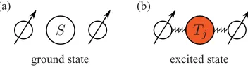
For our model we consider a structure comprising three integral components: two nuclear spin qubits, labeled n and n, and a mediator spin system with an optical degree of freedom. We denote the ground state of the mediator |0 and the first excited state |e. Further, |0 is assumed to be spin-silent, while |e possesses an electronic spin-1 character. The spin-1 (quasi)particle is thus created upon optical excitation of the mediator system. Importantly, the two spin qubits do not directly interact with each other, yet both are coupled to the excited state of the mediator with an isotropic Heisenberg interaction as depicted schematically in Fig.1. The Hamiltonian for such a three-particle system in an external magnetic field is then given by

H = −ωnSz,n−ωnSz,n+ |e(ωeSz,e+ω0)e|

+ |eASn· Se+ASn· Se+DSz,e2

e|, (1)

whereωn/ndenotes the Zeeman splitting of the two qubits and

ωe that of the central spin-1 particle;D is the uniaxial zero-field splitting,AandAare the isotropic Heisenberg coupling constants, and ω0 denotes the (typically optical) excitation

energy of the mediator. HereSz,n/n/eandSn/n/eare the usual component and total vector Pauli spin operators, respectively. Hamiltonian (1) can describe many different nanostruc-tures, in particular, a range of optically active molecules, in which case the mediator ground (excited) state corresponds to the absence (presence) of an electron-hole pair. The transition between these two states can be induced by a short laser pulse of frequency ω0; moreover, the excited state will

decay naturally through spontaneous emission. By contrast, a nitrogen-vacancy center in diamond surrounded by two13_C

atoms [25] is an example of a system in which the spin-1 mediator is not susceptible to decay and is ever present. Many of the results discussed in this article are equally valid for this kind of system. However, the following discussion primarily focuses on the example case of the molecular system consisting of a functionalized C60 molecule with two functional groups

as depicted in Fig.2.

In what follows we first analyze the Hamiltonian, Eq. (1), for two cases: that of a symmetric and that of an asymmetric system. In order to understand the system properties and dynamics, we determine the eigensystem using perturbation theory. This will provide us with the necessary basis to design suitable protocols for the controlled generation of nuclear spin entanglement for both these cases.

ground state excited state

(a) (b)

FIG. 1. (Color online) (a) There is no coupling between the mediator and the two nuclear spins in the ground (or vacuum) state

|0. (b) The excited state of the mediator (e.g., an electron-hole pair) has spin-1 character and couples to both nuclear spins.

FIG. 2. (Color online) A functionalized buckyball with two satellite atoms [far left and far right (blue) spheres]. In reality the functional groups are likely much larger than a single atom, but for simplicity we depict here only the two relevant atoms with a nuclear spin 1/2, for example,13_C,15_{N, or}31_{P. Note that the two satellites}

(or, rather, functional groups) are not necessarily both the same and that the system may thus be “asymmetric.”

III. EIGENSPECTRUM AND EFFECTIVE HAMILTONIAN A. Symmetric system

By definition, the symmetric system consists of two nuclear spins withωn=ωn and equal hyperfine coupling constants

A=A. In the presence of the electronic excitation, i.e., after the application of a suitable laser pulse, the Hamiltonian governing the spin dynamics is given by

Hsym= e|H|e = −ωnSz,n+ωeSz,e−ωnSz,n

+A(Sn· Se+Sn· Se)+DSz,e2 , (2)

where we have neglected the termω0, which is proportional

to the identity and unimportant for the dynamics. Since the electronic Zeeman splittingωeis typically the highest energy scale of the system (and, in particular, much higher thanωn), it is safe to assume that

|ωn|,|D|,Aωe. (3)

Based on the above assumption, we employ degenerate perturbation theory to determine the eigenspectrum ofHsym.

We begin by partitioning the Hamiltonian as

H_sym =H₀,sym+Hsym , (4)

where

H0,sym= −ωnSz,n+ωeSz,e−ωnSz,n+DSz,e2 (5) is treated exactly, and the perturbation is given by

H_sym =A(Sn· Se+Sn· Se). (6)

AsH₀,symis diagonal in the computational basis (defined as {|en₁n₂|e=T_±,T₀andn₁/2= ↑,↓}) and↓↑|H0,sym|↓↑ = ↑↓|H0,sym|↑↓, degenerate perturbation theory is required.

Making use of assumption (3) we then get the second-order eigenenergies,

Ej,1=Ej,3−εj, Ej,2 = −j ωe+ |j|D, (7) Ej,3=Ej,2−δj, Ej,4=Ej,2+εj, (8)

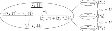
with the corresponding eigenvectors up to first order (see Fig.3),

|Ej,1 = |Tj ↓↓, |Ej,2 =

1 √

2(−|Tj ↓↑ + |Tj ↑↓), (9)

|Ej,4 = |Tj ↑↑, |Ej,3 =

1 √

2(|Tj ↓↑ + |Tj ↑↓), (10)

and where we have defined the following quantities for compactness:

ε₋=ωn−A+2a₋,ε0=ωn+2a+, and ε+=ωn+A; (11) δ₋= −2a₋, δ0= −2a0, and δ+=2a+; (12)

a_±=1 2

A2

∓D+ωe+ωn and a0=a+−a−. (13)

Based on this spectrum, we now approximateHsym in the

following way to obtain an effective Hamiltonian:

Hsym ≈V†diag(E−1,1, . . . ,E1,4)V =:Hsym, eff, (14)

where V is the matrix of the approximate eigenvectors (see Fig.3),

V =(|E₋,1|(E−,2 · · · |E+,4). (15)

In the computational basis,H_{sym, eff}consists of three blocks with the following structure:

⎛ ⎜ ⎝

× × × × ×

× ⎞ ⎟

⎠, (16)

where×denotes a nonzero entry and each block belongs to one of the three spin statesT₋,T0, orT+. Correspondingly, we define the three subspaces Tj spanned by the vectors |Tj ↓↓|Tj ↓↑, |Tj ↓↑, |Tj ↑↓, and |Tj ↑↑, with j = −,0,+. In this paper, the indexj denotes the electronic spin state of the excitation, whereas the letterialways indexes the four nuclear spin states.

In writing Eq. (14) we have neglected all matrix elements between subspace Ti and subspace Tj (i=j); the effect of these matrix elements is negligible because the electronic Zeeman splittingωeis much larger than the nuclear Zeeman splittings. The dynamics in each of theTj is therefore closed

FIG. 3. Eigenspectrum of a symmetric system up to second order of perturbation theory (eigenvectors not normalized). Our basis states obey the relations Sz,e|T± = ∓|T±, Sz,e|T0 =0, Sz,n| ↓ = | ↓, andSz,n| ↑ = −| ↑.

and can be described by an effective 4×4 Hamiltonian of the form given above. We now analyze the nuclear spin dynamics arising from each of those effective subspace Hamiltonians. A term in the Hamiltonian that is proportional to the identity has no effect on the dynamics within the subspace, so we can subtract D+ωe+a−, a0, and D−ωe−a+ from the subspace Hamiltonians for T₋, T0, and T+, respectively

(thereby neglecting unimportant phases that are common to all states in each block). We can simplify the resulting HamiltoniansHsym, eff,j further by transforming to a suitably chosen rotating frame through the transformation

H_{sym, eff, j} =UjHsym, eff,jUj†+iUj dU_j†

dt , (17)

where

Uj(t)=Rz,n(φjt)⊗Rz,n(φjt) (18) and

φ_±= −ωn∓A−a±, (19) φ0 = −ωn−a−−a+, (20)

Rz,i(φ)=exp(−iSz,iφ). (21) In this rotating frame we obtain the Hamiltonians

H_{sym, eff, j} =k(j)2aj(Sx,nSx,n+Sy,nSy,n), (22) where k(j)=1,1,−1 (with j = −,0,+, as it will be throughout the paper). Each of these effective subspace Hamiltonians therefore induces the dynamics of a direct XY coupling of the two nuclear spins, with a time evolution corresponding to Rabi flopping between nuclear spin state |↓↑ and nuclear spin state |↑↓. The Rabi frequency aj depends on the spin statejof the optical excitation. According to Eq. (13), we expecta₊to be fairly similar toa₋, whereas, in comparison,a₀will be much smaller.

We return to the symmetric case to discuss entanglement generation in Sec.IV Abut first complete our analysis of the Hamiltonian for nonsymmetric cases.

B. Asymmetric system

Next we consider an asymmetric system with unequal nuclear Zeeman splittings and/or unequal nuclear-electronic excitation hyperfine coupling. The excited state Hamiltonian is then given by

H_asym= e|H|e = −ωnSz,n+ωeSz,e−ωnSz,n+ASn· Se

+ASn· Se+DSz,e2 . (23)

For the purpose of applying perturbation theory, we consider the nuclear-spin-mediator coupling as the perturbation and split the Hamiltonian as follows:

H0,asym= −ωnSz,n+ωeSz,e−ωnSz,n+DSz,e2 , (24) H_asym =ASn· Se+ASn· Se. (25) For the asymmetric system we assume that the parametersA andAandωnandωndiffer sufficiently to fulfill the following two inequalities

1

2|A−A±(ωn−ωn)| |a±|,|a±|, (26) 1

where aj anda_j are as defined in the previous section, with the latter usingωnandArather thanωnandA. Under these assumptions, nondegenerate perturbation theory can be used for calculating the eigensystem. The state corrections to first-order perturbation theory then introduce a small mixing of computational basis states with corrections of magnitude

1 √ 2

A

D±(ωe+ωn) and 1 √ 2

A

D±(ωe+ωn), (28) which are negligible forA,Aωe. The eigenstates ofHasym

thus coincide with those of H0,asym (which are simply the

computational basis states) to a very good approximation. Analogously to our approach in the symmetric case, we proceed by analyzing individual effective Hamiltonians for the subspacesTj (j = −,0,+). After adding a suitable constant to each subspace, we obtain three diagonal Hamiltonians,

Hasym, eff,j =φjSz,n+φjSz,n, (29) whereφ_j andφj are as defined in Eqs. (19) and (20) and the prime denotes that ωn andA are used for the expression, instead of ωn and A. All three effective Hamiltonians are local, meaning that there is no direct coupling between the two nuclear spins.

C. Crossover between a symmetric and an asymmetric system In a certain region of parameter space neither the symmetric nor the asymmetric analyses are justified. In this section we consider this “crossover” regime, so that in the later discussion we will be able to interpolate between those two cases.

We start with the approximated symmetric Hamiltonian Hsym,effand treat the asymmetry as the perturbationHco , i.e.,

Hco=Hsym,eff+Hco , (30)

H_co = −1ωnSz,n+2ASn· Se, (31) where1is the fractional difference between the two nuclear

Zeeman splittings, 1= ωnω−nωn, and 2 is the fractional difference between the two coupling constants,₂= A_A−A.

We begin with the vectors |Ej,i and values Ej,i (j = −,0,+; i=1, . . . ,4) from Sec. III Aas the eigenstates and eigenvalues of HamiltonianHsym,eff. As in the other two cases,

we can still neglect those terms ofHcowhich couple different

projections of the excitation spin with strength2K/ √

2 since the relevant states differ in energy by about ωe, yielding an effective crossover HamiltonianHco,effwith the eigenvectors

|Ej, 1 = |Tj ↓↓,

(32)

|Ej,2 =

1 √

2(αj,2,1|Tj ↓↑ +αj,2,2|Tj ↑↓),

|Ej, 3 =

1 √

2(αj,3,1|Tj ↓↑ +αj,3,2|Tj ↑↓), (33)

|Ej,4 = |Tj ↑↑,

where

|αj,2,1/2|2= |αj,3,2/1|2=

1 2

⎛

⎝1±sgn(aj)fj a_j2+f_j2

⎞ ⎠ (34)

and

f_±=1₂(2A±1ωn) and f0= −1₂1ωn. (35)

The corresponding eigenvalues are

Ej,1/4=Ej,1/4±k(j)fj, (36)

Ej,2/3=Ej,2+k(j)

aj ∓sgn(aj)

a2

j +fj2

, (37) wherek(j) is again 1, 1,−1 forj = −, 0, +, respectively.

It is easy to see that the eigenstates reduce to those of the symmetric case for a vanishing perturbation (fj =0), whereas they tend to the computational basis states for a larger perturbation as required for the asymmetric system (|fj| |aj|).

IV. CONTROLLED GENERATION OF ENTANGLEMENT The contrasting analyses presented in the previous section suggest that the dynamics of the system will vary significantly depending on its parameters. Therefore, different approaches for achieving controlled entanglement between the two nuclear spins will be required. In this section we show how to do this in each case; we begin with the symmetric system introduced in Sec.III A.

A. Symmetric system: Entangling time evolution For the symmetric system, we exploit the effective XY coupling between spin state|↑↓and spin state|↓↑for the generation of entanglement. The fact that the magnitude of this coupling depends on the spin state of the excitation will allow us to control the interaction.

The free time evolution in any of the subspacesTj takes suitable initial product states of the nuclear spins to entangled states at certain subsequent points of time. In order to quantify the performance of the desired operation, we consider the entangling powerof the unitary operator that describes the time evolution of the system. The entangling power is defined as the mean linear entropy produced by the unitary operator acting on a uniform distribution of all (pure) product states [27]. A maximally entangling two-qubit gate, e.g., the controlled-NOT (CNOT) or the controlled-PHASE(CPHASE) gate, possesses an entangling power of 2/9.

For the symmetric system the entangling power of the free time evolutionUj(t)=exp(−iH_{sym,eff, j}t) is given by the fol-lowing simple expression for each of the three subspacesTj:

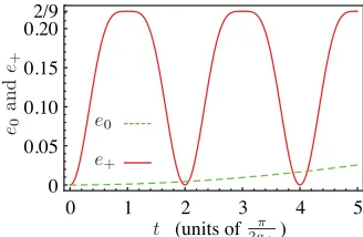
ej =1₉[3+cos(2ajt)] sin2(ajt). (38) The entangling power ej is only a function of the coupling strengthaj between state|Tj ↓↑and state|Tj ↑↓, becoming maximally entangling at times that are odd-integer multiples oft_max=π/(2aj). However, the characteristic time scale over which entanglement builds up differs significantly between the subspaces, sincea_±/a0=ωe/(2D) to leading order, and

this ratio is typically much higher than 1. Hence, e0(t)≈0

fort < π/(2a_±) when|D| ωeas we have assumed so far. Figure4shows the entangling powerse₊ande0 for a typical

FIG. 4. (Color online) Entangling powere+/0of the time

evolu-tion operatorsU₊/0(t). Herea+=32a0(see text).

Based on these observations, we can formulate a protocol for the controlled generation of entanglement. Consider a system that is initially in its ground state (i.e., there is no excitation coupling to the nuclear spins). A laser pulse creates the excitation, which will, in general, be in a mixture of the three spin states |T₋, |T0, and |T+. For the present discussion, we assume it to be in state|T0; the discussion

of a mixed initial state follows later. A short microwave pulse allows us to flip the state of the excitation selectively to either the |T+ or the |T− state since the transition frequencies are split by the zero-field splitting. The entangling dynamics proceeds much more rapidly in these outer subspaces, reaching the first entangling power maximum after a timet = π

2a±. We

can now apply another microwave pulse to flip the excitation back into the|T₀ state, where the further evolution is much slower and entanglement can be preserved.

There are, however, a few subtle points worth pointing out. First, similar to the case of applying the maximally entangling CNOT operation, only suitable initial states will evolve into entangled states. Second, certain particular input states can reach maximal entanglement in less time than π

2a_±; for example, the time evolution U(₄π_a

+) takes |T+↓↑ to a

maximally entangled state.

Finally, the (optical) excitation, whose natural lifetimeτ is assumed to be longer than the time it takes to build up the entanglement ₂π_a

± < τ, needs to be destroyed quickly enough

so that no further (slower) evolution unwinding the achieved entanglement occurs in theT0subspace. This can be achieved

either with a coherent optical π pulse or, alternatively, by simply waiting for the system to decay back to its ground state if the following hierarchy of time scales exists in the system,

π

2a_± < τ π 2|a0|

. (39)

However, in contrast to the de-excitation with a coherent laser pulse, it is not immediately obvious that the nuclear spin entanglement can survive the optical decay process; we therefore now take a small diversion to analyze this decay process in detail.

1. Decoherence due to the optical decay process

In general, the optical decay of the mediator induces decoherence on the nuclear spins. In order to quantify this,

we make use of the quantum optical master equation (for a full derivation see, e.g., Ref. [28]):

d

dtρ˜(t)=

ω,ω

ei(ω−ω)t(ω)[A(ω) ˜ρ(t)A(ω)†

−A(ω)†A(ω) ˜ρ(t)]+H.c., (40)

where ˜ρdenotes the density matrix in the interaction picture, (ω) is the rate for a transition with frequencyω, and H.c. is the Hermitian conjugate. The sum is taken over all optical transitions of the system with transition operators A(ω) as defined by

A(ω)= E−E=ω

(E)D(E), (41)

where E and E are eigenvalues of H that differ by ω and (E) denotes the projection onto the eigenspace belonging to eigenvalue E. D denotes the system’s op-tical dipole operator. The symmetric system features 12 optical transitions, |eTj ↓↓ → |0↓↓, |eTj√1

2(∓|↓↑ +

|↑↓)→ |0√1

2(∓|↓↑ + |↑↓), and|eTj ↓↓ → |0↓↓, for

j = −,0,+. We make the additional assumption that the optical decay rates are all equal and can thus be characterized by a single optical lifetimeτ.

Equation (40) can often be simplified by applying an instance of a rotating-wave approximation (RWA), based on the assumption that fast-oscillating terms average out [28], giving this more common form of the quantum optical master equation:

d dtρ˜(t)=

ω

(ω)[A(ω) ˜ρ(t)A(ω)†−A(ω)†A(ω) ˜ρ(t)]+H.c. (42) However, the RWA is only justified when |ω−ω|−1 is small compared to the relaxation time of the system τ. Under the assumptions of Eq. (39), this is fulfilled ex-cept for the two transition frequencies ω1=E0,2+ω0 and

ω₂=E₀,2+ω0−δ0, which correspond to the transitions

|eT0√1₂(∓|↓↑ + |↑↓)→ |0√1₂(∓|↓↑ + |↑↓). Therefore

we can safely apply the RWA to all remaining frequencies, obtaining

d dtρ˜(t)

=

ω,ω_∈S

ei(ω−ω)t(ω)[A(ω) ˜ρ(t)A(ω)†

−A(ω)†A(ω) ˜ρ(t)]

+

ω∈S

(ω)[A(ω) ˜ρ(t)A(ω)†−A(ω)†A(ω) ˜ρ(t)]+H.c.

(43)

=

ω

(ω)[A(ω) ˜ρ(t)A(ω)†−A(ω)†A(ω) ˜ρ(t)]

+e2a0it 1

2τ[2A(ω1) ˜ρ(t)A(ω2) †

whereS= {ω₁,ω₂}and, using phenomenological decay rates,

(ω)= ₁

2τ if ω >0,

0 if ω <0. (45)

This definition of decay rates describes the typical situation of only spontaneous emission occurring, since stimulated emission or absorption of photons is proportional to the negligible power density of thermally activated photons in the environmental modes.

Rather than solving the above master equation for the entire Hilbert space of our system, we are interested here only in the 4×4 density matrix ρf _{of the two nuclear spins after the} decay has occurred:

ρf := 0|ρ˜(t= ∞)|0. (46) Limiting the following discussion to this nuclear spin sub-space, it is easy to see that only a small number of elements ofρf _{can be populated by the decay process. These nonzero} elements are ρ_a,bf witha =b= ↓↓,a=b= ↑↑, anda,b∈ {↓↑,↑↓}. The final nuclear spin state after the optical decay can be compactly written as

ρ_a,bf = eT0a|ρ˜0|eT0b + 1₂

j=±

(eTja|ρ˜0|eTjb

+ eTja|ρ˜0|eTjb), (47)

where ˜ρ0=ρ˜(0) is the full system’s density matrix in the

interaction picture before the decay process and the bar on top of the nuclear spin states denotes that these are flipped, i.e.,

↓ = ↑ and↑ = ↓. Hence the coherences between |eT_±↓↑

and|eT_±↑↓do not necessarily survive, but all the coherences between|eT0↓↑and|eT0↑↓survive the optical decay,

re-flecting the fact that no RWA approximation has been made for the transitions |eT0(±|↓↑ + |↑↓)→ |0(±|↓↑ + |↑↓).

Physically, this means that these two transitions produce indistinguishable photons due to overlapping emission spectra. In the absence of other decoherence processes, the spectra are simply given by lifetime broadened Lorentzians [29]:

L(ω)= 1/τ

(ω−ωi)2+_(1/τ)2 for i=1,2. (48)

The photons emitted in all 10 other transitions can, in principle, be distinguished, so that we are effectively dealing with 11 distinct, incoherent decay channels. It is worth noting that there are three decay channels which populate the|0(±|↓↑ + |↑↓) states, one each for the excitation spin projectionsT0,_±, but only the decays from theT0subspace preserve coherence.

In Fig. 5 we plot the purity Tr[ρ(t)2_{]=Tr[ ˜ρ(t)}2_{] to}

illustrate the decoherence induced by the optical decay for three different initial density matricesρi(0)= |ψiψi|with

|ψ1 = |eT+ ↑↓, |ψ2 = |eT0↑↓, and

|ψ3 = 1₂|eT0(|↓↓ + |↓↑ + |↑↓ + |↑↑). (49)

Solving master equation (43) analytically, we then obtain the following final density matrices of the nuclear spins after the decay:

ρ₁f = 1

2(|↓↑↓↑| + |↑↓↑↓|), (50)

FIG. 5. (Color online) Evolution of the purity Tr[ρ(t)2_{] of a}

system initialized in an excited state during the optical decay process. The three different initial states shown are defined in (49), and τ δ0=0.05π.

ρ₂f = 1 2+2δ2

0τ2

δ₀2τ2|↓↑↓↑| +iδ0τ|↓↑↑↓|

−iδ₀τ|↑↓↓↑| +2+δ2₀τ2|↑↓↓↑|, (51)

ρ₃f = 1₄(1+ |↓↑↓↑| + |↑↓↓↑|), (52)

with the corresponding purities

Trρ₁f2 =1/2 and Trρ₃f2=3/8, (53) Trρ₂f2 = 2+δ

2 0τ2

2+2δ2 0τ2

(39)

≈1−δ

2 0τ2

2 . (54)

At first it may seem surprising that an initial state|eT₊|↑↓ can end up in a complete mixture of|0|↓↑and|0|↑↓. This is due to assumption (39), which underpins the optical master equation (43). This means that we have implicitly included the fast Rabi oscillations between |↓↑and|↑↓ in the T+ subspace while the system is waiting for the decay. In contrast, in theT0 subspace the inherent dynamics is much slower so

that the final result depends on the relative magnitudes ofδ0

andτ.

Perhaps surprisingly, decay due to the spontaneous emis-sion of a photon does not act as a source of decoherence if two conditions are met: (i) the system decays from the subspace spanned by the two states|T0↓↑and|T0↑↓; and

(ii)τ δ₀π, i.e., the energetic splitting of these two states is small compared to the inverse natural lifetime. This property can be turned into a powerful feature for suitable molecular systems, which we exploit in the following.

2. Dealing with a mixed electronic excitation

So far, we have assumed that the creation process yields a completely polarized excitation, enabling the simple protocol for the generation of entanglement described in a previous sec-tion. Motivated by recent experimental data from a promising candidate molecule [23], we now analyze the implications of having an initial mixture of the states |T0, and |T±.

lifetime of the excitation also depends on the state of the exci-tation, being much shorter for the|T₀state compared to|T±. In the following we demonstrate how the generic protocol presented earlier can be adapted to accommodate for the properties of the specific system presented in Ref. [23]. After a short laser pulse for the optical excitation, subspacesT0,±were found to be populated asp₋=0.49,p₀=0.02,and p₊= 0.49 with associated lifetimes τ₋=0.57 ms, τ0=0.02 ms,

and τ₊=0.57 ms. We assume that the nuclear spins are initialized in state|↓↑.

The basic idea of putting the system into |T_± states to let the free time evolution generate entanglement, followed by (mostly) switching off the interaction in theT0 subspace,

remains unchanged. As before, switching between different electronic states is accomplished using microwave pulses that are fast on the time scale of the nuclear spin evolution. The adapted protocol proceeds in two stages following the optical excitation. First, we let the desired entanglement build up in the T+ subspace by waiting for the time t= ₄π_a

+. We then

swap the populations of |T0 and |T+ and wait until the

entangled populations have decayed. The difference in decay rates 1/τ01/τ± means that the population of|T−largely survives once the majority of|T0has decayed to the ground

state. Second, population in the T₋ subspace is maximally entangled at times that are odd-integer multiples of π

4a₋. We pick the first such point of time after the|T0has emptied out

and apply another microwaveπpulse to swap the populations of|T0and|T−. Once more,|T0will quickly drain into the

ground state, meaning there is now no more excited population left. Ideally, we are left with an almost fully entangled nuclear spin state.

However, the success of the above-described protocol is predicated on the coupling strengthAof the nuclear spins to the excitation. In particular, for a very low coupling strength Ait takes a long time to entangle the nuclear spinst≈ π ωe

4A2, so

that there may be a substantial probability of the optical decay having occurred before the nuclear spins can become properly entangled. In this case the left-hand inequality of Eq. (39) is violated. On the other hand, if the coupling strengthAassumes very large values, then the right-hand side of inequality (39) is violated. In the latter case the photons resulting from the transitions|eT0√1₂(∓|↓↑ + |↑↓)→ |0√1₂(∓|↓↑ + |↑↓)

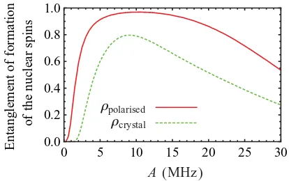
become distinguishable and the decay is hence no longer coherence preserving. In Fig. 6 we regard the hyperfine couplingAas a tunable parameter and plot the entanglement of formation (EF) [30] of the final state of the two nuclear spins. We consider two different initial states for the mediator spin: a completely polarized state and the mixed state reported in Ref. [23].

3. Robustness to imperfections in the symmetry of the system

The previously described protocol for the controlled gener-ation of entanglement assumes a perfectly symmetric system. In the following we analyze the degree of imperfection in the symmetry that may be tolerated. We already know that the crossover between the symmetric and the asymmetric case is not entirely abrupt. In Sect.III Cwe have found expressions for the eigenstates and eigenvalues that can fully interpolate between the symmetric and the asymmetric case. In this

0 5 10 15 20 25 30

0.0 0.2 0.4 0.6 0.8 1.0

Entanglement

of

formation

of

the

n

uclear

spins

A (MHz ) polarised

crystal

FIG. 6. (Color online) Entanglement of formation of the nuclear spins after applying our protocols as described in the text for different initial polarizations of the excitation:ρpolarized= |T0T0|(solid line)

and ρcrystal=0.49|T−T−| +0.02|T0T0| +0.49|T+T+| (dashed

line). For the first case we used the simple protocol described first in Sec.IV A2; the switching time used is π

4a₊. In the second case we use the enhanced protocol described at the end of the section; switching times here are π

4a₊ and 3π

4a₋. The nuclear spins for both curves are assumed to be initially in state| ↓↑; for parameters we use the values found in a recent characterization experiment [23]:D= −296 MHz, ωe=9.6 GHz, ωn=3.7 MHz, τ−=0.57 ms, τ0=0.02 ms, and

τ₊=0.57 ms.

crossover case, the effective Hamiltonian still consists of three distinct blocks, each corresponding to the spin state of the excitation|Tj(j = −,0,+), and matrix elements connecting the blocks are negligible due to the large energy difference ωe |ωn|. This allows us to assign a separate entangling powerej to the effective Hamiltonians describing each of the blocks.

We now give an easily provable lemma which will enable us to write the relevant analytic expressions of the entangling powersej for all three subspaces:

Lemma. LetHbe the time-independent Hamiltonian of two spin-1/2 particles with the following two properties.

(1) |E₁ = |↓↓, |E₂ = −a|↓↑ +b|↑↓, |E₃ =

b|↓↑ +a|↑↓, and |E4 = |↑↑, with |a|2+ |b|2=1, and

a,b∈Rare eigenvectors ofH.

(2) The eigenenergies ofHsatisfyE1−E2−E3+E4=0.

Then the entangling power of U(t)=exp(−iH t) is given by

e(b,β)=16 9 (b

2_−b4_{) sin}2

β 2

−32

9 (b

2_−b4₎2_sin4

β 2

,

(55) whereβ = |E₃−E₂|t. In addition, we havee(a,β)=e(b,β). Applying the above lemma to our effective Hamiltonians for the crossover case gives three expressionsej =e(cj,βj), with

βj =2t

a_j2+f_j2 and c2_j = 1 2

⎛

⎝1+ fj a2

j +fj2 ⎞ ⎠. (56)

It is easy to see that the parameteraj now directly competes with the strength of the perturbationfj in the expression for the entangling power. With the measure for the asymmetry

χj =

FIG. 7. (Color online) Entangling power ej of the free time evolution for an asymmetric system, when the excitation is in state

|Tjfor different strengths of the asymmetryχj. we can write the entangling power compactly as

ej =

3+4χ2

j +cos

2ajt

1+χ2

j

sinajt

1+χ2

j 2

91+χ2

j

2 .

(58) We plot ej for different asymmetries χj in Fig. 7. Not surprisingly, the entangling power decreases with increasing asymmetryχj. The maximum of the entangling power, which is achieved forβj =kπ, wherekis an odd integer, is given by

mj =16 9

c2_j−c4_j−32 9

c2_j−c4_j2=2 9

1+2χ2

j

1+χ2

j

2; (59)

this expression is plotted in Fig. 8. There is no significant reduction in the achievable entanglement power as long as χj <1/2, but the maximum drops quickly outside this regime. We note that for equal hyperfine couplings (₂=0) but unequal nuclear gyromagnetic ratios,

χ0

χ_± = a_±

|a₀| ≈

ωe

2|D| 1, (60) meaning that theT0subspace’s entangling powere0 is much

more affected by the asymmetry than e_±. Fortunately, the dynamics in this subspace is also the slowest, so that it can still conveniently serve as a shelf for entangled states generated in T₊ or T₋ until the optical excitation has been

2/9

0

0.20

0.15

0.10

0.05

0

1

2

3

4

5

FIG. 8. (Color online) Maximally attainable entangling powermj of the free time evolution, when the excitation is in state|Tjwith respect to the strength of the asymmetryχj.

de-excited or decayed. Importantly, Eq. (59) implies that our scheme is robust against the small deviations from a perfectly symmetrical system which one might expect in real-world experiments. Further, intentionally introduced small differences between frequencyωnand frequencyωn (e.g., a chemical shift caused by different surrounding environments) may actually be useful for individual control and tomography of the nuclear spins, while a high-fidelity entangling operation is still possible.

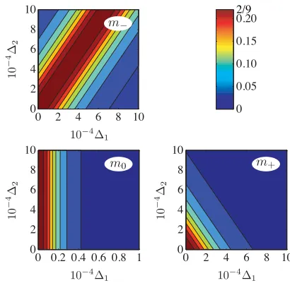
So far we have discussed the behavior of the entangling power in terms of the parameterχj. While the dependence of mjonχjis universal across the three subspacesTj, we obtain qualitatively different results when considering plots that are based directly on the1/2 asymmetry parameters. Figure9

shows the entangling power as a function of1 and2. We

see that the behavior is indeed quite different in each of the three subspaces: In theT₋subspace we obtain a ridge along which an asymmetry between the nuclear Zeeman splittings and the hyperfine coupling constants completely cancels out, meaning that a perfect operation is possible even for a system that is quite far removed from being symmetric. In contrast, the asymmetries add up in theT₊subspace, so that the error tolerance is much reduced in this case. Finally, theT0subspace

is only sensitive to 1, i.e., the difference in the nuclear

Zeeman splittings without any dependence on the hyperfine constants [see Eq. (35)].

The entangling power vanishes completely in the limit of an entirely asymmetric system [which we take to be defined by inequalities (26) and (27)]. In this case χj 1, and the eigenstates consequently coincide with the computational basis states, and the eigenvalues are such that the free time evolution no longer generates any entanglement (this result

FIG. 9. (Color online) Maximal attainable entangling powerm₋, m0,andm+as a function of the asymmetry in the Zeeman splitting 1=

ωn−ωn

ωn and hyperfine coupling asymmetry2= A−A

A . Other parameters areA=2.5 MHz,ωn=3.7 MHz,D= −296 MHz, and ωe=9.6 GHz. The entangling powermjonly reaches its maximum limit of 2/9 for certain values of1and2. See the text for a more

can be obtained by applying the above lemma). We analyze this situation in the following section.

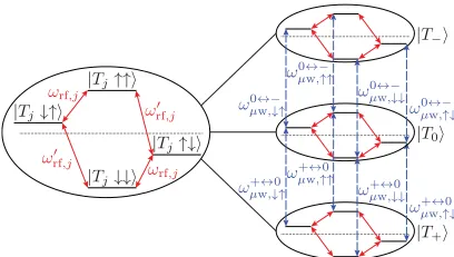
B. Control methods for the asymmetric system For an asymmetric system we cannot rely on the system’s free time evolution for the generation of entanglement; this is a direct consequence of the Hamiltonian being decomposable into local Hamiltonians [see Eq. (29)]. Therefore, we need to apply a suitable sequence of radio-frequency and microwave control pulses to accomplish our aim of creating an entangled nuclear spin state. Hence, we proceed by analyzing the dipole-allowed transitions of the asymmetric system (see Fig.10).

The asymmetric system possesses six (different) nuclear spin transitions on the radio-frequency scale, one per nuclear spin for each of the three spin states of the excitation. Referring to Sec.III Bwe obtain these from the second-order eigenenergies:

ωrf,j= |−j A−ωn−a₋(δj,₋+δj,0)−a+(δj,0+δj,+)|, (61) ω_rf,j= |−j A−ωn−a₋(δj,−+δj,0)−a₊(δj,0+δj,+)|, (62) whereδk,lis the Kroneckerδ, and as before,jindexes the spin state of the excitation|Tj. Further,ωrf,jdenotes the transition frequency of the first nuclear spin, and ω_rf,j the transition frequency of the second nuclear spin. In general, all six of these frequencies may be distinct.

Conversely, the spin state of the electronic excitation can be flipped conditional on the nuclear spin state using a suitable microwave pulse. With four nuclear spin states and two excitation spin transitions, this gives a total of eight microwave frequencies taking the excitation from|Tjto|Tj with (j,j)=(+,0) or (j,j)=(0,−), or vice versa. These are ω_μj↔_w,j_{↓↓/↑↑}=ωe+(−1)jD±1₂(A+A), (63) ω_μj↔_w,j_{↓↑/↑↓}=ωe+(−1)jD±1₂(A−A). (64) Here we have neglected second-order perturbation theory shifts proportional to aj anda_j, as these are typically very small compared toAandD.

Several possibilities exist for exploiting this rich transition spectrum in order to realize an entangling operation. In the following we discuss three methods in more detail: a single microwave 2πpulse, a pulse sequence of radio- and microwave pulses, and, finally, an adiabatic following method.

FIG. 10. (Color online) Microwave (dashed line) and radio-frequency transitions (solid line) of the asymmetric system. The computational basis states are eigenstates of the system Hamiltonian [assuming that Eqs. (26) and (27) are fulfilled].

1. CPHASEgate through a selective2πpulse

Simply applying a selective 2πpulse with the frequency of any of the microwave transitions given in Eqs. (63) and (64) naturally implements aCPHASEgate by imparting a phase of eiπ _{= −1 to only one of the four nuclear spin states [31].}

If the lifetime of the transition were infinite (and in the absence of other spin dephasing mechanisms), the 2π pulse could be made perfectly selective, achieved by a pulse that is long in the time domain and, accordingly, spectrally narrow in the frequency domain [32]. However, in practice, the optical lifetime will be finite and this may limit the selectivity and thus the amount of entanglement that can be achieved. The challenge is to find the right balance between a fast pulse that is only partially selective and a slow pulse during which the system suffers from the decoherence induced by the decay. We proceed by analyzing the trade-off that arises from these constraints in the following.

Suppose we are given an initial state that is an equal superposition of the computational basis states and a fully polarized state of the excitation,

|ψinitial = 1₂|T0(|↓↓ + |↓↑ + |↑↓ + |↑↑), (65)

and then apply a 2πmicrowave pulse with power0and with a

frequencyωDcorresponding to the energy difference between level|T₊↑↑and level|T₀↑↑. To describe the dynamics of the excited system we use either the effective asymmetric or the more general effective crossover Hamiltonian, whichever is more appropriate for the precise combination of system parameters in question. In particular, H_asym,eff,j is adequate whenever the eigenvectors closely coincide with the compu-tational basis states, whereasHco,eff,j is used otherwise. We apply the following criterion for discriminating between the two cases:

H_eff,j =

H_asym,eff,j|αj,2,1|20.001 or|αj,2,1|20.999,

Hco,eff,j 0.001<|αj,2,1|2<0.999,

(66) withαj,2,1 as defined in Eq. (34). In addition to the effective

system Hamiltonian Heff, we need to model the microwave

pulse (in the usual RWA), so that the total Hamiltonian during the pulse is given by

Hμw= |0(−ωnSz,n−ωnSz,n)0| + |eHeffe|

+|e(0Sx,e−ωDSz,e)e|. (67)

As this Hamiltonian is time independent, we can use a quantum optical master equation like the one defined in Eq. (43) to model the decay of the excitation in the interaction picture. The transition operators A(ω) are as defined by Eq. (41), with appropriate projectors onto the eigenspaces of Hμw. In

our calculations we perform the RWA in the master equation (remember that this RWA is different and independent from the RWA for the driving) whenever two frequencies differ by more than 30τ−1_{, whereτ denotes the lifetime of the excitation.}

driving invariably destroys the nuclear coherences. Therefore, we must use a different approach for taking the system back to its ground state. The first possibility is de-excitation using a resonant opticalπ pulse. Another option is to significantly “speed up” the decay process, e.g., by exciting the system into a different metastable excited state which is known to quickly decay to the ground state. Provided the lifetime of this metastable state is short enough, the wave function of the emitted photon does not carry information about the nuclear spin state, so that the nuclear spin coherence will be preserved. We assume that such a coherence-preserving de-excitation can be accomplished.

As mentioned above, the system is susceptible to potentially harmful decay events during the application of the 2π pulse, such that the final nuclear spin state ρnuc is a mixture of a

population that has spontaneously decayed and the remaining population to which the control sequence has been fully applied. Since we are now dealing with mixed statesρ_nuc, the entangling power is no longer a suitable measure for the quality of our operation, and as before we employ the entanglement of formation [30] as an alternative benchmark.

Assuming a simple top-hat pulse profile in the time domain, the pulse duration for a 2πpulse ist =√2π

20, where

₀is the applied microwave power. For optimal performance the right balance must be found between pulse selectivity and duration for each combination of system parameters and lifetimeτ. We thus maximize the achievable entanglement of formation by varying₀to obtain

E_F∗ =max 0

EF(ρnuc). (68)

As an example we chooseτ =10μs to plot the quantityE_F∗ in Fig.11as a function ofAandA. Larger hyperfine coupling constants allow a faster selective pulse, and the optimized entanglement of formation ofρnuchence increases withAand

A. Remarkably, even for a lifetime as short as 10μs, a high entanglement of formation can be obtained with only moderate hyperfine coupling strengths.

Finally, we note that the currently presented protocol also works for the symmetric system, where the entanglement operation then only takes a time t= ₂π_a

± ≈

π ωe

A2 , which is

much faster than our protocol discussed in Sec. IV A. For a short optical lifetime this approach may thus be advantageous, assuming that a spectrally narrow highly selective 2π pulse can be implemented.

2. Combined microwave and radio-frequency pulse sequence

In the previous section we discussed a simple imple-mentation of the CPHASEgate that is maximally entangling for suitable system parameters. However, other methods for creating maximally entangled states also exist, and these may be more advantageous if a particular final state is required. Here we briefly discuss an alternative control method that employs a sequence of microwave and radio-frequency pulses instead of a single microwave pulse. Let us assume that we have the initial spin state|T0↓↓and would like to create the

entangled Bell state √1

2(|T0↓↓ + |T0↑↑). It is impossible

to perform this operation with only radio-frequency pulses. However, we can achieve our aim by “shelving” parts of

(a)

(b)

1 5

10 15

20

1 5 10 15 20 0.7 0.8 0.9 1

EF after 2

pulse

Duration of 2

pulse (

s)

1 5 10 15 20 1

5 10

15 20 0

1 2 3 4

FIG. 11. (Color online) (a) Maximized entanglement of forma-tion of the nuclear spins after the 2π pulse with respect to the two hyperfine coupling strengths A and A. (b) Optimal duration t∗= _√2π

2∗₀ of the microwave 2π pulse with respect to the two hyperfine coupling strengthsAandA. We use the illustrative lifetime τ=10μs, while the other parameters used in this plot are motivated

by Ref. [24]:D= −320 MHz,ωe=9.7 GHz,ωn=5.97 MHz, and ωn=14.74 MHz.

the population in one of the other electronic spin states. An example of how this approach works in detail is depicted in Fig.12.

Of course, the microwave and radio-frequency pulses also need to be sufficiently selective for this approach, which imposes a minimal overall pulse sequence duration. Once more, we refrain from discussing sophisticated pulse shaping

FIG. 12. (Color online) Pulse sequence for the creation of the Bell state√1

2(|T0↓↓ + |T0↑↑). Black energy levels are populated

techniques [32], instead considering Rabi’s instructive formula for the transition probability of a driven two-level system,

P1→2(t)=

2

2+2 sin 2

(2₊2_{t), (69)}

where denotes the strength of the pulse, and the detuning. We apply this to the closest neighboring transitions of the (resonantly driven) target transition and demand that 2_/(2₊2_{)1 for all neighboring transitions, allowing a}

rough estimation of the duration required for each pulse in the sequence.

We take the example of a recent characterization experi-ment on an asymmetric system (phosphine oxide fullerene; DMFPH) [24], where the two nuclear spins of interest are provided by a hydrogen and a phosphorus atom in the functional group attached to the fullerene. The hyperfine coupling and the zero-field splitting were measured as

A≈6 MHz, A≈11 MHz, and D≈ −320 MHz (70) at an external magnetic field of B =0.346 T. Setting an upper bound of 0.01 for the unwanted transition probabilities, the four required pulses can all be applied in less than 1μs for typical nuclear gyromagnetic ratios. The duration of the pulse sequence is thus short compared to the expected optical lifetimes in candidate molecules, so that a high-fidelity entangling operation using this protocol should be feasible. However, we refrain from performing a more detailed analysis as in the previous section, since the results are similar and little additional insight is gained.

3. Implementation of aCPHASEoperation with adiabatic following

The last method discussed in this paper for creating entanglement in our system relies on the adiabatic following of system eigenstates, similar to the protocol described in Refs. [13] and [33]. Here, it is implemented by slowly modulating the intensity of a microwave pulse that is close to resonance with one or several of the microwave transitions of the excitation spin. Prior to the application of the pulse, the (asymmetric) system is prepared to be in a superposition of computational basis states as follows:

|ψinitial = |T0(a1|↓↓ +a2|↓↑ +a3|↑↓ +a4|↑↑), (71)

with normalization 4i=1|ai|2=1. Starting from this state,

the microwave power is then varied such that adiabatic following of instantaneous eigenstates occurs. Once the power is decreased again, all populations return to the computational basis. During the pulse, the eigenstates are energetically shifted and thus pick up a dynamic phase. However, the precise shifts of the states differ due to the the hyperfine coupling, so that, in general, each of the four states acquires a different dynamic phase. This gives rise to an overall combination that can be nontrivial and entangling [33].

Consider applying a microwave field with frequencyωD whose power envelope is changed gradually following a Gaussian function (t)=0exp[−(t /σ)2]. We apply this

Gaussian microwave pulse from an initial time t= −3σ to t=3σ and choose the frequency ωD in such a way that the pulse is off-resonant with all microwave transitions in

the system. The diagonal form of the system Hamiltonian H_asym,effpermits a description of the dynamics of each state in the superposition of Eq. (71) with a Hamiltonian connecting all three excitation states of the form

Hi(t)= i|H|i = ⎛ ⎜ ⎝

i,1 √(₂t) 0

_√(t)

2 0

_√(t) 2

0 √(t) 2 i,2

⎞ ⎟

⎠ (72)

written in the basis {|T₋i,|T0i,|T+i} for i={↓↓,↓↑, ↑↓,↑↑} with detunings i,1=ωμ0↔−w,i −ωD and i,2=

ω+↔_μw,i0−ωD. Note that the usual RWA has been performed. ChoosingωDsuch that, for eachi,

(t) √

2 2,i (73)

then enables us to write an approximate Hamiltonian for each of the nuclear spin states (valid to first order in perturbation theory) as

Hi,app(t)=

⎛ ⎜ ⎝

i,1 √(₂t) 0

_√(t)

2 0 0

0 0 i,2

⎞ ⎟

⎠. (74)

To achieve adiabatic following, the eigenenergies need to be varied slowly to suppress Landau Zener transitions between different eigenstates. Following Ref. [13], this can be accom-plished under the following conditions:

0

2_1,i σ for i= {↓↓,↓↑,↑↓,↑↑}. (75)

As we have mentioned above, the net effect achieved by the adiabatic pulse is the acquisition of a phase θi for each of the nuclear spin states. The “right” combination of control parametersσ,0, and1,i gives rise to an operation that is locally equivalent to aCPHASEgate if the following condition is met [13]:

π=θ1−θ2−θ3+θ4. (76)

In terms of the evolution of nuclear spins, the state|ψ_initialhas then evolved to

|T₀(a₁eiθ1|↓↓+_a

2eiθ2|↓↑+a3eiθ3|↑↓+a4eiθ4|↑↑), (77)

corresponding to a local phase on each nuclear spin in addition to the application of aCPHASEgate.

We now address the question of how the optimal combi-nation of control parameters may be found. The dynamical phase that is acquired by a state during the pulse is directly determined by the eigenenergy of the state|T0i, yielding

θi = − 3σ

−3σ 1 2

i,1−

2_i,1+2(t)2_{dt (78)}

= 0σ

2 3

−3

i,1

₀ 2

+2 exp(−2x2_{)dx. (79)}

Imposing condition (76) and solving forσ =σ(ωD,0) yields

σ = 2π ₀

3

−3

i

i,1

₀ 2

+2 exp(−2x2_)dx

−1

where the sum is taken over the four nuclear spin eigenstates. To mitigate the effect of decoherence caused by the decay of the excitation, we minimize the duration of the pulse under the constraint that the conditions in Eqs. (73), (75), and (76) are fulfilled, thus obtaining an optimalσ∗.

We incorporate the decoherence caused by the optical decay by modeling the time evolution with the Schr¨odinger picture master equation

d

dtρ(t)= −i[Happ(σ

∗_),ρ(t)]+ ω

(ω)[2A(ω)ρ(t)A(ω)†

− {A(ω)†A(ω),ρ˜(t)}] (81)

in Lindblad form [28].(ω) is as defined by Eq. (45) and the Lindblad operators A(ω) are determined by (41), where the projectors project onto the eigenspaces ofH_asym,effinstead of Happ. This simplification gives 12 (constant) incoherent decay

channels, rather than considering time-dependent Lindblad operators and re-evaluating the validity of the RWA at every instance in time (as would be required for the time-dependent Hamiltonian). Effectively, our approach then overestimates the destructiveness of the optical decay, thus giving a lower bound for the entanglement of formation of the nuclear spins.

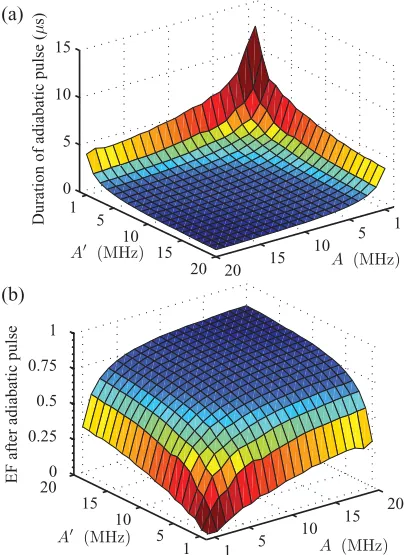
Figure 13 shows the results of a simulation that applies such an optimized Gaussian pulse with a pulse durationσ∗. For weak coupling strengthsAandA, this approach achieves a somewhat lower value of the entanglement of formation than the dynamic 2π pulse discussed earlier. However, a similarly high-fidelity entangling operation is possible for stronger

1 5

10 15

20

1 5 10 15 200 0.25 0.5 0.75 1

EF after adiabatic pulse

(a)

(b)

Duration of adiabatic pulse (

s)

1 5 10 15 20 1

5 10

15 20 0

5 10 15

FIG. 13. (Color online) (a) Optimal duration of the adiabatic pulse 6σ∗optimized overωDand0. (b) Entanglement of formation

after applying a Gaussian pulse whose duration is characterized by σ∗. As in Fig.11, other parameters areτ=10μs,D= −320 MHz, ωe=9.7 GHz,ωn=5.97 MHz, andωn=14.74 MHz.

hyperfine coupling. The term “adiabatic following” can invoke the impression that the desired operation will be much slower than a dynamical implementation. It is therefore astounding that our adiabatic pulse takes only about twice as along as the dynamic 2π pulse. Finally, we note that the adiabatic method (where the pulse is applied off-resonantly rather than having to hit a specific resonance) is inherently robust against pulse imperfections. This could be a significant advantage for experiments with ensembles of identical molecules. In this case, static and driving field inhomogeneities will inevitably lead to an over-or under-rotation of some of the ensemble spins when a dynamical pulse is applied (leaving the wrong excitation subspace populated), whereas the adiabatic approach ensures that all populations end up back in the correct spin levels.

V. SUMMARY

In this paper, we have given a detailed analysis showing how a transient optically excited state can be harnessed for the controlled generation of entanglement between two remote nuclear spins. We have identified control methods applicable over a wide range of system parameters and studied their performance with regard to the predominant decoherence mechanism. For a symmetric system consisting of two identical nuclear spins as qubits, the free time evolution is naturally entangling, but the characteristic time scale of the dynamics depends on the state of the excitation and can vary over several orders of magnitude, opening up the possibility of effectively switching the interaction on and off. For an asymmetric system, a different route needs to be taken, and we have presented one adiabatic and two dynamic methods for creating entanglement in this case. We have also included a discussion of the crossover regime between the asymmetric and the symmetric system to establish the robustness of the symmetric operation.

We have shown that the symmetric control method can be remarkably robust against uncertainty or fluctuations in the coupling constants and nuclear Zeeman splittings. As another advantage of the symmetric system, the system can decay back to the ground state without destroying the nuclear spin coherence. Conversely, for the asymmetric system additional control is required for the de-excitation step, yet it is easier to address the nuclear spins individually for single-qubit operations, initialization, and readout.

Interestingly, the active control methods proposed for the asymmetric system are much faster than waiting for the free time evolution in the symmetric case, and they can also be applied to the symmetric system if a short optical lifetime makes this approach advantageous. Finally, we note that the adiabatic control method is intrinsically more robust against control pulse and static field inhomogeneities, making it uniquely suitable for experiments with ensembles of identical systems. Astonishingly, the time required for such an adiabatic operation is only about twice as long as for its dynamical counterpart.

ACKNOWLEDGMENTS

by the Marie Curie Early Stage Training network QIPEST (Grant No. MESTCT-2005-020505), the EPSRC through QIP IRC (Grant Nos. GR/S82176/01 and GR/S15808/01), the

National Research Foundation and Ministry of Education, Singapore, the DAAD (German Academic Exchange Service), Linacre College, Oxford, and the Royal Society.

[1] Z.-Y. J. Ou and L. Mandel, Phys. Rev. Lett. 61, 50 (1988).

[2] E. Hagley, X. Maˆıtre, G. Nogues, C. Wunderlich, M. Brune, J. M. Raimond, and S. Haroche, Phys. Rev. Lett. 79, 1 (1997).

[3] M. A. Rowe, D. Kielpinski, V. Meyer, C. A. Sackett, W. M. Itano, C. Monroe, and D. J. Wineland,Nature409, 791 (2001).

[4] T. Wilk, S. C. Webster, A. Kuhn, and G. Rempe,Science317, 488 (2007).

[5] B. B. Blinov, D. L. Moehring, L.-M. Duan, and C. Monroe, Nature428, 153 (2004).

[6] M. Stobi´nska, G. J. Milburn, and L. Stobi´nski, e-print arXiv:0912.3547[quant-ph] (2009).

[7] S. C. Benjaminet al.,J. Phys. Condens. Matter18, S867 (2006). [8] T. D. Ladd, D. Maryenko, Y. Yamamoto, E. Abe, and K. M. Itoh,

Phys. Rev. B71, 014401 (2005).

[9] A. M. Stoneham, A. J. Fisher, and P. T. Greenland,J. Phys. Condens. Matter15, L447 (2003).

[10] S. C. Benjamin and S. Bose,Phys. Rev. Lett.90, 247901 (2003). [11] S. C. Benjamin, B. W. Lovett, and J. H. Reina,Phys. Rev. A70,

060305 (2004).

[12] S. Ashhab, A. O. Niskanen, K. Harrabi, Y. Nakamura, T. Picot, P. C. de Groot, C. J. P. M. Harmans, J. E. Mooij, and F. Nori, Phys. Rev. B77, 014510 (2008).

[13] E. M. Gauger, P. P. Rohde, A. M. Stoneham, and B. W. Lovett, New J. Phys.10, 073027 (2008).

[14] T. Yago, G. Link, G. Kothe, and T.-S. Lin,J. Chem. Phys.127, 114503 (2007).

[15] D. J. Sloop, H. Yu, T. Lin, and S. I. Weissman,J. Chem. Phys. 75, 3746 (1981).

[16] M. C. J. M. Donckers, A. M. Schwencke, E. J. J. Groenen, and J. Schmidt,J. Chem. Phys.97, 110 (1992).

[17] V. Zimmermann, M. Schwoerer, and H. C. Wolf,Chem. Phys. Lett.31, 401 (1975).

[18] G. J. B. van den Berg, D. J. van den Heuvel, O. G. Poluektov, I. Holleman, G. Meijer, and E. J. J. Groenen,J. Magn. Reson. 131, 39 (1998).

[19] J. J. Morton and B. W. Lovett,Annu. Rev. Condens. Matter Phys. 2, 189 (2011).

[20] T. Malyet al.,J. Chem. Phys.128, 052211 (2008). [21] A. B. Barneset al.,Appl. Magn. Reson.34, 237 (2008). [22] J. J. L. Morton, A. M. Tyryshkin, R. M. Brown, S. Shankar,

B. W. Lovett, A. Ardavan, T. Schenkel, E. E. Haller, J. W. Ager, and S. A. Lyon,Nature455, 1085 (2008).

[23] M. Schaffryet al.,Phys. Rev. Lett.104, 200501 (2010). [24] V. Filidouet al.(in preparation).

[25] P. Neumann, N. Mizuochi, F. Rempp, P. Hemmer, H. Watanabe, S. Yamasaki, V. Jacques, T. Gaebel, F. Jelezko, and J. Wrachtrup, Science320, 1326 (2008).

[26] L. Schiff,Quantum Mechanics Volume 1(McGraw-Hill, New York, 1949).

[27] P. Zanardi, C. Zalka, and L. Faoro,Phys. Rev. A62, 030301(R) (2000).

[28] H. P. Breuer and F. Petruccione,The Theory of Open Quantum Systems(Oxford University Press, New York, 2002).

[29] L. Mandel and E. Wolf,Optical Coherence and Quantum Optics (Cambridge University Press, Cambridge, 1995).

[30] W. K. Wootters,Phys. Rev. Lett.80, 2245 (1998).

[31] M. A. Nielsen and I. L. Chuang,Quantum Computation and Quantum Information(Cambridge University Press, Cambridge, 2000).

[32] M. A. Bernstein, K. F. King, and X. J. Zhou,Handbook of MRI Pulse Sequences(Elsevier, Amsterdam, 2004).