Bayesian methods for hierarchical distance sampling models

Bayesian methods for hierarchical distance sampling

models

C. S. Oedekoven

, S. T. Buckland

, M. L. Mackenzie

,

R. King

, K. O. Evans

, and L. W. Burger, Jr.

1

_{Centre for Research into Ecological and Environmental Modelling,}

School of Mathematics and Statistics,

University of St Andrews, St Andrews, KY16 9LZ, UK

2

_{Department of Wildlife, Fisheries & Aquaculture, Mississippi State University,}

Box 9690, Mississippi State, MS 39762, USA

*email:

[email protected]

Abstract

The few distance sampling studies that use Bayesian methods typically consider only line

tran-sect sampling with a half-normal detection function. We present a Bayesian approach to analyse

distance sampling data applicable to line and point transects, exact and interval distance data and

any detection function possibly including covariates affecting detection probabilities. We use an

integrated likelihood which combines the detection and count models. For the latter, counts are

related to covariates in a log-linear mixed effect Poisson model which accommodates correlated

counts. We use a Metropolis-Hastings algorithm for updating parameters and a reversible jump

algorithm to include model selection for both the detection function and count models. The

ap-proach is applied to a large-scale experimental design study of northern bobwhite coveys where

the interest was to assess the effect of establishing herbaceous buffers around agricultural fields

in several states in the US on bird densities. Results were compared with those from an existing

maximum likelihood approach that analyses the detection and count models in two stages. Both

methods revealed an increase of covey densities on buffered fields. Our approach gave estimates

model.

Keywords:designed experiments, hazard-rate detection function, heterogeneity in detection

prob-abilities, Metropolis-Hastings update, point transect sampling, RJMCMC.

1

Introduction

Bayesian methods are becoming increasingly popular for modelling wildlife populations and

abun-dances (e.g. Buckland et al., 2000, Marcot et al., 2001; Durban and Elston, 2005; Schmidt et al.,

2009; King et al., 2010). However, few distance sampling studies have taken a Bayesian approach.

Karunamuni and Quinn (1995) developed a Bayes estimator forf(0) using a half-normal

detec-tion funcdetec-tion (and a gamma prior), wheref(0)is a quantity estimated from the distance data that

allows observed counts to be adjusted for imperfect detection. The approach makes use of the

con-jugate property between the normal and gamma distributions. Other studies have built upon this

approach. Eguchi and Gerrodette (2009) extended this model by including a binomial likelihood

for the encounter rate along the line and described a joint posterior distribution for the density

model and effective strip width. Gimenez et al. (2009) implemented an estimator for f(0) using

BUGS software, while Zhang (2011) developed an empirical Bayes estimator for f(0). These

studies follow a similar approach in that they present their methods for line-transect data and use

the half-normal detection function. We describe a Bayesian approach to density estimation from

distance sampling data for both line and point transect data applicable to any detection function

that uses a hierarchical modeling approach.

Hierarchical distance sampling models have also been developed by e.g. Royle and Dorazio (2008,

ch.7.1). These authors employ a likelihood that combines the detection function and the binomial

model using the marginal probability of encounter (estimated from the detection function) and a

data augmentation approach for unobserved groups. The data augmentation approach was adopted

approach for double observer data.

In contrast, we use an integrated likelihood that combines the likelihood components of the

de-tection and count models. For the latter, we use a Poisson likelihood for the distance sampling

counts that incorporates a component corresponding to the detection function, thus allowing for

undetected animals on the surveyed strip (line transects) or circular plot (point transects). In

com-parison to Eguchi and Gerrodette (2009) who use a binomial likelihood to scale up from density

at the line to density in the study area, our Poisson model relates animal counts to covariates via a

log-link function. This approach does not rely on random placement of samplers in the study area

to the same extent as the design-based approach for the binomial model (Hedley and Buckland,

2004). Similar to Chelgren et al. (2011), we include a random effect for site in the Poisson model

to accommodate correlated counts due to e.g. repeat counts at the same site. The parameter space

is explored using a Metropolis-Hastings (MH) updating algorithm so that different prior

distribu-tions for the parameters are easily implemented, and a reversible jump Markov chain Monte Carlo

(RJMCMC) algorithm allows for model uncertainty to be incorporated. This may include different

key functions for the detection function model and different covariate combinations for both the

detection function and the count models.

These developments were motivated by a large-scale experimental study to assess the effects of

establishing conservation buffers along field margins on density of several species of conservation

interest such as the northern bobwhite (Colinus virginianus). Pairs of points were set up at the edge of fields in farmland in 13 states in the USA. These pairs of points consisted of one point on

a buffered treatment field and one on a nearby non-buffered control field and will be referred to

as sites in the following. Point transect surveys of coveys (fall-winter stable social units of 10-15

individual birds) were conducted at least once but up to three times per year in autumn from 2006

to 2008.

In the following we begin by developing the integrated likelihood (section 2), describe the Bayesian

approach (section 3) and analyse bobwhite covey data using our Bayesian approach (and a

with existing studies using distance sampling likelihoods (section 5).

2

An Integrated Likelihood for Distance Sampling Data

To obtain abundance estimates of a population of interest using distance sampling methods, lines

or points may be placed in the study area according to some design (see Buckland et al., 2001,

for details). Each line or point is surveyed at least once following the distance sampling

proto-col where the observer travels along the line (line transects) or remains at the point for a fixed

amount of time (point transects). Detections are recorded along with the perpendicular distance

from the line to the detection or radial distance from the point to the detection. These distances

may be recorded exactly or in predetermined distance intervals. Thus, surveys of this type produce

two types of data: firstly, the observed distancesye withe = 1,2,3, ..., n(nbeing the total

num-ber of detections) or observed distances ni in each ofi = 1,2,3, ..., I distance intervals (where

PI

i=1ni = n); secondly, the observed number of detections or countsnp at line or pointpalong with the effort data which at bare minimum consists of the size of the search area. In case

de-tections are made of single animals, the observed counts at the line (point) are equivalent to the

number of detections at the line (point). These two types of data, distances and counts, give rise to

the two components of the integrated likelihood described in this section. However, if detections

are made of groups of animals (rather than single individuals), a third type of data generated from

a distance sampling survey is cluster sizesewhich represents the number of individuals within the

eth detected group. For simplicity, we ignore cluster sizes for this study. Methods could, however,

be extended to accomodate group sizes larger than one. This may be done by considering counts

of individuals (rather than detections) in the count model described below or by including a model

for cluster sizes. The latter may be desirable e.g. if group size data are overdispersed (e.g. Ca˜nadas

and Hammond, 2006; Schmidt et al., 2012).

In contrast to many existing covariate models for distance sampling data (e.g. Hedley and

of the data simultaneously - similar to e.g. Royle et al. (2004) and Sillett et al. (2012). It consists

of the likelihood components for the detection function, which is denoted byLy(θ)for exact

dis-tance data (see eqn (5) below for interval data), and the Poisson likelihood for observed counts,

Ln(β|θ). We use θ and β to summarise the detection function and Poisson model parameters,

respectively. These are defined in more detail below. The integrated likelihood is the product of

the two components:

Ln,y(β,θ) =Ly(θ)Ln(β|θ) (1)

(modified from Buckland et al., 2004, ch. 2). We consider each individual likelihood component

inLn,y(β,θ)and begin withLy(θ).

2.1

Likelihood component for the detection function

Letf(y|θ)denote the probability density function of observed distances which is given as:

f(y|θ) = _wπ(y)g(y|θ)

R 0

π(y)g(y|θ)dy

, (2)

where y is the observed distance from the line (point) and w is the truncation distance (i.e. the furthest distance from the line (point) included in the analysis, Thomas et al., 2010).π(y)describes

the expected distribution of animals with respect to the line (π(y) = 1/w) or point (π(y) = 2y/w2_).

The detection function g(y|θ) may be modelled e.g. as half-normal (g(y|θ) = exp (−y2/2σ2),

withθ = {σ}) or hazard-rate (g(y|θ) = 1−exp (−(y/σ)−τ), withθ = {σ, τ}). The likelihood

component, which is conditional on the number of detectionsn, may be expressed as:

Ly(θ) = n

Y

e=1

f(ye|θ), (3)

whereyerefers to theeth detection (Buckland et al., 2004).

When detections are recorded in distance intervals, let fi denote the probability that a detected

fi(θ) = ci R

ci−1

f(yi|θ)dy

w

R 0

f(yi|θ)dy

, (4)

where the truncation distance, w corresponds to the outermost cutpoint. Then, the multinomial likelihoodLyGreplacesLy in eqn (1) and may be expressed as:

LyG(θ) =

     n! I Q i=1

ni!

     I Y i=1

fi(θ)ni, (5)

whereniis the number of detected animals in theith interval.

Note that in eqns (3) and (5), detections from all sites are pooled in one detection function. For

modelling heterogeneity using multiple covariate distance sampling (MCDS) methods, the scale

parameterσ of the half-normal or hazard-rate detection function is modelled as a function of

co-variates (σ(z) = δ0×exp(PQq=1zqδq), whereδq, q = 0,1,2, ..., Qreplaceσ inθ) (Marques and

Buckland, 2003) and thezqrepresent the values of theqth covariate.

2.2

Likelihood component for the count model

For the log-linear Poisson model,Ln(β|θ)we begin by considering a study design which consists

of multiple sites each containing one or more lines (points) that are surveyed at least once. If all

sites contain only one line (point) and surveys are not repeated, each count may be considered

in-dependent under conditions described by Buckland et al. (2001). However, if sites contain clusters

of lines (points) and/or sites were surveyed more than once, this assumption is violated. We deal

with this by grouping counts from the same site and fitting a random effect coefficient for each site

in the following count model (see below in this section).

are seen as are missed within (Buckland et al., 2001). Thus densityDjpr may be expressed as:

Djpr =λjpr/ν(θ). (6)

For line transects, ν(θ) = 2lpRw

0 g(y|θ)dy, where lp is the length of the line surveyed; for point

transectsν(θ) = 2πRw

0 yg(y|θ)dy. These definitions for ν are given for the case where all

detec-tions are pooled in a global detection function. When modelling heterogeneity, e.g. using MCDS

methods, the effective area may vary between lines (points) and the globalνbecomesνjpr.

However, when replacing Djpr with a covariate model (Djpr = exp

β0 +bj+PKk=1xkjprβk

)

and rearranging eqn (6) we obtain a model for the expected countsλjpr which is now a function of

the density model parametersβand conditional on detection function parametersθ:

λjpr(β|θ) = exp β0+bj+ K

X

k=1

xkjprβk+ ln (ν(θ))

!

. (7)

Hereβ0 is the intercept,bj the random effect for sitej(bj ∼N(0, σ2b)), xkthek covariates,xkjpr the covariate values measured during visitrto that line or point andβkthe associated coefficients. Vectorβ ={β0, β1, β2, ..., βK, σb}denotes the parameters associated with the covariates affecting

densities and the random effect standard deviation. Eqn (7) is given for the general case where

lines or points that may produce correlated counts, due to closeness in space and/or due to repeated

measurements at the same line (point), are grouped together as sitej. The inclusion of a random effect for site accommodates covariances for these measurements. However, in cases where lines

(points) follow a random survey design (Buckland et al., 2001) and each line (point) is surveyed

only once, the random effect term may be omitted.

Using this model for λjpr, the likelihood for the count model (eqn 7), conditional on detection

function parametersθ, may be expressed as:

Ln(β|θ) = J Y j=1 Z ∞ −∞   Pj Y p=1 Rj Y r=1

(λjpr) njpr

exp (−λjpr) njpr!

×q 1

2πσ2

b

exp − 1

2σ2

b b2_j

!

whereJrefers to the total number of sites, andPj andRj refer to the total number of lines (points)

at and visits to the jth site, respectively. Ln(β|θ)forms the second likelihood component in eqn

(1). Note that in a maximum likelihood context the likelihood function including a random effect

(for which normality is assumed) is generally formulated with an integral as shown in eqn (8) as the

random effect is integrated out analytically (or by approximation) and the individual coefficients

bj are not estimated (e.g. McCulloch and Searle, 2001). In the Bayesian context, the random effect

is not integrated out analytically. Here, we use a data augmentation scheme where the individual

coefficients bj are included as parameters (or auxiliary variables) within the model and updated

within the MCMC algorithm (see below).

3

The Bayesian Approach

3.1

Hierarchical Models

Using a Bayesian approach, random effects models can be implemented using hierarchical

mod-els where the standard deviation of the random effect (σb from eqn (8)) is considered a random

variable with a distribution rather than as a fixed value (Davison 2003). Individual random effects

coefficients (bj from eqns (7) and (8)) are fitted in the model and updated at each iteration of the

chain in a Markov chain Monte Carlo (MCMC) algorithm.

Prior beliefs regarding the parameters, such as knowledge obtained from a previous study, may be

included in the current study via the prior distribution. This may allow inference on model

param-eters in cases where too few data exist in the current study to obtain maximum likelihood estimates

with great precision (e.g. Eguchi and Gerrodette, 2009).

3.2

MCMC Algorithm

An MCMC algorithm is used to explore the posterior distribution of the parameters given the data.

We focus on the MH update (Hastings, 1970; Metropolis et al., 1953) as some of the likelihood

functions that may be used to form the posterior conditional distributions of parameters are

non-standard (e.g. half-normal or hazard-rate detection function that may include a covariate model

for the scale parameter). In particular, we use a random walk single-update MH algorithm with

normal proposal density. The proposal variance for each parameter may be obtained via

pilot-tuning (Gelman et al., 1996). See Appendix 6.1 for details on the MH algorithm.

3.3

Model Selection: Reversible Jump MCMC

To discriminate between competing models, we treat the model itself as a parameter and form the

joint posterior distribution over both parameters and models. To explore this posterior distribution

we implement an RJMCMC algorithm (Green, 1995) where each iteration involves two steps; step

1: update parameters given the current model using the MH algorithm (within model move) as

described above in section 3.2; step 2: update the model using an RJ algorithm (between model

move). Posterior model probabilities are estimated as the proportion of time the chain spent in a

particular model after the burn-in.

For the RJ step, two main strategies may be followed. In cases where models differ only in the

combination of the same set of covariates, a single RJ step may involve going through each

covari-ate and proposing to delete or add it depending on whether it is in the current model or not. This

involves generating a value for the new parameter from a proposal distribution (if we propose to

add it) or setting it to zero (if we propose to delete it) and calculating the acceptance probability

each time we propose to add or delete a parameter.

In those cases where all parameters of the newly proposed model change, one RJ step involves

generating new values for all parameters of the new model and accepting or rejecting the new

model based on the above acceptance probability. A proposed move from a half-normal detection

function model to a hazard-rate model represents a simple example for this scenario. For further

4

Case Study

4.1

The Data

As part of a study to assess the potential benefits of herbaceous buffers around agricultural fields,

Mississippi State University, Department of Wildlife, Fisheries, and Aquaculture set up a

monitor-ing program usmonitor-ing point transects in a number of Midwestern and Southeastern states in the US

(Evans et al., 2013). Survey points located at the edge of the field were paired up: one point on a

buffered treatment field and the other on a non-buffered control field of the same agricultural use

and within 1-3km of the treatment point. Each pair of points will be referred to as a site in the

following. Repeat visits were made to each point during fall of three survey years (2006-2008),

and each detected northern bobwhite covey was recorded along with their estimated radial distance

to the point. To facilitate unbiased distance estimation, observers used satellite images of the point

location and surroundings to mark each detected covey. As no estimates of covey cluster sizes

were obtained, we model cluster densities (rather than densities of individuals).

Only those 11 among the 13 original states in our study were included in the analysis that

con-tained more than 50 detections of coveys: Georgia, Iowa, Illinois, Indiana, Kentucky, Missouri,

Mississippi, North Carolina, South Carolina, Tennessee and Texas. Within these states, 447 sites

were visited 1–3 times in each survey year. The number of sites per state ranged from 30 to 61.

Af-ter defining a truncation distance of 500m following recommendations of Buckland et al. (2001),

the analysed data included a total of 2545 detections with associated distances that were observed

during 2534 counts (number of counts by state: GA 190, IA 221, IL 162, IN 217, KY 218, MO

352, MS 236, NC 244, SC 250, TN 219, TX 225).

4.2

The Bayesian Approach

We used eqns (3) and (8) to form the integrated likelihood function as shown in (1). Potential

covariate Julian day which was centred around its mean before the analyses (for the Ln(β|θ) model only as it did not reveal any influence on detection probabilities during preliminary analyses

using Distance software, Thomas et al., 2010). See Evans et al. (2013) for ecological details on

modelling data from this study. Hence, eight different covariate combinations were possible for

the detection function while 16 were possible for the density model.

We assume that counts from the different points of the same sites were (positively) correlated in the

same manner as repeat counts of the same point. Hence, we included one random effect coefficient

per site in the model (as described in section 2.2) where the same coefficient applied to all repeat

counts at either of the two points belonging to the same site.

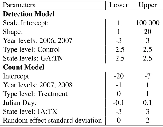
Uniform priors were placed on all parametersθ andβfor which bounds were chosen in

prelimi-nary analyses (Table 1). Generally this involved adding/subtracting two times the standard errors

from the maximum likelihood estimate of the full model; however, bounds were extended if a

pa-rameter value reached either of these. If the papa-rameter had natural bounds, e.g. zero for the lower

bound of the random effect standard deviation, these were adopted.

To make summary statistics of parameters directly comparable to the maximum likelihood

ap-proach (see section 4.3), the last covariate levels (in numerical or alphabetic order) of detection

function parameters were absorbed in the intercept to follow the parameterisation of factor levels

in Distance software. Likewise, the first levels were absorbed in the intercept for the count model

to follow parameterisation of factor levels in theglmerfunction from thelme4package in R. Preliminary investigation of the distance data indicated that the hazard-rate detection function

pro-vided a much better fit than the half-normal. Hence, we included eight different hazard-rate models

as choices for the probability density function of observed distancesf(y|θ)inLy(θ): one global

(with no covariates) and seven multiple covariate models. For the global model, only the scale and

the shape parameters required estimation (see section 2 for details). The multiple covariate models

contained additional parameters as the scale parameter was modelled as a function of one, two or

three of the covariates. For Ln(β|θ), λjpr from eqn (7) was modelled including a intercept and

investigated whether the count data were overdispersed. We fitted aglmmwith a quasipoisson dis-tribution using the full models for both detection and counts to calculate the offset. A quasipoisson

glmmcan be fitted using thegammfunction of themgcvpackage. The estimate of the dispersion parameter was 1.10. Hence, we assumed that Poisson was appropriate to use.

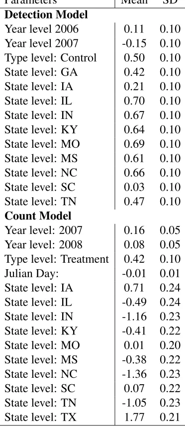
The chain was started without any covariates for the detection and count models. During a single

RJ step of each iteration, each of the covariates was proposed to be added or deleted depending on

whether it was in the current model or not. Valuesufor the new parameters contained in the new model were drawn from parameter-specific proposal distributions shown in Table 2. These were

initially defined as normal distributions with mean and standard deviation equal to the maximum

likelihood estimates and standard errors from the full models, however, we adjusted means (by

averaging estimates across different models for the respective parameters) and standard deviations

during pilot-tuning to improve model mixing.

To move from e.g. a global hazard-rate model to a model including a covariate, the global scale

parameterσwas converted intoδ0×exp(z1δ1)withσ=δ0 andu=δ1, whereδ1 is the coefficient

associated with covariatez1. The bijective function in this case (as well as in all the other possible

model moves) was the identity function similar to the example shown in Appendix 6.2. Therefore,

the Jacobian|J|(from eqn (12) in Appendix 6.2) equalled one. We assume that all models were

equally likely a priori, hence the probability of moving to modelmconditional on the chain being

in model m0, P(m|m0)was equal to P(m0|m) and vice versa for all possible model moves and

cancelled when calculating the acceptance probability (see eqn (12)).

Proposal distributions for the MH step were normal where the mean was the current value of

the parameter and the standard deviation was parameter-specific. The RJ and MH step together

completed one iteration. A total of 100 000 iterations were carried out where the first 10 000

were considered the burn-in period and ignored when obtaining model probabilities and summary

statistics for parameters. Visual inspection of raw trace plots from different starting points for

pa-rameters suggested that convergence had been achieved within 10 000 iterations.

priors for all parameters. We also tested the robustness of our estimated model probabilities by

starting the RJMCMC algorithm from the full detection and count models (as opposed to the

in-tercept only models). Both analyses revealed nearly identical results as those presented in section

4.4. Hence, we were confident that our results had converged.

4.3

The Classical Approach

To compare the Bayesian approach with the classical, the data were analysed using the two-stage

approach (Buckland et al., 2009), extended to include a random effect for site in the count model

(Oedekoven et al., 2013). The first step included fitting a detection function to observed distances

by maximising the likelihood in eqn (3). The same eight hazard-rate models were explored as in

the Bayesian approach, i.e. global and MCDS models with combinations of the covariates state,

typeandyear. The effective areaνjpr was estimated using the best model forf(y|θ).

In a second step, the effective area was incorporated into the count model forλjpr and parameter

estimates obtained using theglmer function of thelme4package (Bates, 2009b) in R. The likeli-hood for theglmerfunction is equivalent to eqn (8), except that the random effect is integrated out using an approximation for the integral (Bates, 2009a). The same 16 models were explored as in

the Bayesian approach including a fixed intercept and a random effect for site and combinations of

the four covariatesstate,type,yearandJulian day.

Best fitting models for both steps were found by minimum AIC values. As the effective area

rep-resents an estimate but is included in the model as if it was a known constant, non-parametric

bootstrapping was used to estimate uncertainty (bootstrap standard errors (BSE) and 95%

confi-dence intervals) of parameter estimates. To implement a non-parametric bootstrap routine with

999 repeats, an automatic model selection was set up in R that included calls to the MCDS engine

from the Distance software (Thomas et al., 2010) for the first step. For each bootstrap iteration,

sites were resampled with replacement until the original number of sites was obtained (Buckland

et al., 2009). To include model uncertainty in inference, the strategy followed was to select best

4.4

Results

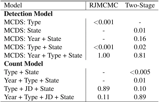
In the following we refer to those models with highest probabilities as the preferred models. For

the Bayesian approach, the preferred detection function model included the covariatesyear, type

andstatein the model for the scale parameter of the hazard-rate key function (probability = 1.00 to two decimal places, Table 3). Two other models were visited within the RJMCMC algorithm

with probabilities of<0.001 that included two (typeand state) or one covariate only (type). The same model with all three covariates was the preferred model for the two-stage approach having

been selected by AIC in 81% of bootstrap resamples. Three other models were selected: one with

covariatesyearandstate(16%), one withtypeandstate(2%) and one withstatealone (1%). For the count model, two models dominated the RJMCMC algorithm, the model with covariates

type, Julian day and state as the preferred model (0.89 probability) and the full model (year +

type+Julian day+state, 0.11probability, Table 3). For the bootstrap the latter was the preferred model, selected in 89% of resamples, while the former was the second most frequently chosen

model (10%). Two other models were chosen during the bootstrap including the covariates year,

typeandstate(1%) and the model including covariates typeandstate(<1%). Hence, the largest discrepancy in model probabilities between the two analysis methods was with regard to covariate

yearfor which the total probabilities to be included in any model was 0.11 for the RJMCMC algo-rithm and 0.90 for the bootstrap (Table 3). However, 95% confidence intervals obtained from the

bootstrap overlapped zero for bothyearcoefficients (Table 4) indicating that this covariate might have less importance than suggested by model probabilities for the bootstrap.

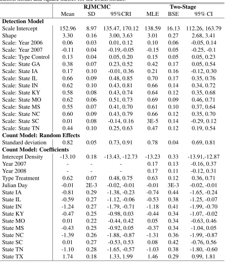
For the parameters of the detection function model, the posterior means of the parameters in the

preferred model were in most cases similar to the maximum likelihood estimates resulting from

the two-stage analysis of the original data (Table 4). The intercept for the scale parameter and the

shape parameter were larger for the Bayesian approach while the coefficients for the scale

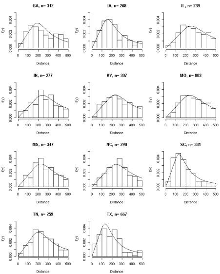
parame-ter were on average smaller. Histograms of detections by state and estimated expected probability

density functions (pdf) of observed distances from the Bayesian approach are shown in Figure 1.

coef-ficients for these states (Table 4). For these states, the steep decline after peak values for the pdf

indicated rapidly declining detection probabilities beyond∼100m (Figure 1).

Interestingly, measures of uncertainty were mostly smaller for the Bayesian approach despite the

fact that both stages from the two-stage approach were combined in one. The posterior standard

deviations were smaller than the bootstrap standard errors for all detection function parameters.

95% credible intervals were narrower than the 95% confidence intervals for all but four detection

function parameters (state coefficients IN, MS, NC and TN). Intervals from the two approaches

overlapped in all cases for the detection function parameters.

For the count model, means and intervals were again similar between the two approaches (Table

4). However, slight discrepancies in means for count model coefficients existed which might have

been due to that the best model from the two-stage approach contained the additional covariate

year and/or to Monte Carlo error. Further reasons are discussed in section 5. Also, measures of uncertainty were again mostly smaller for the Bayesian approach: standard deviations from the

Bayesian approach were smaller for all covariates in the count model compared to BSEs. 95%

credible intervals were narrower for all coefficients of the count model compared to 95%

con-fidence intervals, except for the covariate Julian day where they were equal. 95% credible and confidence intervals overlapped for all count model parameters. The only covariate selected for

the preferred count model for the two-stage approach that was not also in the preferred model for

the Bayesian approach wasyear. 95% confidence intervals for bothyearcoefficients included zero indicating that this covariate might have been negligible for the count model.

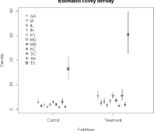
The parameter of interest in these models was the coefficient for the level Treatment of the type

covariate in the count model. This was 0.62 (SD=0.07) and 0.63 (BSE=0.12) for the Bayesian and

the two-stage approach, respectively, indicating an increase in covey densities on treatment plots

by 85% (E[exp(type coefficient)] =1.85) or 88% (exp(0.63)=1.88) by the respective methods. As described above, expected densities can be calculated using the values of theβparameters from

the count model. These values are obtained from the posterior distribution of these parameters for

eqns (6) and (7) for details). For calculating baseline estimates of the expected covey densities

for the RJMCMC algorithm and two-stage approach, we used those iterations from the

respec-tive methods where the preferred count model was chosen, excluding the burn-in iterations for the

RJMCMC. Using eqn (7), we set the covariates to those levels that were absorbed by the intercept

of the density model, i.e.year = 2006, type= Control, Julian day= 0 (which is equivalent to its mean as we centered the data for this covariate) andstate= GA and added a random effect contri-bution (0.5×σb2replacesbj from eqn (7) when calculating the average expected density across all

sites). The estimated baseline expected density from the RJMCMC algorithm was 2.91 coveys per

km2 (SD = 0.55, 95% CRI = (2.05, 4.14)). The posterior distribution of the expected density was

right-skewed with a mode of 2.60 coveys per km2. The estimated expected density resulting from

the two-stage approach was 2.44 coveys per km2 _{(BSE = 0.88, 95% CI = (1.25, 4.66)). Estimated}

expected densities for eachstateandtypecombination are shown in Figure 2.

5

Discussion

There are two main aspects in this paper that are innovative and deserve comparison to existing

methods. We present a novel approach for combining the likelihood functions for analysing

dis-tance sampling data in section 2 which is easily applicable to both interval and exact disdis-tance data.

We also present a Bayesian approach for analysing distance sampling data of multiple types in

a straightforward manner. Different detection functions (the half-normal, hazard-rate or others)

may easily be implemented. It may also be extended to include adjustment terms (added to the

half-normal or hazard-rate model, Buckland et al. (2001)) or covariates in the shape parameter. We

provide the R code as online supplementary material which is annotated for easy adaptation.

Bayesian methods have been used before for analysing line transect data with a global half-normal

detection function (e.g. Royle and Dorazio, 2008, ch. 7.1; Eguchi and Gerrodette, 2009; Gimenez

et al., 2009; Zhang, 2011), a half-normal with covariates (e.g. Gerrodette and Eguchi, 2011; Moore

simultaneous exploration of model and parameter space including different detection functions and

different covariate combinations for both the detection and count models via an RJMCMC

algo-rithm. Conn et al. (2012) described an RJMCMC algorithm for distance sampling data. However,

in their case, the RJ step refers to adding/deleting unobserved animals as part of the data

augmen-tation and not to exploring different models for the detection function or counts.

The log-linear Poisson model for counts described in section 2 does not depend on a random

sur-vey design in contrast with the classical distance sampling approach and data arising from sursur-veys

conducted from platforms of opportunity may be used (Hedley and Buckland, 2004). It allows

identification of relationships between abundance or density and parameters of interest, such as the

typecovariate in our case study, which may be of interest for designed experiments and wildlife management studies (see also Gerrodette and Eguchi, 2011). Similar to Hedley and Buckland

(2004) and Buckland et al. (2009), our count model may be extended to include smooth functions

for continuous covariates, e.g. by fitting polynomial splines using the B-spline basis, or the Poisson

likelihood may be replaced with a negative binomial likelihood if more appropriate, e.g. in case

overdispersion in the count data is present (e.g. Royle et al., 2004, Sillett et al., 2012).

Our approach is similary to Hedley and Buckland (2004) in that we use the conditional formulation

of the probability density function of observed distances (Buckland et al., 2001) and information

on detection probabilities enters the count model via an offset; we model counts asdensity× ef-fective area. However, Hedley and Buckland (2004) or Buckland et al. (2009) analyse their data in two stages. In their second stage count model, they condition on the estimate of the effective

area derived from the first stage detection model. This requires conducting non-parametric

boot-strapping so that uncertainty associated with estimating the detection function (and the effective

area) propagates into the second stage count model. Our integrated likelihood approach estimates

all parameters simultaneously allowing direct quantification of the precision of the parameters in

the count model with taking proper account of the estimation of detection function parameters.

Using the Poisson model with a random effect for estimating densities as defined in eqn (7) also

e.g. when there are repeat counts at the same line (point). This differs from the integrated

likeli-hood described by Royle et al. (2004). These authors considered the true but unknown abundances

at the site as a random effect with a Poisson distribution (in their notationNi ∼P oisson(λi)) and

integrate it out by summation. They derive a Poisson likelihood for the observed counts with

ex-pected value equal toλiπk(θ), whereπk(θ)is obtained using the unconditional probability density

function of observed distances and describes the probability that an animal occurs and is detected

in the kth distance interval. Hence, these authors model counts asabundance N × detected pro-portion of N for each interval. Note that we use the term integrated likelihood in the spirit of integrating the likelihood components pertaining to two different data types (described in section

2), while Royle et al. (2004) use the same term in the context of integrating out a nuisance

param-eter (although they combine the likelihood components from two different data sources as well).

In contrast to Royle et al. (2004), we model variations in observed counts between the different sites

(those variations not explained by any of the fixed effects included in the model) as a normally

dis-tributed random effect with mean zero, hence accounting for correlations between measurements

at the same sites. This represents an extension to Royle et al. who include one count per site in the

analysis. With the inclusion of site random effects, our approach allows us to incorporate repeat

counts from the same sites in the analysis. Our approach assumes that all counts from the same

site are positively correlated and only requires estimation of one additional parameter, the random

effect standard deviation. Chelgren et al. (2011) on the other hand, extended the approach of Royle

et al. (2004) by including a random effect for plot by week in the abundance model which requires

estimation of week-specific variance parameters. However, including random effects allows

infer-ence on the wider area that these sites represent and to obtain unbiased estimates of coefficients

retained in the count model. Bias in coefficient estimates may occur for example if some sites with

high bird densities were visited more frequently than those with low densities and this variation

was not modelled as a fixed or random effect.

The comparison of summary statistics for model parameters from the Bayesian approach with

4) which cannot be due to prior sensitivity as we used uniform priors on all parameters for the

Bayesian approach. We assume these differences may have been due to the fact that – as opposed

to the two-stage approach – the likelihoods for both components of our model were combined

for the integrated likelihood and influence each other. We argue, in concurrence with Johnson

et al. (2010), that simultaneous estimation of all parameters in one stage represents a more

realis-tic model without having to rely on the assumption of a true detection function model. Whether

the smaller uncertainty estimates from the Bayesian approach compared to the two-stage approach

were specific to our case study or can be expected in general is beyond the scope of this paper.

Our Bayesian approach provides improvements over previous approaches. Besides the often stated

benefits for Bayesian analyses, e.g. allowing for prior information to be included, our Bayesian

approach provided a particular benefit for using the integrated likelihood defined in section 2: it

might be challenging in some cases, such as our case study, to find the maximum likelihood

esti-mates for all parameters in one step. The covey data included a total of 2545 observed distances

during 2534 counts and the full model included 31 parameters with a random effect (447 sites).

Using maximum likelihood methods, the random effect coefficients are not estimated individually

but are integrated out during the optimisation of the likelihood. However, due to the integrated

nature of the detection and density models, functions such as glmerfrom the lme4package in R may not be used as these treat the offset as a constant. Using the hierarchical model set up for

the Bayesian approach, the random effect coefficients are included in the model specification and

updated during each iteration. Due to this data augmentation method, no numerical integration is

necessary providing a straightforward technique to explore the parameter space.

Bayesian methods also offer efficient exploration of model space with the use of RJMCMC. By

contrast, using a maximum likelihood approach, a model selection routine that considered all

pos-sible model combinations for our case study would have required maximisingLy,n(β,θ)for 128

models (possible combinations of eight detection functions and 16 count models). RJMCMC, on

Acknowledgements

The National CP-33 Monitoring Program was funded by the Multistate Conservation Grant

gram (Grant MS M-1-T), which is supported by the Wildlife and Sport Fish Restoration

Pro-gram and managed by the Association of Fish and Wildlife Agencies and US Fish and Wildlife

Service. Further support was provided by the US Department of Agriculture (USDA) Farm

Ser-vice Agency and USDA Natural Resources Conservation SerSer-vice Conservation Effects Assessment

Project. Collaborators included the AR Game and Fish Commission, GA Department of Natural

Resources (DNR), IL DNR/Ballard Nature Center, IN DNR, IA DNR, KY Department of Fish and

Wildlife Resources/KY Chapter of The Wildlife Society, MS Department of Wildlife, Fisheries and

Parks, MO Department of Conservation, NE Game and Parks Commission, NC Wildlife Resources

Commission, OH DNR, SC DNR, TN Wildlife Resources Agency, TX Parks and Wildlife

Depart-ment, Southeast Quail Study Group and Southeast Partners In Flight. Cornelia S. Oedekoven was

supported by a studentship jointly funded by the University of St Andrews and EPSRC, through

the National Centre for Statistical Ecology. Some of the R functions for the two-stage approach

were provided by Len Thomas.

References

Bates, D. (2009a). Adaptive Gauss-Hermite Quadrature for Generalized Linear or

Nonlin-ear Mixed Models. R package version 0.999375-31. Technical report,

http//lme4.r-forge.r-project.org/.

Bates, D. (2009b). Computational methods for mixed models. R package version 0.999375-31.

Technical report, http//lme4.r-forge.r-project.org/.

Buckland, S. T., Anderson, D. R., Burnham, K. P., Laake, J. L., Borchers, D. L., and Thomas, L.

Buckland, S. T., Anderson, D. R., Burnham, K. P., Laake, J. L., Borchers, D. L., and Thomas, L.

(2004). Advanced Distance Sampling. Oxford University Press.

Buckland, S. T., Burnham, K. P., and Augustin, N. H. (1997). Model selection: An integral part of

inference. Biometrics52(2),603–618.

Buckland, S. T., Goudie, I. B. J., and Borchers, D. L. (2000). Wildlife population assessment: past

developments and future directions. Biometrics56,1–12.

Buckland, S. T., Russell, R. E., Dickson, B. G., Saab, V. A., Gorman, D. G., and Block, W. M.

(2009). Analysing designed experiments in distance sampling. Journal of Agricultural, Biolog-ical and Environmental Statistics14,432–442.

Ca˜nadas, A. and Hammond, P. S. (2006). Model-based abundance estimates for bottlenose

dol-phins off southern Spain: implications for conservation and management. Journal of Cetacean Research and Management8(1),13–27.

Chelgren, N. D., Samora, B., Adams, M. J., and McCreary, B. (2011). Using spatiotemporal

models and distance sampling to map the space use and abundance of newly metamorphosed

Western toads (Anaxyrus boreas). Herpetological Conservation and Biology6(2),175–190.

Conn, P. B., Laake, J. L., and Johnson, D. S. (2012). A Hierarchical Modeling Framework for

Multiple Observer Transect Surveys. PLoS ONE7(8),e42294.

Davison, A. C. (2003). Statistical Models. Cambridge University Press.

Durban, J. and Elston, D. (2005). Mark-recapture with occasion and individual effects: Abundance

estimation through Bayesian model selection in a fixed dimensional parameter space. Journal of Agricultural, Biological, and Environmental Statistics10,291–305.

Eguchi, T. and Gerrodette, T. (2009). A Bayesian approach to line-transect analysis for estimating

Evans, K. O., Burger, L. W., Oedekoven, C. S., Smith, M. D., Riffell, S. K., Martin, J. A., and

Buckland, S. T. (2013). Multi-region response to conservation buffers targeted for northern

bobwhite. The Journal of Wildlife Management77,716–725.

Gelman, A., Roberts, G. O., and Gilks, W. R. (1996). Bayesian statistics, chapter Efficient Metropolis jumping rules, pages 599–608. Oxford University Press, Oxford.

Gerrodette, T. and Eguchi, T. (2011). Precautionary design of a marine protected area based on a

habitat model. Endangered Species Research15(2),159–166.

Gimenez, O., Bonner, S. J., King, R., Parker, R. A., Brooks, S. P., Jamieson, L. E., Grosbois, V.,

Morgan, B. J., and Thomas, L. (2009). WinBUGS for population ecologists: Bayesian modeling

using Markov chain Monte Carlo Methods. In Thomson, D. L., Cooch, E. G., and Conroy, M. J.,

editors,Modeling Demographic Processes In Marked Populations, volume 3 ofEnvironmental and Ecological Statistics, pages 883–915. Springer US.

Green, P. J. (1995). Reversible jump Markov chain Monte Carlo computation and Bayesian model

determination. Biometrika82(4),711–732.

Hastings, W. K. (1970). Monte Carlo sampling methods using Markov chains and their

applica-tions. Biometrika57(1),97–109.

Hedley, S. L. and Buckland, S. T. (2004). Spatial models for line transect sampling. Journal of Agricultural, Biological and Environmental Statistics9,181–199.

Johnson, D. S., Laake, J. L., and Ver Hoef, J. M. (2010). A model-based approach for making

ecological inference from distance sampling data. Biometrics66,310–318.

Karunamuni, R. J. and Quinn, T. J. (1995). Bayesian estimation of animal abundance for line

transect sampling. Biometrics51,1325–1337.

Marcot, B. G., Holthausen, R. S., Raphael, M. G., Rowland, M. M., and Wisdom, M. J. (2001).

Using Bayesian belief networks to evaluate fish and wildlife population viability under land

management alternatives from an environmental impact statement. Forest Ecology and Man-agement153,29–42.

Marques, F. F. C. and Buckland, S. T. (2003). Incorporating covariates into standard line transect

analyses. Biometrics53,924–935.

McCulloch, E. C. and Searle, S. R. (2001). Generalized, Linear, and Mixed Models. John Wiley & Sons, Inc.

Metropolis, N., Rosenbluth, A. W., Rosenbluth, M. N., Teller, A. H., and Teller, E. (1953).

Equa-tions of state calculaEqua-tions by fast computing machines. Journal of Chemical Physics21,1087– 1091.

Moore, J. E. and Barlow, J. (2011). Bayesian state-space model of fin whale abundance trends from

a 1991-2008 time series of line-transect surveys in the California Current. Journal of Applied Ecology48,1195–1205.

Oedekoven, C. S., Buckland, S. T., Mackenzie, M. L., Evans, K. O., and Burger, L. W. (2013).

Im-proving distance sampling: accounting for covariates and non-independency between sampled

sites. Journal of Applied Ecology50(3),786–793.

Royle, A. and Dorazio, R. M. (2008). Hierarchical Modeling and Inference in Ecology: The Analysis of Data from Populations, Metapopulations and Communities. Academic Press, San Diego, CA.

Royle, J. A., Dawson, D. K., and Bates, S. (2004). Modelling abundance effects in distance

sampling. Ecology85(6),1591–1597.

Alaskan trumpeter swan population growth using Bayesian hierarchical models. The Journal of Wildlife Management73(5),720–727.

Schmidt, J. H., Rattenbury, K. L., Lawler, J. P., and MacCluskie, M. C. (2012). Using distance

sampling and hierarchical models to improve estimates of Dall’s sheep abundance.The Journal of Wildlife Management76(2),317–327.

Sillett, T. S., Chandler, R. B., Royle, J. A., K´ery, M., and Morrison, S. A. (2012).

Hierarchi-cal distance-sampling models to estimate population size and habitat-specific abundance of an

island endemic. Ecological Applications22,1997–2006.

Thomas, L., Buckland, S. T., Rexstad, E. A., Laake, J. L., Strindberg, S., Hedley, S. L., Bishop, J.

R. B., Marques, T. A., and Burnham, K. P. (2010). Distance software: design and analysis of

distance sampling surveys for estimating population size. Journal of Applied Ecology47,5–14.

Zhang, S. (2011). On parametric estimation of population abundance for line transect sampling.

Environmental and Ecological Statistics18,79–92.

6

Appendix

6.1

Metropolis-Hastings

We use a single-update random walk MH algorithm where we cycle through each parameter in

Ln,y(β,θ). To use a simple scenario, assume β = {β0, σb}. Then, e.g. for parameter β0 with

current valueβt

0we propose to move to a new state,β

0

0, withβ

0

0 ∼

βt

0, σβ20

. This newly proposed

state is accepted as the new state with probabilityα(β₀0|βt

0)given by:

α(β₀0|β₀t) = min 1,Ln,y(β

0

0, σtb,θt)p(β00)q(β0t|β00)

Ln,y(β0t, σtb,θt)p(β0t)q(β00|β0t) !

. (9)

Here, q(β₀0|β₀t) denotes the proposal density of β₀0 given the current state is β₀t. We note that

proposal distribution. The analogous MH updates are used for random effect coefficients. Proposal

variances are chosen via pilot-tuning.

6.2

Model selection: Reversible Jump MCMC

The joint posterior distribution of models and parameters is given (up to proportionality) by:

πn,y(βm,θm, m)∝Ln,y(βm,θm, m)p(βm,θm|m)p(m), (10)

whereLn,y(βm,θm, m)denotes the probability density function of the data given current

parame-ter valuesβm andθm and modelm, p(βm,θm|m)the prior distribution for model parametersβm andθmandp(m)the prior probability of modelm. The RJMCMC algorithm is used to explore the parameter and model space simultaneously (Green, 1995).

Each iteration involves two steps: a within model move and a between model move. During the

within model move, the Metropolis-Hastings (MH) algorithm is used to update the parameters

given the model (as described above in section 3.2). During the between model move, the

re-versible jump (RJ) step, model m conditional on the current parameter values is updated. This move involves a proposal to update the model itself; suppose the chain is in modelmand we

pro-pose to move to modelm0. A bijective function describes the relationship between the current and

proposed parameters and is used to convert parameters from modelmto parameters for modelm0.

In a simple scenario, say, where modelmcontains parametersβ ={β0, β1}and modelm0contains

parametersβ0 ={β₀0, β₂0}, the bijective function might be expressed as an identity function:

β₀0 =β0 u0 =β1 β20 =u. (11)

Hereuandu0are random samples from some proposal distributions for the respective parameters.

The acceptance probability may then be expressed as:

A= πn,y(β

0_{, m}0_)P(m|m0_)q0_(u0₎

πn,y(β, m)P(m0|m)q(u)

whereP(m0|m)denotes the probability of proposing to move to modelm0 given that the chain is

in modelm, q(u)andq0(u0)are the proposal densities ofuandu0 and|J|is the Jacobian (which

Table 1: Lower and upper bounds for uniform prior distributions for all model parameters. The differentstatesincluded GA, IA, IL, IN, KY, MO, MS, NC, SC, TN and TX.

Parameters Lower Upper

Detection Model

Scale Intercept: 1 100 000

Shape: 1 20

Year levels: 2006, 2007 -3 3

Type level: Control -2.5 2.5

State levels: GA:TN -2.5 2.5

Count Model

Intercept: -20 -7

Year levels: 2007, 2008 -1 1

Type level: Treatment 0 1

Julian Day: -0.1 0.1

State level: IA:TX -3 3

Table 2: Mean and standard deviation (SD) of Normal proposal distributions for parameters pro-posed to be added or deleted during the RJ step of the RJMCMC algorithm. All parameters were categorical, except for continuous Julian day.

Parameters Mean SD

Detection Model

Year level 2006 0.11 0.10

Year level 2007 -0.15 0.10

Type level: Control 0.50 0.10

State level: GA 0.42 0.10

State level: IA 0.21 0.10

State level: IL 0.70 0.10

State level: IN 0.67 0.10

State level: KY 0.64 0.10

State level: MO 0.69 0.10

State level: MS 0.61 0.10

State level: NC 0.66 0.10

State level: SC 0.03 0.10

State level: TN 0.47 0.10

Count Model

Year level: 2007 0.16 0.05

Year level: 2008 0.08 0.05

Type level: Treatment 0.42 0.10

Julian Day: -0.01 0.01

State level: IA 0.71 0.24

State level: IL -0.49 0.24

State level: IN -1.16 0.23

State level: KY -0.41 0.22

State level: MO 0.01 0.20

State level: MS -0.38 0.22

State level: NC -1.36 0.23

State level: SC 0.07 0.22

State level: TN -1.05 0.23

Table 3: Models and their probabilities resulting from RJMCMC and bootstrap analyses. Each density model included an intercept and a random effect for site in addition to shown covariates (JD = Julian day). Model probabilities refer to the percentage the respective models were chosen during 90 000 iterations (after 10 000 iterations of burn-in) for RJMCMC and during 999 bootstrap iterations.

Model RJMCMC Two-Stage

Detection Model

MCDS: Type <0.001

-MCDS: State - 0.01

MCDS: Year + State - 0.16

MCDS: Type + State <0.001 0.02

MCDS: Year + Type + State 1.00 0.81

Count Model

Type + State - <0.005

Year + Type + State - 0.01

Type + JD + State 0.89 0.10

Table 4: Mean, standard deviation (SD) and 95% credible intervals (CRI) from the RJMCMC anal-ysis along with maximum likelihood estimates (MLE), bootstrap standard errors (BSE) and 95% confidence intervals (CI) using the two-stage approach for the models with the highest probabil-ities (see Table 3 for model probabilprobabil-ities). Units of measurements were metres for the detection function model and square metres for the count model.

RJMCMC Two-Stage

Mean SD 95%CRI MLE BSE 95% CI

Detection Model

Scale Intercept 152.96 8.97 135.47, 170.12 138.59 16.13 112.26, 163.79

Shape 3.30 0.16 3.00, 3.63 3.01 0.27 2.68, 3.41

Scale: Year 2006 0.06 0.03 0.01, 0.12 0.10 0.06 -0.05, 0.14

Scale: Year 2007 -0.11 0.04 -0.19,-0.05 -0.15 0.05 -0.25, -0.1

Scale: Type Control 0.13 0.04 0.05, 0.20 0.15 0.05 0.05, 0.23

Scale: State GA 0.38 0.07 0.23, 0.52 0.42 0.17 0.05, 0.54

Scale: State IA 0.17 0.10 -0.01, 0.36 0.21 0.16 -0.12, 0.30

Scale: State IL 0.66 0.09 0.48, 0.85 0.70 0.17 0.35, 0.76

Scale: State IN 0.62 0.10 0.43, 0.81 0.66 0.14 0.34, 0.72

Scale: State KY 0.58 0.08 0.43, 0.74 0.64 0.12 0.35, 0.68

Scale: State MO 0.62 0.06 0.51, 0.73 0.69 0.09 0.46, 0.71

Scale: State MS 0.55 0.07 0.41, 0.70 0.61 0.10 0.37, 0.64

Scale: State NC 0.60 0.09 0.43, 0.79 0.66 0.12 0.35, 0.70

Scale: State SC 0.01 0.08 -0.14, 0.16 3E-5 0.14 -0.29, 0.12

Scale: State TN 0.44 0.10 0.25, 0.63 0.47 0.12 0.19, 0.54

Count Model: Random Effects

Standard deviation 0.82 0.05 0.73, 0.91 0.78 0.04 0.69, 0.81

Count Model: Coefficients

Intercept Density -13.10 0.18 -13.43, -12.73 -13.23 0.33 -13.91,-12.87

Year 2007 - - - 0.17 0.13 -0.16, 0.37

Year 2008 - - - 0.17 0.11 -0.12, 0.31

Type Treatment 0.62 0.07 0.48, 0.75 0.63 0.12 0.36, 0.71

Julian Day -0.01 2E-3 -0.02, -0.01 -0.01 3E-3 -0.02, -0.01

State IA -0.81 0.29 -1.38, -0.23 -0.74 0.44 -1.65, -0.24

State IL -0.59 0.27 -1.12, -0.06 -0.53 0.38 -1.25, -0.07

State IN -1.24 0.27 -1.79, -0.71 -1.18 0.41 -1.99, -0.70

State KY -0.47 0.25 -0.98, 0.03 -0.44 0.34 -1.07, -0.02

State MO 0.01 0.22 -0.44, 0.42 0.05 0.34 -0.63, 0.46

State MS -0.43 0.25 -0.92, 0.05 -0.37 0.34 -1.04, 0.05

State NC -1.39 0.26 -1.88, -0.87 -1.31 0.36 -1.99, -0.87

State SC 0.01 0.27 -0.53, 0.53 0.08 0.42 -0.76, 0.56

State TN -1.10 0.28 -1.65, -0.57 -1.03 0.38 -1.80, -0.60