Aggregate-Strength Interaction Test Suite Prioritization
Rubing Huanga,b,∗, Jinfu Chena, Dave Toweyc, Alvin T. S. Chand, Yansheng Lub
aSchool of Computer Science and Telecommunication Engineering, Jiangsu University, Zhenjiang, Jiangsu 212013, P.R. China bSchool of Computer Science and Technology, Huazhong University of Science and Technology, Wuhan, Hubei 430074, P.R. China
cSchool of Computer Science, The University of Nottingham Ningbo China, Ningbo, Zhejiang 315100, P.R. China. dDepartment of Computing, The Hong Kong Polytechnic University, Hong Kong, P.R. China
Abstract
Combinatorial interaction testing is a widely used approach. In testing, it is often assumed that all combinatorial test cases have equal fault detection capability, however it has been shown that the execution order of an interaction test suite’s test cases may be critical, especially when the testing resources are limited. To improve testing cost-effectiveness, test cases in the interaction test suite can be prioritized, and one of the best-known categories of prioritization approaches is based on “fixed-strength prioritization”, which prioritizes an interaction test suite by choosing new test cases which have the highest uncovered interaction coverage at a fixed strength (level of interaction among parameters). A drawback of these approaches, however, is that, when selecting each test case, they only consider a fixed strength, not multiple strengths. To overcome this, we propose a new “aggregate-strength prioritization”, to combine interaction coverage at different strengths. Experimental results show that in most cases our method performs better than the test-case-generation, reverse test-case-generation, and random prioritization techniques. The method also usually outperforms “fixed-strength prioritization”, while maintaining a similar time cost.
Keywords:
Software testing, combinatorial interaction testing, test case prioritization, interaction coverage, fixed-strength prioritization, aggregate-strength prioritization, algorithm
1. Introduction 1
Combinatorial interaction testing [29], is a black-box
2
testing method that has been well researched, and applied in
3
the testing of practical systems [14, 24, 42]. It focuses on
4
constructing an effective test suite (called an interaction test
5
suite) in order to catch failures triggered by the interactions
6
among k parameters of the software under test (SUT). Here,
7
parameters may represent any factors that affect the running of
8
the SUT, such as user inputs, configuration options, etc., and
9
each parameter may have several valid values. In fact,
10
combinatorial interaction testing provides a trade-offbetween
11
testing effectiveness and efficiency, because it only requires
12
coverage of certain key combinations, rather than of all
13
possible combinations, of parametric values. For instance,
14
τ-wise (1≤τ≤k) combinatorial interaction testing, whereτis
15
referred to as the level of interaction among parameters
16
(named strength), constructs an interaction test suite to cover
17
all possibleτ-tuples of parameter values (referred to asτ-wise 18
parameter value combinations).
19
∗Corresponding author at: School of Computer Science and Telecommunication Engineering, Jiangsu University, 301 Xuefu Road, Zhenjiang, Jiangsu 212013, P.R. China.
Email addresses:[email protected], or
[email protected](Rubing Huang),[email protected](Jinfu
Chen),[email protected](Dave Towey),
[email protected](Alvin T. S. Chan),[email protected]
(Yansheng Lu)
Due to limited testing resources in practical applications
20
where combinatorial interaction testing is used, for example in
21
combinatorial interaction regression testing [32], the execution
22
order of combinatorial test cases can be critical, and therefore
23
the potentially failure-revealing test cases in an interaction test
24
suite should be executed as early as possible. In other words, a
25
well-ordered test case execution may be able to detect failures
26
earlier, and thus enable earlier fault characterization, diagnosis
27
and correction [29]. To improve testing efficiency, interaction
28
test suites can be prioritized [29].
29
The prioritization of interaction test suites has been well
30
studied [1, 2, 4–7, 18, 30–33, 37, 39, 40], with many
31
techniques having been proposed, such as random
32
prioritization [1] and branch-coverage-based prioritization
33
[32]. A well-studied category of prioritization approaches for
34
interaction test suites is “fixed-strength prioritization”, which
35
prioritizes the interaction test suite by repeatedly choosing an
36
unexecuted test case from candidates such that it covers the
37
largest number of uncovered parameter value combinations at
38
a fixed strength [1, 2, 4–7, 18, 30–33, 37, 39, 40]. However,
39
when selecting each unexecuted test case, this strategy only
40
considers interaction coverage of a fixed strengthτ, rather than
41
interaction coverage of multiple strengths: Although it focuses
42
on τ-wise interaction coverage, it may neglect λ-wise
43
(1 ≤λ<τ)1interaction coverage when choosing the next test 44
case. Consequently, “fixed-strength prioritization” may not use
1
sufficient information to guide the prioritization of the
2
interaction test suite — an example of this will be given in the
3
following section.
4
To evaluate the difference between a combinatorial test
5
case and the already executed test cases, we propose a new
6
dissimilarity measure which considers different interaction
7
coverage at different strengths. Based on this, we present a
8
heuristic algorithm which, given an interaction test suite T of
9
strength τ, chooses an element from among candidates after 10
comprehensively considering different interaction coverage at
11
strengths from 1 toτ, and assigning each interaction coverage 12
a weight. The method gives a priority of all strengths from 1 to
13
τ, and balancesλ-wise interaction coverage forλ =1,2, ...,τ. 14
This proposed method has the advantage over existing 15
prioritization methods by employing more information to
16
guide the prioritization process. We refer to this method as
17
“aggregate-strength prioritization”.
18
In terms of the rates of covering parameter value
19
combinations and fault detection, experimental results show
20
that in most cases our method performs better than the
21
test-case-generation, reverse test-case-generation, and random
22
prioritizations; and also has better performance than the
23
“fixed-strength prioritization,” while maintaining a similar
24
time cost.
25
This paper is organized as follows: Section 2 introduces
26
some background information, including combinatorial
27
interaction testing, and test case prioritization. Section 3
28
describes some related work. Section 4 introduces a
29
motivating example, and then proposes a new prioritization
30
strategy, with an analysis of its properties and time complexity.
31
Section 5 presents some simulations and experiments with
32
real-life programs related to the use of the proposed strategy,
33
and finally, Section 6 presents the conclusions and discusses
34
potential future work.
35
2. Background 36
In this section, some fundamental aspects of combinatorial
37
interaction testing and test case prioritization are presented.
38
2.1. Combinatorial interaction testing
39
Combinatorial interaction testing is used to generate a test
40
suite to detect faults triggered by interactions among
41
parameters in the SUT. For convenience, in the remainder of
42
this paper we will refer to a combination of parametersas a
43
parameter combination, and a combination of parametric
44
values or a parameter value combination as a value
45
combination.
46
Definition 1. A test profile, denoted as
47
T P(k,|V1||V2| · · · |Vk|,D), has information about a
48
combinatorial test space of the SUT, including k parameters,
49
|Vi| (i = 1,2,· · ·,k) values for the i-th parameter, and
50
constraintsDon value combinations.
[image:2.595.361.505.89.148.2]51
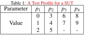
Table 1:A Test Profile for a SUT Parameter p1 p2 p3 p4
Value 01 34 67 89
2 5 -
-Table 1 gives an example of a SUT withD = ∅, in which 52
there are four parameters, two of which have two values and 53
another two of which have three values: the test profile can be 54
written asT P(4,2232,∅). 55
Definition 2. Given a test profile T P(k,|V1||V2| · · · |Vk|,D), a
k-56
tuple(v1,v2,· · · ,vk)is a combinatorial test case for the SUT,
57
where vi∈Vi(i=1,2,· · ·,k).
58
For example, (0,3,6,8) is a 4-tuple combinatorial test case
59
for the SUT shown in Table 1.
60
Definition 3. The number of parameters required to trigger a
61
failure is referred to as the failure-triggering fault interaction
62
(FTFI) number.
63
The combinatorial input domain fault model assumes that
64
failures are caused by parameter interactions. For example, if
65
the SUT shown in Table 1 fails when both p2 is set to 5 and 66
p3is set to 6, this failure is caused by the parameter interaction 67
(p2, p3), and therefore, the FTFI number is 2. 68
In combinatorial interaction testing, a covering array is
69
generally used to represent an interaction test suite.
70
Definition 4. Given a T P(k,|V1||V2| · · · |Vk|,D), an N×k matrix
71
is aτ-wise (1≤τ≤k) covering array, denoted CA(N;τ,k,|V1| 72
|V2| · · · |Vk|), which satisfies the following properties: (1) each
73
column i(i = 1,2,· · ·,k)contains only elements from the set
74
Vi; and (2) the rows of each N×τsub-matrix cover allτ-wise
75
value combinations from theτcolumns at least once. 76
Table 2 shows an example covering array for the SUT in
77
Table 1. The covering array, denoted asCA(9; 2,4,2232), only
78
requires a set of nine test cases in order to cover all 2-wise value
79
combinations.
80
Each column of a covering array represents a parameter of
81
the SUT, while each row represents a combinatorial test case.
82
Testing with a τ-wise covering array is called τ-wise
83
Table 2:CA(9; 2,4,2232) for theT P(4,2232,∅) shown in Table 1
Test No. p1 p2 p3 p4
tc1 0 3 7 9
tc2 0 4 6 8
tc3 0 5 7 8
tc4 1 3 6 9
tc5 1 4 7 8
tc6 1 5 6 9
tc7 2 3 7 8
tc8 2 4 6 9
combinatorial interaction testing. In this paper, we focus on
1
τ-wise covering arrays, rather than on other interaction test
2
suites such asvariable-strength covering array[9].
3
In τ-wise combinatorial interaction testing, theuncovered
4
λ-wise value combinations distance(UVCDλ) is a distance (or
5
dissimilarity) measure often used to evaluate combinatorial test
6
cases against an interaction test suite [20].
7
Definition 5. Given an interaction test suite T, strengthλ, and 8
a combinatorial test case tc, the uncovered λ-wise value 9
combinations distance (UVCDλ) of tc against T is defined as:
10
UVCDλ(tc,T)=|CombSetλ(tc)\CombSetλ(T)|, (1)
where CombSetλ(tc)is the set of allλ-wise value combinations
11
covered by tc, and CombSetλ(T)is the set covered by all of T.
12
More specifically, these can be respectively written as follows:
13
CombSetλ(tc)={(vj1,vj2,· · · ,vjλ)|1≤j1<j2<· · ·<jλ≤k}, (2)
14
CombSetλ(T)=
!
tc∈T
CombSetλ(tc). (3)
In the past, minimization of the interaction test suite size
15
has been emphasized in order to achieve the desired coverage,
16
and although the problem of constructing interaction test suites
17
(covering array and variable-strength covering array) is
18
NP-Complete [35], many strategies for building them have
19
been developed, including approaches employing greedy,
20
recursive, heuristic search, and algebraic algorithms and
21
methods (see [29] for more details).
22
2.2. Test case prioritization
23
SupposeT ={tc1,tc2,· · ·,tcN}is a test suite containingN
24
test cases, and S = ⟨s1,s2,· · ·,sN⟩ is an ordered set of T,
25
called a test sequence, where si ∈ T and
26
si ! sj (i,j =1,2,· · · ,N;i! j). IfS1 =⟨s1,s2,· · ·,sm⟩and
27
S2 =⟨q1,q2,· · ·,qn⟩are two test sequences, we defineS1≻S2 28
as ⟨s1,s2,· · ·, sm,q1,q2,· · · ,qn⟩; and T \S as the maximal
29
subset ofT whose elements are not inS.
30
Test case prioritization is used to schedule test cases in an
31
order, so that, according to some criteria (e.g. condition
32
coverage), test cases with higher priority are executed earlier
33
in the testing process. A well-prioritized test sequence may
34
improve the likelihood of detecting faults earlier, which may
35
be especially important when testing with limited test
36
resources. The problem of test case prioritization is defined as
37
follows [34]:
38
Definition 6. Given(T,Ω,g), where T is a test suite,Ωis the
39
set of all possible test sequences obtained by ordering test cases
40
of T, and g is a function from a given test sequence to an award
41
value, the problem of test case prioritization is to find an S ∈Ω
42
such that:
43
(∀S′) (S′∈Ω) (S′!S) [g(S)≥g(S′)]. (4)
In Eq. (4),gis a function to evaluate a test sequenceS by
44
returning a real number. A well-known function isa weighted
45
average of the percentage of faults detected (APFD) [13],
46
which is a measure of how quickly a test sequence can detect
47
faults during the execution (that is, the rate of fault detection).
48
LetT be a test suite containingNtest cases, and letFbe a set
49
ofmfaults revealed byT. LetSFibe the number of test cases
50
in test sequenceS ofT that are executed until detecting faulti.
51
The APFD for test sequence S is given by the following
52
equation from [13]:
53
APFD=1−SF1+SF2+· · ·+SFm
N×m +
1
2N. (5)
The APFD metric, which has been used in practical
54
testing, has a range of (0,1), with higher values implying faster
55
rates of fault detection. Two requirements of the APFD metric
56
are that (1) all test cases in a test sequence should be executed;
57
and (2) all faults should be detected. In practical testing
58
applications, however, it may be that only part of the test
59
sequence is run, and only some of the faults detected. In such
60
cases, the APFD may not be an appropriate evaluation of the
61
fault detection rate. To alleviate the difficulties associated with
62
these two requirements, Qu et al.[32] have presented a new
63
metric, Normalized APFD (NAPFD), as an enhancement of
64
APFD, and defined it as follows:
65
NAPFD=p−SF1+SF2+· · ·+SFm
N′×m +
p
2N′, (6)
wheremandSFi(i=1,2,· · ·,m) have the same meaning as in
66
APFD;prepresents the ratio of the number of faults identified
67
by selected test cases relative to the number of faults detected
68
by the full test suite; andN′is the number of the executed test 69
cases. If a fault fiis never found, thenSFi=0. If all faults can 70
be detected, and all test cases are executed, NAPFD and APFD
71
are identical, withp=1.0 andN′=N. 72
Many test case prioritization strategies have been
73
proposed, such as fault severity based prioritization [12],
74
source code based prioritization [34, 41], search based
75
prioritization [26], integer linear programming based
76
prioritization [44], XML-manipulating prioritization [28], risk
77
exposure based prioritization [43], system-level test case
78
prioritization [36], and history based prioritization [21]. Most
79
prioritization strategies can be classified as either
80
meta-heuristic search methods or greedy methods [40].
81
3. Related Work 82
According to Qu’s classification, the prioritization of
83
interaction test suites can generally be divided into two
84
categories: (1)pure prioritization: re-ordering test cases in the
85
interaction test suite; and (2) re-generation prioritization:
86
considering the prioritization principle during the process of
87
interaction test suite generation, that is, generating (or
88
constructing) an interaction test sequence [32]. The method
89
proposed in this paper, as well as the methods used for
90
comparison, belongs to the former category. However, if based
91
on the same prioritization principle,pure prioritizationworks
92
in a similar manner to re-generation prioritization. For
example, when testers base prioritization on test case
1
execution time, pure prioritization chooses an element from
2
the given test suite such that it has the lowest execution time,
3
and re-generation prioritization selects (or generates) such
4
elements from the exhaustive test suite (or constructed
5
candidates). In this section, therefore, we do not distinguish
6
betweenpureandre-generationprioritization.
7
Bryce and Colbourn [1, 2] initially used four test case
8
weighting distributions to construct interaction test sequences
9
with seeding and constraints, which belongs to the
10
re-generation prioritization category. Bryce et al. [4, 5]
11
proposed apure prioritizationmethod without considering any
12
other factors (only considering 2-wise and 3-wise interaction
13
coverage) for interaction test suites, and then applied it to the
14
event-driven software. Similarly, Quet al.[31–33] applied test
15
case weight to thepure prioritizationmethod, and applied this
16
method to configurable systems. They also proposed other test
17
case weighting distributions based on code coverage [32],
18
specification [32], fault detection [31], and configuration
19
change [31]. Additionally, Chenet al.[7] used an ant colony
20
algorithm to generate prioritized interaction test suites which
21
considered interaction coverage information.
22
Srikanthet al. [37] took the cost of installing and building
23
new configurations into consideration for helping prioritize
24
interaction test suites. Bryce et al. [6] used the length of the
25
test case to represent its cost, and combined it with pair-wise
26
interaction coverage to guide the prioritization of interaction
27
test suites. Wanget al. [40] combined test case cost with test
28
case weight to prioritize interaction test suites, and also
29
extended this method from lower to higher strengths, and
30
proposed a series of metrics which have been widely used in
31
the evaluation of interaction test sequences. Petke et al. [30]
32
researched the efficiency and fault detection of the pure
33
prioritizationmethod proposed in [4, 5] with other (lower and
34
higher) strengths. Recently, Huang et al. [18] investigated
35
adaptive random test case prioritization for interaction test
36
suites using interaction coverage, a method which, by
37
replacing the prioritization method in [4, 5] attempts to reduce
38
time costs, while maintaining effectiveness.
39
Throughout the interaction test suite prioritization process,
40
the strategies so far mentioned [1, 2, 4–7, 18, 30–33, 37, 40]
41
do not vary the strength of interaction coverage. For example,
42
given a strength τ for prioritization, these prioritization 43
strategies only consider τ-wise interaction coverage to guide
44
the test cases selection. These implementations of
45
“fixed-strength prioritization” are also referred to as
46
interaction coverage based prioritization(or ICBP). Previous
47
studies also investigated incremental strengths to prioritize
48
interaction test suites. For instance, Wang [39] used
49
incremental strengths, and proposed a pure prioritization
50
method named inCTPri used to prioritize covering arrays.
51
More specifically, given a τ-wise covering array
52
CA(N;τ,k,|V1||V2| · · · |Vk|), the inCTPri firstly uses interaction
53
coverage at a low strength (such as λ where 1 < λ ≤ τ) to 54
prioritize CA; when all λ-wise value combinations have been 55
covered by selected test cases, the inCTPri increases λ to 56
λ+1, and then repeats the above process untilλ>τ. In other 57
words, inCTPri is actually ICBP using different strengths
58
during the prioritization process. Huanget al. [19] proposed
59
two pure prioritization methods for variable-strength covering
60
arrays which exploit the main-strength and sub-strengths of
61
variable-strength covering arrays to guide prioritization.
62
To date, most interaction test suite prioritization strategies
63
belong to the category of “fixed-strength prioritization”,
64
because they only consider a fixed strength when selecting
65
each combinatorial test case from candidates. Few studies
66
have been conducted on the prioritization of interaction test
67
suites using “aggregate-strength prioritization”, and our study
68
is, to our best knowledge, the first to use multiple strengths
69
when choosing each combinatorial test case from the candidate
70
elements.
71
4. Aggregate-Strength Interaction Test Suite Prioritization 72
In this section, we present a motivating example to
73
illustrate the shortcoming of “fixed-strength prioritization”,
74
and then introduce a new dissimilarity measure for evaluating
75
combinatorial test cases, theweighted aggregate-strength test
76
case dissimilarity (WASD). We then introduce a heuristic
77
algorithm for prioritizing an interaction test suitebased on the 78
WASDmeasure(“aggregate-strength prioritization” strategy),
79
investigate some of its properties, and give a time complexity
80
analysis.
81
4.1. A motivating example
82
Given covering arrayCA(9; 2,4,2232), shown in Table 2, 83
“fixed-strength prioritization” generally uses strengthτ=2 to 84
guide the prioritization. More specifically, this strategy
85
chooses the next test case such that it covers the largest
86
number of 2-wise value combinations that have not yet been
87
covered by the already selected test cases (that is, UVCD2). 88
We assume that “fixed-strength prioritization” is deterministic,
89
e.g. the first candidate is selected as the next test case in
90
situations with more than one best element, and therefore its
91
generated interaction test sequence would be
92
S1 = ⟨tc1,tc2,tc6,tc5,tc7,tc8,tc3,tc4,tc9⟩. Intuitively 93
speaking, S1 would face a challenge when a fault f1 is 94
triggered by “P1=2”, because it needs to run five test cases 95
(5/9 = 55.56%) in order to detect this fault. However, if
96
multiple strengths were used to prioritize this interaction test
97
suite, e.g. strengths 1 and 2, both 1-wise and 2-wise value
98
combinations would be considered, and therefore we would
99
obtain the interaction test sequence
100
S2 = ⟨tc1,tc9,tc4,tc2,tc5,tc7,tc8,tc3,tc6⟩. S2 would only 101
require 2 test cases (2/9 = 22.22%) to be run to identify the
102
fault f1, which means thatS2 has a faster fault detection than 103
S1. 104
Motivated by this, it is reasonable to consider different
105
strengths for prioritizing interaction test suites, which may
106
provide better effectiveness (such as fault detection) than
107
“fixed-strength prioritization”.
4.2. Weighted aggregate-strength test case dissimilarity
1
Given an interaction test suite T on
2
T P(k,|V1||V2| · · · |Vk|,D), a combinatorial test case tc, and the
3
strength τ, the weighted aggregate-strength test case 4
dissimilarity(WASD) oftcagainstT is defined as follows:
5
WASD(tc,T)=
τ
"
λ=1
(ωλ×|UVCDλ(tc ,T)|
Cλ k
), (7)
where 0≤ωλ≤1.0 (λ=1,2,· · ·,τ), and#τλ=1ωλ=1.0.
6
Intuitively speaking,WASD(tc,T)=0, if and only iftc∈T; 7
WASD(tc,T)=1.0, if and only if any 1-wise value combination
8
covered bytcis not covered byT. Therefore, theWASDranges
9
from 0 to 1.0.
10
Here, we present an example to briefly illustrate theWASD.
11
Considering the combinatorial test cases in Table 2, suppose
12
interaction test sequence S = {tc1}, strength τ = 2, two 13
candidates tc2 andtc9, andω1 = ω2 = · · · = ωτ = 1/τ, the
14
WASD of tc2 against T is
15
WASD(tc2,S) = 12 × UVCDλC=11(tc2,S)
4 +
1
2 × UVCDλC=22(tc2,S)
4 =
16 1
2 ×34 +12 ×66 =0.375+0.5 =0.875; while theWASDoftc9 17
against S is
18
WASD(tc9,S) = 12 × UVCDλC=11(tc9,S) 4
+ 12 × UVCDλ=2(tc9,S)
C2 4
= 19
1
2 × 44 + 12 × 66 = 0.5+0.5 = 1.0. In this case, it can be 20
concluded that the test casetc9would be a better next test case 21
inS thantc2. 22
4.3. Algorithm
23
In this section, we introduce a new heuristic algorithm,
24
namely “aggregate-strength prioritization” strategy (ASPS), to
25
Algorithm 1Aggregate-strength prioritization strategy (ASPS)
Input: Covering arrayCA(N;τ,k,|V1||V2| · · · |Vk|), denoted as Tτ
Output: Interaction test sequenceS
1: S ← ⟨ ⟩;
2: while(|S|!N)
3: best distance← −1;
4: equalSet←{ };
5: for(each elemente∈Tτ)
6: Calculatedistance←WASD(e,S);
7: if(distance>best distance)
8: equalSet←{ };
9: best distance←distance;
10: best data←e;
11: else if(distance==best distance) 12: equalSet←equalSet${e}; 13: end if
14: end for
15: best data←random(equalSet);
16: /* Randomly choose an element fromequalSet*/ 17: Tτ←Tτ\ {best data};
18: S ←S≻⟨best data⟩;
19: end while 20: return S.
prioritize interaction test suites using the WASD to evaluate
26
combinatorial test cases.
27
Given a covering arrayT =CA(N;τ,k,|V1||V2| · · · |Vk|), the
28
element e′ is selected from T as the next test element in an 29
interaction test sequenceS when using theWASD, such that:
30
(∀e) (e∈T) (e!e′) [WASD(e′,S)≥WASD(e,S)]. (8)
This process is repeated until all candidates have been selected.
31
The ASPS algorithm is described in Algorithm 1. In some
32
cases, there may be more than one best test element, indicating
33
that they have the same maximal WASD value. In such a
34
situation, a best element is randomly selected.
35
For ease of description, we use a term Tτ to represent a
36
CA(N;τ,k,|V1||V2| · · · |Vk|), with the strength τ used in the
37
WASDand Algorithm 1 often being provided by a CA rather
38
than being assigned in advance.
39
4.4. Properties
40
Consider a Tτand a pre-selected interaction test sequence
41
S ⊆Tτprioritized by the ASPS algorithm, some properties of
42
ASPS are discussed as follows.
43
Theorem 1. Once S covers all possible (τ−1)-wise value
44
combinations where2 ≤ τ ≤ k, the ASPS algorithm has the
45
same mechanism as the “fixed-strength prioritization
46
strategy”.
47
Proof. When S covers all possible (τ − 1)-wise value
48
combinations, it can be noted that
49
CombSetτ−1(S)=CombSetτ−1(Tτ), which means that
50
(∀tc) (tc∈(Tτ\S)) [UVCDτ−1(tc,S)=0]. (9)
Since
51
CombSetτ−1(S)=CombSetτ−1(Tτ)
⇒ CombSetλ(CombSetτ−1(S))=CombSetλ(CombSetτ−1(Tτ))
⇒ CombSetλ(S)=CombSetλ(Tτ), (10)
where 1≤λ≤τ−1. Therefore, we can obtain that
52
(∀tc) (tc∈(Tτ\S)) [UVCDλ(tc,S)=0]. (11)
where λ = 1,2,· · ·,τ − 1. As a consequence,
53
WASD(tc,S) = ωτ × UVCDτCτ(tc,S)
k . Since ωτ is a constant
54
parameter, WASD(tc, S) is only related to UVCDτ(tc,S).
55
Consequently, the ASPS algorithm only uses τ-wise
56
interaction coverage to select the next test case, which means
57
that it is “fixed-strength prioritization”. In summary, onceS
58
covers all possible (τ−1)-wise value combinations, the ASPS
59
algorithm becomes the same as “fixed-strength
60
prioritization”.
61
4.5. Complexity analysis
62
In this section, we briefly analyze the complexity of the
63
ASPS algorithm (Algorithm 1). Given aCA(N;τ,k,|V1||V2| · · · 64
|Vk|), denoted asTτ, we defineδ=max1≤i≤k{|Vi|}.
We first analyze the time complexity of selecting thei-th
1
(i = 1,2,· · ·,N) combinatorial test case, which depends on
2
two factors: (1) the number of candidates required for the
3
calculation of WASD; and (2) the time complexity of
4
calculatingWASDfor each candidate.
5
For (1), (N−i)+1 test cases are required to computeWASD. 6
For (2), according toCl
kl-wise parameter combinations where
7
1 ≤ l ≤ τ, we divide all l-wise value combinations that are 8
derived from aT P(k,|V1||V2| · · · |Vk|,D) intoClksets that form
9
Πl={πl|πl={(vi1,vi2,· · ·,vil)|vij ∈Vij,j=1,2,· · · ,l},
1≤i1<i2<· · ·<il≤k}. (12)
Consequently, when using a binary search, the order of time
10
complexity of (2) isO(#τ
l=1#πl∈Πllog(|πl\CombSetl(T)|)),
wh-11
ich is equal toO(#τ
l=1#πl∈Πllog(|πl|)).
12
Therefore, the order of time complexity of algorithm ASPS
13
can be described as follows:
14
O(ASPS)=O((
N
"
i=1
(N−i+1))×(
τ
"
l=1
"
πl∈Πl
log(|πl|)))
<O(( N
"
i=1
(N−i+1))×
τ
"
l=1
(Cl
k×log(δl)))
=O(N 2+N
2 ×
τ
"
l=1
(Cl
k×log(δl))). (13)
There exists an integerη(1≤η≤τ) such that2: 15
(∀l) (1≤l≤τ) (η!l) [(Cη
k×log(δη))≥(Clk×log(δl))]. (14)
As a consequence,
16
O(ASPS)<O(N2+N
2 ×
τ
"
l=1
(Cη
k×log(δη)))
=O(N 2+N
2 ×τ×C
η
k×log(δη)) (15)
Therefore, we can conclude that the order of time complexity
17
of algorithm ASPS isO(N2×τ×Cη
k×log(δη)).
18
The value ofτis usually assigned in the range from 2 to 6
19
[23, 24], therefore, 1 ≤ τ < ⌈k
2⌉, in general. If 1 ≤τ <⌈k2⌉, 20
η =τ, then the order of time complexity of algorithm ASPS is
21
O(τ×N2×Cτ
k×log(δτ)). Since counting the number of value
22
combinations at different strengths can be implemented in
23
parallel, the order of time complexity of the ASPS algorithm
24
can be reduced toO(N2×Cτ
k×log(δτ)). As discussed in [40],
25
the order of time complexity of the ICBP algorithm (an
26
implementation of “fixed-strength prioritization”) is
27
O(N2 ×Cτ
k ×log(δτ)). The order of time complexity of the
28
inCTPri algorithm (another “fixed-strength prioritization”
29
implementation) also equals to O(N2 × Cτ
k ×log(δτ)) [39].
30
Therefore, the order of time complexity of the ASPS algorithm
31
is similar to that of both ICBP and inCTPri.
32
2If 1≤τ<⌈k
2⌉,η=τ; while if⌈k2⌉ ≤τ≤k,η=⌈k2⌉.
5. Empirical Study 33
In this section, some experimental results, including
34
simulations and experiments involving real programs, are
35
presented to analyze the effectiveness of the prioritization of
36
interaction test suites by multiple interaction coverage
37
(multiple strengths). We evaluate interaction test sequences
38
prioritized by algorithm ASPS (denotedASPS) by comparing
39
them with those ordered by four other strategies: (1)
40
test-case-generation prioritization (denotedOriginal), which
41
is an interaction test sequence according to the covering array
42
generation sequence; (2) reverse test-case-generation
43
prioritization (denoted Reverse), which is the reversed order
44
of the Original interaction test sequence; (3) random test
45
sequence, whose ordering is prioritized in a random manner
46
(denoted Random); and (4) two implementations of
47
“fixed-strength prioritization” – the ICBP algorithm (denoted
48
ICBP) [1, 2, 4–7, 18, 30–33, 37, 40]; and the inCTPri
49
algorithm (denotedinCTPri) [39].
50
In Algorithm 1, which usesWASD, it is necessary to assign
51
a weight for each interaction coverage (Eq. (7)). The ideal
52
weight assignment is in accordance with actual fault
53
distribution in terms of the FTFI number. However, the actual
54
fault distribution is unknown before testing. In this paper, we
55
focus on three distribution styles: (1) equal weighting
56
distribution – each interaction coverage has the same weight,
57
that is, ω1 = ω2 = · · · = ωτ = 1τ; (2) random weighting
58
distribution – the weight of each interaction coverage is
59
randomly distributed; and (3) empirical FTFI percentage
60
weighting distribution based on previous investigations
61
[23, 24]: for example, in [24], several software projects were
62
studied and the interaction faults reported to have 29% to 82%
63
faults as 1-wise faults, 6% to 47% of faults as 2-wise faults,
64
2% to 19% as 3-wise faults, 1% to 7% of faults as 4-wise
65
faults, and even fewer faults beyond 4-wise interactions.
66
Consequently, we arranged the weights as follows:
67
ω1=ω,ωi+1 =12ωi, wherei=1,2,· · · ,τ−1. For example, if
68
τ =2, we setω1 = 0.67 andω2 =0.33; ifτ =3,ω1 =0.57,
69
ω2 = 0.29, andω3 = 0.14. For clarity of description, we use
70
ASPSe, ASPSr, and ASPSm to represent the ASPS algorithm
71
with equal weighting distribution, random weighting
72
distribution, and empirical FTFI percentage weighting
73
distribution, respectively.
74
The original covering arrays were generated using two 75
popular tools: (1) Advanced Combinatorial Testing System 76
(ACTS) [25, 38]; and (2)Pairwise Independent Combinatorial 77
Testing(PICT) [10]. Both ACTS and PICT are supported by 78
greedy algorithms, however, they are implemented by different
79
strategies: ACTS is implemented by the In-Parameter-Order 80
(IPO) method [38]; while PICT is implemented by the 81
one-test-at-a-time approach [3]. We focused on covering
82
arrays with strengthτ = 2,3,4,5. We designed simulations
83
and experiments to answer the following research questions:
84
RQ1: Do prioritized interaction test sequences generated
85
by ASPS methods (ASPSe, ASPSr, and ASPSm) have better
86
performance (e.g. fault detection) when compared with
87
non-prioritized interaction test suites (Original)? The answer
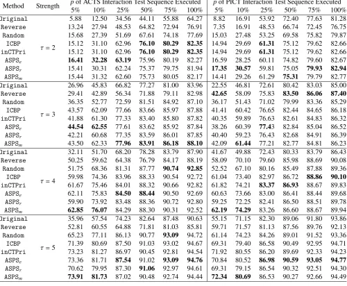
Table 3: Sizes of covering arrays for four test profiles.
Test Profile ACTS PICT
τ=2 τ=3 τ=4 τ=5 τ=2 τ=3 τ=4 τ=5
T P1(6,56,∅) 25 199 1058 4149 37 215 1072 4295
T P2(10,23334351,∅) 23 103 426 1559 23 109 411 1363
T P3(7,243161161,∅) 96 289 578 1728 96 293 744 1658
T P4(8,2691101,∅) 90 180 632 1080 90 192 592 1237
to this question will help us decide whether it would be
1
necessary to prioritize interaction test suites using ASPS
2
methods.
3
RQ2: Are ASPS methods better than intuitive
4
prioritization strategies such as the reverse prioritization
5
(Reverse) and the random prioritization (Random)? The
6
answer to this question will tell us whether or not it would be
7
helpful to use ASPS methods rather than reverse or random
8
ordering for prioritizing interaction test suites.
9
RQ3: Do ASPS methods perform better than
10
“fixed-strength prioritization” (ICBP and inCTPri)? The
11
answer to this question will help us decide whether or not
12
ASPS can be a promising technique for interaction test suite
13
prioritization, especially if it could perform as effectively as
14
the current best prioritization techniques (“fixed-strength
15
prioritization”).
16
RQ4: Which weighting distribution is more suitable for
17
the ASPS method: equal weighting distribution, random
18
weighting distribution, or empirical FTFI percentage
19
weighting distribution? The answer to this question will help
20
us decide which weighting distribution to use for the ASPS
21
method.
22
5.1. Simulation
23
We ran a simulation to measure how quickly an interaction
24
test sequence could cover value combinations of different
25
strengths. The simulation details are presented in the
26
following.
27
5.1.1. Setup
28
We designed four test profiles as four system models with
29
details as shown in Table 3. The first two test profiles were
30
T P1(6,56,∅) and T P2(10,23334351,∅), both of which have
31
been used in previous studies [40]. The third and fourth test 32
profiles (T P3(7,243161161,∅) and T P4(8,2691101,∅)) have 33
previously been created [32, 33] to model real-world subjects 34
– a module from a lexical analyzer system (flex), and a real 35
configuration model for GNUzip (gzip)3. 36
The sizes of the covering arrays generated by ACTS and
37
PICT are given in Table 3, Since randomization is used in some
38
test case prioritization techniques, we ran each test profile 100
39
times and report the average of the results.
40
3These two models are unconstrained and incomplete.
5.1.2. Metric
41
The average percentage of combinatorial coverage
42
(APCC) metric4 [40] is used to evaluate the rate of value 43
combinations covered by an interaction test sequence. The
44
APCC values range from 0% to 100%, with higher values
45
meaning better rates of covering value combinations. Let an
46
interaction test sequenceS = ⟨s1,s2,· · ·,sN⟩be obtained by
47
prioritizing a CA(N;τ,k,|V1||V2| · · · |Vk|), that is, Tτ, the
48
formula to calculate APCC at strengthλ(1≤λ≤τ) is: 49
APCCλ(S)=
#N−1
i=1 |$ij=1CombSetλ(sj)| N×|CombSetλ(Tτ)| ×
100%. (16)
50
Additionally, since we consider λ = 1,2,· · ·,τ for an 51
interaction test sequenceS of aCA(N;τ,k,|V1||V2| · · · |Vk|), we
52
could obtain τAPCC values (that is, APCC1(S), APCC2(S), 53
· · ·, APCCτ(S)). Therefore, in this simulation we also
54
considered the average of the APCC values, which is defined
55
as:
56
Avg.(S)= 1 τ
τ
"
λ=1
APCCλ(S). (17)
5.1.3. Results and Discussion
57
For covering arrays of strengthτ(2≤τ≤5) on individual
58
test profiles, we have the following observations based on the
59
data in Tables 4 and 5, which are separated according to the
60
four test profiles.
61
1) According to the APCC metric, are prioritized
62
interaction test suites by ASPS methods better than
63
non-prioritized interaction test suites? In this part, we analyze
64
the data to answer whether ASPS methods (ASPSe,ASPSr, and
65
ASPSm) are more effective thanOriginal.
66
Since different weighting distributions in ASPS provide
67
different APCC values, we compare the APCC values of each
68
ASPS method with Original. In 98.21% (110/112), 69
86.61% (97/112), and 98.21% (110/112) of cases, interaction 70
test sequences prioritized by ASPSe, ASPSr, and ASPSm,
71
4In [30], Petke et al. proposed a similar metric, namely the average percentage of covering-array coveragemetric (APCC). Both Wang’s APCC [40] and Petke’s APCC [30] aim at measuring how quickly an interaction test sequence achieves interaction coverage at a given strength. In fact, their APCCs are equivalent: given two interaction test sequences,S1andS2, if one
determines that the test sequenceS1is better thanS2, then the other metric will
also have the same determination. The only difference between them is that they
use different plot curves to describe the rate of covered value combinations.
Table 4: APCC λ metric (%) for di ff erent prioritization techniques for TP 1(6 , 5
6,∅
)and TP 2(10 , 2 33 34 35 1,∅
Table 5: APCC λ metric (%) for di ff erent prioritization techniques for TP 3(7 , 2 43 16 116 1,∅
)and TP 4(8 , 2 69 110 1,∅
respectively, have greater APCC values than Original test 1
sequences. Additionally, the average APCC values of ASPSe,
2
ASPSr, and ASPSm are higher than those of Original, in
3
100.00% (32/32), 84.38% (27/32), and 100.00% (32/32) of 4
cases, respectively. 5
As shown in Tables 4 and 5, it can be noted that different
6
non-prioritized interaction test suites generated by different
7
tools have different performances.
8
For example, consider T P3(7,243161161,∅) at strength
9
τ = 2: when non-prioritized covering arrays are constructed 10
using ACTS, the difference betweenASPSe andOriginalis
11
18.60% for λ = 1, and 32.31% forλ = 2. However, when 12
using PICT, the difference is 1.79% forλ= 1, and 1.74% for 13
λ = 2. The main reason for this is related to the different 14
mechanisms used in the ACTS and PICT tools [10, 25, 38].
15
Specifically, without loss of generality, consider a test profile 16
T P(k,|V1||V2| · · · |Vk|,∅) with|V1| ≥ |V2| ≥ · · · ≥ |Vk|. When
17
generating a τ-wise (1 ≤ τ ≤ k) covering array, the ACTS 18
algorithm first uses horizontal growth[25, 38] to construct a 19
τ-wise test set for the firstτparameters, which implies that it 20
needs at least (1+(|V1|−1)×%τi=2|Vi|) test cases to cover all
21
possible 1-wise value combinations. However, the PICT 22
algorithm chooses each next test case such that it covers the 23
largest number ofτ-wise value combinations that have not yet
24
been covered – a mechanism similar to that ofICBP. 25
In conclusion, the simulation indicates that the ASPS
26
techniques do outperform Original in terms of the rate of
27
covering value combinations, regardless of which construction
28
tools are used (ACTS or PICT).
29
2) Do ASPS methods have better APCC values than
30
reverse or random ordering? In this part, we attempt to
31
determine whether or not ASPS methods are more effective
32
than two widely-used prioritization methods, Reverse and
33
Random.
34
In all cases, each ASPS method (regardless of ASPSe,
35
ASPSr, and ASPSm) has higher APCC values than Reverse,
36
and hence achieves higher average APCC values. Additionally,
37
the performance of Reverse is correlated with the
38
non-prioritized interaction test suite (that is, the ACTS and
39
PICT tools).
40
Compared with Random, the ASPS methods have higher
41
APCC values in all cases, irrespective of the strength
42
λ = 1,2,· · ·,τ and interaction test suite construction tool 43
(ACTS or PICT). As a result, the ASPS methods have better
44
performance according to the average APCC values at
45
different strengths.
46
In conclusion, in all casesour ASPS methods (regardless
47
of the weighting distributions) do perform better than both the
48
ReverseandRandomprioritization strategies, according to the
49
APCC values.
50
3) Are ASPS methods better than “fixed-strength
51
prioritization”? In this part, we would like to determine
52
whether or not ASPS methods perform better than two
53
implementations of “fixed-strength prioritization”, ICBP and
54
inCTPri.
55
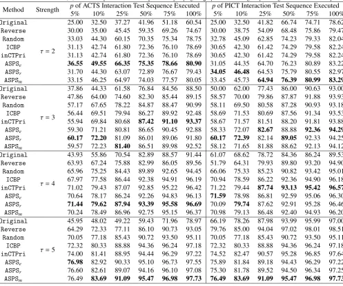
Compared with ICBP, according to APCC values,ASPSe,
56
ASPSr and ASPSm perform better in 79.46% (89/112),
57
ASPSe: 33.63%
ASPSm: 65.77%
ASPS
r
: 0
.6
[image:10.595.338.523.81.195.2]%
Figure 1: Comparison ofASPSe,ASPSr, andASPSmaccording to APCC.
36.61% (41/112), and 72.32% (81/112) of cases, respectively.
58
Furthermore, according to the average of APCC values (Avg.), 59
ASPSe,ASPSr, andASPSmhave better performances thanICBP
60
in 100.00% (32/32), 18.75% (6/32), and 100.00% (32/32) of 61
cases. 62
Similarly, compared with inCTPri, ASPSe, ASPSr, and
63
ASPSm have higher APCC values in 58.93% (66/112),
64
21.43% (24/112), and 75.00% (84/112) of cases, respectively. 65
Moreover, according to the average of APCC values, ASPSe,
66
ASPSr, and ASPSm outperforminCTPri in 100.00% (32/32),
67
3.13% (1/32), and 100.00% (32/32) of cases.
68
In conclusion, the simulation results indicate that apart 69
from ASPSr, in (58.93% ∼ 79.46%) of cases our ASPS
70
methods (ASPSeandASPSm) do perform better thanICBPand
71
inCTPri, and also have higher averages of APCC values in all 72
cases. Consequently, we conclude that our ASPS methods 73
(except for ASPSr) do have better performance than
74
“fixed-strength prioritization”. 75
4) Among the three weighting distributions, which
76
weighting distribution is used for the ASPS method? In this
77
part, we are interested in which weighting distribution is more
78
suitable for the ASPS method. As discussed before, there are
79
three distributions used for the ASPS methods: equal, random,
80
and empirical FTFI percentage weighting distributions.
81
As discussed in the last part, among the three weight
82
distributions for ASPS, ASPSr has the lowest APCCλ
83
performance, irrespective of whichλvalue is used (1≤λ≤τ). 84
Additionally, when λ is high, ASPSe performs better than
85
ASPSm, otherwise it performs worse. According to the average
86
APCC values, however, ASPSm performs best, followed by
87
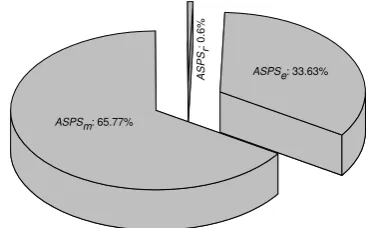
ASPSe; while ASPSr has the worst performance. Figure 1
88
shows the comparison of ASPSe,ASPSr, andASPSmaccording
89
to the APCC metric. From this figure, it can be observed that 90
in 65.77% (73.67/112) of casesASPSmhas the highest APCC
91
values; in 33.63% (37.67/112) of cases,ASPSedoes; and only
92
in 0.60% (0.67/112) of cases is the highest values forASPSr5.
93
In other words, among three weighting distributions, empirical 94
FTFI percentage weighting distribution would be the best 95
choice, followed by the equal weighting distribution, 96
according to the APCC metric. 97
Table 6: Subject programs.
Subject Program Test Profile #uLOC #Seeded Faults #Detectable Faults #Used Faults
count T P(6,2135,∅) 42 15 12 12
nametbl T P(5,213252,∅) 329 51 44 43
flex T P(9,263251,D), 9,581∼11,470 81 50 34
grep T P(9,213342516181,D) 9,493∼10,173 57 12 10
In conclusion, the empirical FTFI percentage weighting
1
distribution appears to be more suitable than the other
2
weighting distributions for the ASPS method (ASPSm).
3
5) Conclusion: Based on the above discussions, we find
4
that given a covering array of strengthτ, theASPS strategies
5
behave better than the Original, Reverse, and Random
6
strategies (in 86.61% ∼ 100.00% of cases), and apart from
7
ASPSr perform better than “fixed-strength prioritization”
8
including ICBP and inCTPri implementations (in
9
58.93% ∼ 79.46% of cases). Additionally, among the three
10
weighting distributions, the empirical FTFI percentage is most
11
suitable for use with the ASPS method, followed by the equal
12
weighting distribution.
13
5.2. Experiments
14
An experimental study was also conducted to evaluate the
15
ASPS techniques, the goal of which was to compare the fault
16
detection rates of the ASPSe, ASPSr, and ASPSm techniques
17
against those of other interaction test suite prioritization
18
techniques, such asOriginal,Reverse,Random,ICBP, and
19
inCTPri. In actual testing conditions, testing resources may
20
be limited, and hence only part of an interaction test suite (or
21
an interaction test sequence) may be executed. As a
22
consequence, in this study we focused on different budgets by
23
following the practice adopted in previous prioritization
24
studies [30] of considering different percentages (p) of each
25
interaction test sequence, e.g. p=5%, 10%, 25%, 50%, 75%, 26
and 100% of each interaction test sequence being executed.
27
5.2.1. Setup
28
For the study, we used two small-sized faulty C programs
29
(count and nametbl)6, which had previously been used in 30
research comparing defect revealing mechanisms [27],
31
evaluating different combination strategies for test case
32
selection [17], and fault diagnosis [16, 45]. Since these two
33
programs are small, we also used another two medium-sized
34
UNIX utility programs7, flexandgrep, with real and seeded 35
6Fromhttp://www.maultech.com/chrislott/work/exp/ 7Fromhttp://sir.unl.edu
faults from the Software-artifact Infrastructure Repository
36
(SIR) [11]. These two programs had also been widely used in
37
prioritization research [22, 30, 32]. To determine the
38
correctness of an executing test case, we created a fault-free
39
version of each program (i.e. an oracle) by analyzing the
40
corresponding fault description. These subject programs are
41
described in Table 6, in which theTest Profileis the test profile
42
of each subject program8; the #uLOC9 gives the number of 43
lines of executable code in each program; the #Seeded Faults10 44
is the number of faults seeded in each program; the
45
#Detectable Faults is the number of faults that could be
46
detected from the accompanying test profiles, which are not
47
guaranteed to be able to detect all faults; and the #Used Faults
48
is the number of faults used in the experiment by removing
49
some faults that could be triggered by nearly every
50
combinatorial test case in the test suite,that is, faults could be 51
removed such that they are identified by more than 52
(78.00%∼100.00%) test cases in the test suite. 53
Similar to the simulation (Section 5.1), we also used ACTS
54
and PICT to generate original interaction test sequences for
55
each subject program. Additionally, we focused on covering
56
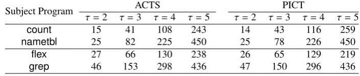
arrays with strengthτ=2,3,4,5. Table 7 gives the sizes of the
57
original interaction test sequences obtained by ACTS and
58
PICT. Because of the randomization in some of the
59
prioritization techniques, we ran the experiment 100 times for
60
each subject program and report the average.
61
5.2.2. Metric
62
The APFD metric [13] is a popular measure for evaluating 63
fault detection rates of interaction test sequence. In this study, 64
only part of the interaction test sequences could be run, and 65
some faults might not have been triggered by a particular 66
interaction test sequence. As discussed before, however, 67
8The test profiles of two medium-sized programs,flexandgrep, are from Petkeet al.[30].
9We used the line count tool named cloc, downloaded from
http://cloc.sourceforge.net, to count the number of code lines.
10Similar to [30], in this study we only used the faults provided with each of subject programs, in order to avoid experiment bias and ensure repeatability.
Table 7: Sizes of original interaction test sequences for each subject program.
Subject Program ACTS PICT
τ=2 τ=3 τ=4 τ=5 τ=2 τ=3 τ=4 τ=5
count 15 41 108 243 14 43 116 259
nametbl 25 82 225 450 25 78 226 450
flex 27 66 130 238 26 65 129 219
[image:11.595.118.471.688.763.2]APFD has two requirements which may cause APFD to fail. 1
Consequently, it was not possible to use APFD to investigate 2
the fault detection rates of the different prioritization strategies,
3
and so we used an enhanced version of APFD, NAPFD [32], 4
as an alternative evaluation metric. 5
5.2.3. Results and Discussions
6
The experimental results from executing all prioritization
7
techniques to test count, nametbl, flex, and grep are
8
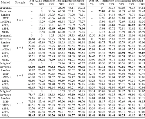
summarized in Tables 8∼11, based on which we can have the
9
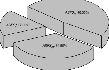
following observations. It should be noted that the data in bold
10
in the tables is the largest in each sub-column.
11
1) Does the ASPS method have faster fault detection rates
12
than the Original method? In this part, we analyze the
13
experimental data to answer the research question of whether
14
or not the ASPS method is better thanOriginalaccording to
15
fault detection rates.
16
As shown in Tables 8 ∼ 11, in 96.84% (184/190),
17
97.37% (185/190), and 96.84% (184/190) of cases, ASPSe,
18
ASPSr, and ASPSm, respectively, obtain interaction test
19
sequences with higher fault detection rates than Original. 20
The fault detection improvement of ASPS overOriginalfor
21
ACTS is larger than that for PICT: as was the case in the
22
simulation, the main reason for this is the different methods
23
used to construct ACTS and PICT interaction test suites.
24
Additionally, as the proportion of the interaction test
25
sequence executed (p) increases, the NAPFD improvement of
26
ASPS over Original generally becomes smaller. For
27
example, consider subject program nametbl for ACTS with
28
τ = 5, when p = 5%, 10%, 25%, 50%, 75%, and 100%, the 29
corresponding NAPFD improvements of ASPSe over
30
Originalare 58.92%, 42.87%, 27.78%, 14.54%, 9.71%, and
31
7.27%, respectively.
32
In conclusion, in (97.37% ∼ 96.84%) of cases, the ASPS 33
method has higher rates of fault detection compared with 34
Original. Furthermore, the ASPS method favors the cases
35
where smaller percentages of interaction test sequence are
36
executed, compared withOriginal.
[image:12.595.47.547.355.766.2]37
Table 8: The NAPFD metric (%) for different prioritization techniques for subject programcountwhen executing the percentage of interaction test sequence.
Method Strength p5%of ACTS Interaction Test Sequence Executed10% 25% 50% 75% 100% p5%of PICT Interaction Test Sequence Executed10% 25% 50% 75% 100%
Original
τ=2
– 0 0 25.00 48.11 59.72 – 0 33.33 69.05 78.33 84.52
Reverse – 0 30.56 62.50 73.11 78.06 – 25.00 43.06 51.79 60.00 71.43
Random – 15.38 37.75 60.08 70.76 76.31 – 17.71 44.18 68.19 76.71 83.21
ICBP – 16.29 40.56 61.98 72.05 77.27 – 17.96 46.67 72.69 80.82 86.30
inCTPri – 16.29 40.56 61.98 72.05 77.27 – 17.96 46.67 72.69 80.82 86.30
ASPSe – 15.21 38.81 62.32 72.09 77.29 – 19.04 50.68 75.45 82.82 87.73
ASPSr – 17.83 42.69 63.86 73.18 78.10 – 17.08 47.72 72.81 80.62 86.15
ASPSm – 13.58 39.10 62.90 72.32 77.45 – 17.13 47.24 73.99 81.79 86.99
Original
τ=3
0 0 1.25 31.04 53.33 65.85 12.50 34.38 65.00 83.33 89.06 91.86
Reverse 39.58 48.96 58.75 74.58 83.06 87.60 0 21.88 55.83 78.97 86.20 89.73 Random 30.40 47.89 71.23 84.03 89.08 91.98 29.96 46.75 71.65 85.79 90.67 93.06
ICBP 29.06 48.25 73.25 86.03 90.64 93.15 27.25 48.43 75.91 88.49 92.45 94.38
inCTPri 31.71 51.96 75.85 87.05 91.34 93.66 32.98 54.44 78.45 89.68 93.23 94.96
ASPSe 32.63 54.40 75.98 86.83 91.16 93.53 30.92 54.42 78.92 89.90 93.37 95.07
ASPSr 33.21 53.60 75.45 86.68 91.09 93.48 34.42 53.15 77.06 88.74 92.61 94.50
ASPSm 35.00 55.78 76.39 86.94 91.23 93.58 30.90 54.75 78.74 89.85 93.34 95.04
Original
τ=4
0 0 0 28.86 51.03 63.27 60.83 80.30 92.53 96.26 97.51 98.13
Reverse 65.00 82.50 93.52 96.76 97.84 98.38 74.17 87.12 95.11 97.56 98.37 98.78 Random 57.02 73.14 89.02 94.48 96.32 97.24 52.12 72.47 88.98 94.49 96.33 97.25
ICBP 56.04 74.30 90.15 95.08 96.72 97.54 52.76 74.07 89.96 94.98 96.65 97.49
inCTPri 60.20 77.81 91.52 95.76 97.17 97.88 59.88 79.42 92.04 96.02 97.35 98.01
ASPSe 61.80 78.25 91.78 95.89 97.26 97.95 60.28 79.11 91.94 95.97 97.31 97.99
ASPSr 60.67 77.70 91.40 95.69 97.13 97.85 60.85 78.61 91.41 95.71 97.14 97.85
ASPSm 61.63 78.34 91.64 95.82 97.21 97.91 60.39 79.32 91.94 95.97 97.31 97.98
Original
τ=5
0 0 0 16.53 35.92 51.75 70.14 85.67 94.40 97.22 98.15 98.62
Reverse 78.47 82.81 88.13 92.63 95.10 96.33 80.56 90.67 96.35 98.19 98.80 99.10 Random 74.65 86.21 94.37 97.21 98.14 98.61 74.84 86.84 94.77 97.41 98.28 98.71
ICBP 76.34 87.46 94.97 97.50 98.34 98.76 76.84 88.17 95.34 97.69 98.46 98.85
inCTPri 80.51 90.08 96.03 98.03 98.69 99.02 81.19 90.77 96.40 98.21 98.81 99.11
ASPSe 80.76 90.27 96.11 98.07 98.72 99.04 80.39 90.41 96.25 98.14 98.76 99.07
ASPSr 79.89 89.48 95.79 97.91 98.61 98.96 80.34 90.27 96.20 98.11 98.75 99.06
Table 9: The NAPFD metric (%) for different prioritization techniques for subject programnametblwhen executing the percentage of interaction test sequence.
Method Strength p5%of ACTS Interaction Test Sequence Executed10% 25% 50% 75% 100% p5%of PICT Interaction Test Sequence Executed10% 25% 50% 75% 100%
Original
τ=2
0 15.70 55.04 75.87 83.91 88.42 11.63 27.33 58.72 72.97 81.98 87.02
Reverse 37.21 57.56 81.78 90.02 93.35 95.21 11.63 23.84 61.43 79.36 86.24 90.09 Random 18.22 32.92 62.85 79.31 86.15 90.03 19.13 33.58 61.53 77.54 84.65 88.91
ICBP 19.15 34.49 68.01 83.55 89.04 92.11 18.92 33.98 65.27 80.48 86.90 90.57
inCTPri 19.15 34.49 68.01 83.55 89.04 92.11 18.92 33.98 65.27 80.48 86.90 90.57
ASPSe 19.38 35.81 69.56 84.33 89.55 92.48 19.21 34.52 66.05 81.31 87.50 91.00
ASPSr 18.21 34.21 67.28 83.06 88.71 91.87 19.23 34.35 64.69 80.26 86.72 90.44
ASPSm 19.57 35.80 68.70 83.89 89.26 92.27 18.99 35.07 67.22 82.28 88.14 91.46
Original
τ=3
27.03 48.55 69.19 84.37 89.50 92.19 40.31 64.12 85.37 92.87 95.21 96.44
Reverse 72.38 82.99 91.63 95.77 97.16 97.89 18.60 53.16 82.19 91.32 94.17 95.66 Random 53.44 71.53 87.80 94.04 96.00 97.02 43.26 66.39 85.87 93.06 95.34 96.53
ICBP 53.77 72.93 88.91 94.59 96.36 97.29 46.24 69.31 88.11 94.21 96.10 97.10
inCTPri 60.26 78.46 91.32 95.77 97.16 97.88 48.86 71.82 89.26 94.77 96.48 97.38
ASPSe 60.53 78.59 91.35 95.78 97.16 97.89 47.54 72.83 89.68 94.97 96.62 97.48
ASPSr 58.32 76.43 90.37 95.30 96.84 97.65 47.21 71.03 88.35 94.25 96.14 97.13
ASPSm 57.75 77.18 90.83 95.53 96.99 97.76 46.28 71.78 89.13 94.70 96.43 97.35
Original
τ=4
32.03 51.64 70.14 84.35 89.57 92.21 72.09 85.68 94.37 97.21 98.14 98.61
Reverse 81.18 87.47 92.69 95.63 97.09 97.82 74.84 86.63 94.75 97.40 98.26 98.70 Random 77.58 88.29 95.39 97.69 98.46 98.85 78.14 88.57 95.49 97.76 98.50 98.88
ICBP 77.56 88.47 95.47 97.74 98.49 98.87 77.94 88.71 95.56 97.80 98.53 98.90
inCTPri 82.07 90.98 96.46 98.23 98.82 99.12 81.48 90.72 96.35 98.19 98.79 99.10 ASPSe 83.20 91.56 96.68 98.34 98.89 99.17 82.51 91.21 96.55 98.29 98.86 99.14
ASPSr 81.79 90.74 96.36 98.18 98.79 99.09 82.46 91.14 96.52 98.27 98.85 99.14
ASPSm 82.92 91.40 96.62 98.31 98.87 99.16 82.40 91.14 96.52 98.28 98.85 99.14
Original
τ=5
32.19 52.79 70.47 84.59 89.71 92.30 88.85 94.55 97.81 98.91 99.27 99.45
Reverse 83.30 88.71 93.13 95.87 97.24 97.94 89.38 94.81 97.91 98.96 99.31 99.48 Random 88.02 94.10 97.63 98.82 99.21 99.41 87.77 93.99 97.58 98.80 99.20 99.40
ICBP 88.37 94.28 97.70 98.86 99.24 99.43 88.77 94.50 97.79 98.90 99.27 99.45
inCTPri 90.47 95.34 98.13 99.07 99.38 99.53 90.69 95.44 98.17 99.09 99.39 99.54 ASPSe 91.11 95.66 98.25 99.13 99.42 99.57 91.16 95.68 98.26 99.14 99.42 99.57
ASPSr 90.04 95.13 98.04 99.03 99.35 99.51 90.69 95.45 98.17 99.09 99.39 99.54
ASPSm 90.97 95.59 98.23 99.12 99.41 99.56 90.73 95.47 98.18 99.09 99.39 99.55
2) Does the ASPS method lead to higher fault detection
1
rates than intuitive prioritization methods such as reverse
2
prioritization and random prioritization? In this part, we
3
compare the ASPS method with Reverse and Random, in
4
terms of fault detection rate.
5
As shown in the tables, ASPSe, ASPSr, and ASPSm have
6
higher NAPFD values than Reverse in 76.32% (145/190),
7
76.84% (146/190), and 78.42% (149/190) of cases,
8
respectively. Furthermore, these three ASPS methods 9
outperformRandomin 97.37% (185/190), 95.79% (182/190),
10
and 94.74% (180/190) of cases, respectively. Also, as the
11
values of p increase, the improvement of the ASPS method 12
overReverseorRandomdecreases. 13
However, there are cases where eitherReverseorRandom
14
obtain interaction test sequences with the highest NAPFD
15
values. For instance, for subject program countwithτ = 4, 16
Reverse performs best among all prioritization strategies,
17
regardless of pvalue or interaction test suite construction tool
18
(ACTS or PICT); likewise, for subject program flex with
19
ACTS at τ = 2, when p = 75% or 100%, Random obtains
20
interaction test sequences with the highest NAPFD values.
21
In conclusion, in 76.32% ∼ 97.37% of cases, the ASPS 22
method performs better than the two intuitive prioritization 23
methods Reverse and Random, according to NAPFD. 24
Furthermore, similar to Original, the ASPS method favors 25
the cases where smaller percentages of interaction test 26
sequence are executed, compared withReverseandRandom. 27
3) Is the ASPS method better than “fixed-strength
28
prioritization” in terms of fault detection rates? In this part,
29
we compare fault detection rates of interaction test sequences
30
prioritized by the ASPS method against two implementations
31
of “fixed-strength prioritization”,ICBPandinCTPri.
32
For subject programflexat strengthτ=2,ICBPperforms 33
better than the ASPS method for somepvalues; otherwise, the 34
ASPS method has higher NAPFD values, regardless of p 35
value. More specifically,ASPSe,ASPSr, andASPSmhave higher
36
rates of fault detection than ICBP in 85.79% (163/190), 37