Four dimensional projective orbifold hypersurfaces

arXiv:1503.02288v1 [math.AG] 8 Mar 2015

GAVIN BROWN AND ALEXANDER KASPRZYK

Abstract. We classify four-dimensional quasismooth weighted hypersurfaces with small canon-ical class, and verify a conjecture of Johnson and Koll´ar on infinite series of quasismooth hy-persurfaces with anticanonical hyperplane section in the case of fourfolds. By considering the quotient singularities that arise, we classify those weighted hypersurfaces that are canonical, Calabi–Yau, and Fano fourfolds. We also consider other classes of hypersurfaces, including Fano hypersurfaces of index greater than 1 in dimensions 3 and 4.

1. Introduction

A hypersurface X: (F = 0) ⊂ wPs−1 = P(a1, . . . , as) in weighted projective space is qua-sismooth if its affine cone C(X) ⊂ Cs _{is nonsingular away from the origin. In this case X is}

an orbifold. We use the notation Xd⊂ P(a1, . . . , as) to denote a general member of the linear

system|O(d)|on P(a1, . . . , as), and we refer toXd as a single variety, even though it represents the whole deformation family.

Without loss of generality we may assume thatXis well-formed: that is,Xdoes not intersect nontrivial orbifold strata of wPs−1 _{in a codimension one locus; see Iano–Fletcher [9, 6.9–10] for}

the divisibility conditions this imposes ona1, . . . , as, d. It follows by Dolgachev [8, Theorem 3.3.4]

and [9, 6.14] thatωX =OX(d−Pai).

In this paper we classify quasismooth hypersurfaces of dimension at most four with smallωX; that is, with ωX = OX(k) for k close to zero. Our main results are for fourfolds in the three

cases k= 1, 0, and−1, which we summarise in, respectively, Theorems1.1,1.2, and 1.3below. Within these classifications we identify the finite collections of varieties that satisfy additional Mori-theoretic hypotheses on singularities. We summarise a range of other results very briefly in Tables 7,9, and 11 in§3; further details are available on the Graded Ring Database [3].

These classifications are the result of a terminating algorithm, essentially following Johnson– Koll´ar [10,11] and Reid [18]. This algorithm imposes linear conditions on the integer sequence (a1, . . . , as, d), as we explain in §2 below. We demonstrate the essential idea in a beautiful

small example in §1.5 which recovers the ADE singularities as cones on quasismooth rational curve hypersurfaces; this is an elementary analogue of Cheltsov–Shramov’s [5] application of Yau–Yu’s [22] classification of isolated canonical hypersurface singularities. We have an imple-mentation of the algorithm, available from [3], for the computer algebra system Magma. This algorithm works for any values of dimension and canonical degree k, although since it merely imposes necessary conditions, output that includes infinite series of solutions requires additional analysis. To illustrate this, in§3we recover the classification of low index del Pezzo surfaces as a model case – following [5] and Boyer–Galicki–Nakamaye [2] – as well as the index two Fano threefolds.

We use the standard notation of [9]. In particular, 1_r(a1, . . . , am) denotes the germ of the

quotient singularityCm/µr, whereµr acts with weightsxi7→εai_{xi. We work overCthroughout.}

1.1. Canonical fourfold hypersurfaces. Acanonical fourfoldis a four-dimensional varietyX

with KX ample and with X possessing at worst canonical singularities. The variety X embeds

2010 Mathematics Subject Classification. 14J35 (Primary); 14J70, 14J30 (Secondary).

naturally in weighted projective space via its canonical ring

X= ProjR(X) where R(X) = M

m∈Z≥0

H0(X, mKX).

We classify the cases where this embedding is a quasismooth weighted hypersurface or, equiva-lently, whereX is an orbifold andR(X) is minimally generated by six homogeneous generators. The nonsingular fourfoldX7 ⊂P5 is the first example: R(X7) is generated in degree one since

−KX7 is very ample. More typically −KX will fail to be very ample, and so R(X) will need

generators in higher degree and the anticanonical embedding lies in projective space weighted in those degrees: for example X8 ⊂P(2,1,1,1,1,1); or X10 ⊂P(3,2,1,1,1,1), which has a single

isolated terminal quotient singularity 1₃(1,1,1,2). Johnson–Koll´ar [11, Cor 4.3] prove that in any dimension that there are only finitely many cases of quasismooth hypersurfaces withωX =O(k), for each value of k >0.

Theorem 1.1 (Canonical fourfold hypersurfaces). There are 1 338 926 deformation families of well-formed, quasismooth four-dimensional hypersurfaces Xd ⊂ P(a1, . . . , a6) with ωX =O(1). Of these, 649 have a member with canonical singularities, and the general member in each of these cases has terminal singularities.

Canonical fourfolds have two natural invariants: their (geometric) genuspg =h0(X, KX) and their degree K_X4. Amongst the 649 canonical fourfolds of Theorem1.1,X7 ⊂P5 has the largest

degree and

X165⊂P(55,37,33,17,12,10)

the smallest, with K_X4₁₆₅ = 1/830 280. Genera are distributed amongst the 649 cases as shown in Table 1. The number of cases with h0_{(X, mK}

X) = 0 for m < b and h0(X, bKX) 6= 0 (in

other words, those where b is the smallest weight) are given in Table 2. The extreme case is

X105⊂P(23,21,18,15,14,13), which has degree 1/226 044.

Table 1. The number of canonical fourfold hypersurfaces of genuspg.

pg 0 1 2 3 4 5 6

# 451 148 31 10 5 3 1

Chen–Chen [6, Theorem 8.2] prove that mKX is birational for a canonical threefold with

pg≥2 wheneverm≥35. Three of the low degree cases from the 649 show that the requirement on pg is sharp:

X72⊂P(36,11,9,8,6,1), X78⊂P(39,13,10,8,6,1), and X78⊂P(39,14,9,8,6,1).

Table 2. The number of canonical fourfold hypersurfaces with smallest weight b.

b 1 2 3 4 5 6 7 8 9 10 11 12 13

# 198 175 135 48 48 10 19 7 4 2 2 0 1

1.2. Calabi–Yau fourfold hypersurfaces. ACalabi–Yau fourfold is a four-dimensional vari-etyX withωX =OX and withX possessing at worst canonical singularities, and satisfying the

regularity conditions dimH1_(X,O

X) = dimH2(X,OX) = 0.

however the Palp webpage [14] allows one to extract that sublist: there are 7555 quasismooth Calabi–Yau threefold hypersurfaces in weighted projective space.

We generate Calabi–Yau fourfolds as the case s= 6, k = 0 – the additional regularity and singularity conditions are satisfied in all cases. Johnson–Koll´ar [11, Theorem 4.1] prove that, in any dimension, there are only finitely many quasismooth hypersurfaces with k= 0.

Theorem 1.2 (Calabi–Yau fourfold hypersurfaces). The are 1 100 055 deformation families of well-formed, quasismooth hypersurfaces Xd ⊂ P(a1, . . . , a6) with ωX = OX. In each case the general member has canonical singularities and is a Calabi–Yau fourfold.

These Calabi–Yau fourfolds are polarised by an ample divisor A ∈ |OX(1)|. Their degree is

the rational numberA4. The hypersurface with highest degree is the sextic X6 ⊂P5, whilst the

lowest degreeA4_{= 1/500 625 433 457 614 850 966 280 (∼2×10}−24_{) is achieved by}

X6521466 ⊂P(3260733,2173822,931638,151662,1806,1805).

Unsurprisingly, this case also has the largest ambient weight and the largest equation degree amongst all hypersurfaces.

Table 3. The number of Calabi–Yau fourfold hypersurfaces with P1 =h0(X, A).

P1 0 1 2 3 4 5 6

# 987 884 109 443 2576 134 14 3 1

The distribution of the hypersurfaces partitioned by P1 = h0(X, A) is given in Table 3.

Table 4contains the number of hypersurfaces with h0_{(X, bA)6= 0,b as small as possible. These}

are collected into ranges 500i+ 1≤b≤500(i+ 1). The three largest minimum weights are are obtained by

X562500⊂P(281250,187500,79619,5167,4500,4464),

X594762⊂P(297381,198254,84966,4962,4915,4284),

and X656250⊂P(328125,218750,93750,5250,5208,5167).

The four extreme examples considered so far are double covers x2

1 = f(x2, . . . , x5). In total,

360 346 of the hypersurfaces are double covers.

Table 4. The number of Calabi–Yau fourfold hypersurfaces with smallest weight

b, where 500i+ 1≤b≤500(i+ 1).

i 0 1 2 3 4 5 6 7 8 9 10

# 1 096 329 3174 393 111 27 13 2 3 2 0 1

At the opposite extreme there are the two familiar nonsingular cases X6 ⊂ P5 and X10 ⊂

P(5,1,1,1,1,1), and five cases having only 1₄(1,1,1,1) singularities:

X9⊂P(4,1,1,1,1,1), X12⊂P(4,4,1,1,1,1), X15⊂P(5,4,3,1,1,1),

X16⊂P(8,4,1,1,1,1) and X24⊂P(12,8,1,1,1,1).

1.3. Fano fourfold hypersurfaces. A Fano fourfold is a normal projective four-dimensional variety X with−KX ample and with X possessing at worst Q-factorial terminal singularities.

We embed such an X in weighted projective space via its anticanonical ring X = ProjR(X), where R(X) =⊕m∈Z≥0H

0_(X,−mK X).

Theorem 1.3 (Fano fourfold hypersurfaces). If Xd ⊂ P(a1, . . . , a6) is a well-formed, quasi-smooth hypersurface with ωX =OX(−1) then, possibly after reordering the weights ai, exactly one of the following two cases holds:

(i) Xd is contained in one of 1597 infinite series of the form

X_2kPbi ⊂P −1 +k

4

X

i=1

bi, kb1, kb2, kb3, kb4,2

!

, for all odd k= 1,3,5, . . .;

(ii) Xd is equal to one of 1 233 322 sporadic cases.

Of all X in (i)–(ii) there are exactly 11 618 cases that have terminal Q-factorial singularities, and so are Fano fourfolds. The same number have canonical singularities.

The complete list of sporadic cases and the infinite series is available online at [3]; the infinite series are summarised neatly by a correspondence due to Johnson and Koll´ar in Corollary 1.4

below. We now describe some coarse features of the classification. Four cases are nonsingular, namely

X5 ⊂P5, X6⊂P(2,1,1,1,1,1), X8 ⊂P(4,1,1,1,1,1), and X10⊂P(5,2,1,1,1,1),

which match the well-known list of smooth canonical surface hypersurfaces; see (3.1).

A typical Fano fourfold hypersurfaces contain both isolated and one-dimensional orbifold singularities. Besides the four nonsingular cases, 486 have only isolated singularities, and 20 have only one-dimensional singular loci. For example, X1743 ⊂ P(851,581,249,41,21,1) has

five isolated terminal quotient singularities, whilst X20 ⊂ P(10,3,3,2,2,1) has two curves of transverse 1₂(1,1,1) and 1₃(1,1,2) points respectively.

The Fano fourfold hypersurface with the largest degree is the quinticX5⊂P5. The one with

the smallest degree, K_X4 = 1/498 240 036, is

X3486 ⊂P(1743,1162,498,42,41,1).

This Fano fourfold is a double cover: X3486 −→2:1 P(1162,498,42,41,1). In total 3511 of the

11 617 Fano hypersurfaces arise naturally as double covers of weighted projective four-space.

Elephants. Every anticanonical Fano threefold hypersurfaceX hash0(X,−KX)6= 0 and, for a general member, an effective anticanonical divisor S⊂X can be chosen to be a K3 surface (one must allow Kleinian quotient singularities), a so-called general elephant. The general elephant is central to the birational geometry of Fano threefolds: the 95 Fano threefold hypersurfaces correspond directly to the 95 K3 hypersurfaces and, for example, a great deal of calculation of their birational rigidity in Corti–Pukhilikov–Reid [7] takes place on the elephant.

For Fano fourfolds, the analogous question is whether or not there is a member V ∈ |−KX|

that is a Calabi–Yau threefold (allowing canonical singularities). In fact such an elephant need not exist for coarse reasons: plenty of Fano fourfolds have empty anticanonical system. The numbers of Fano fourfolds with h0_(X,−mK

X) = 0 for m < b and h0(X,−bKX)6= 0 is given in

Table 5. In particular, 1036 Fano fourfold hypersurfaces have |−KX|empty; the two extreme cases are X120 ⊂P(40,24,21,15,11,10) andX112⊂P(28,24,21,16,13,11).

For the remaining 10 581 cases we compare the list of Fano fourfold hypersurfaces with the Kreuzer–Skarke classification of Calabi–Yau threefold hypersurfaces. The number of Fano four-fold hypersurfaces grouped according toP1 =h0(X,−KX), and Calabi–Yau threefold

hypersur-faces Y withh0_(Y,O

Table 5. The number of Fano fourfold hypersurfaces with smallest weight b.

b 1 2 3 4 5 6 7 8 9 10 11

# 10 581 645 244 80 42 9 10 3 1 1 1

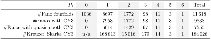
Table 6. The number of Fano fourfold hypersurfacesX withP1=h0(X,−KX)

and Calabi–Yau threefold hypersurfacesY with h0(Y,OY(1)) =P1−1.

P1 0 1 2 3 4 5 6 Total

#Fano fourfolds 1036 8697 1772 98 11 3 1 11 618

#Fanos with CY3 0 7953 1772 98 11 3 1 9838

#Fanos with quasismooth CY3 0 6014 1429 97 11 3 1 7555

#Kreuzer–Skarke CY3 n/a 168 813 15 016 179 14 3 1 184 026

is most striking for those 8697 Fano fourfolds with h0_(X,−K

X) = 1, since these have a unique

effective anticanonical divisor. In 6014 cases there is a corresponding quasismooth Calabi–Yau, and if Xis chosen generally in its family, then its anticanonical divisor is a quasismooth Calabi– Yau threefold. Some of the 8697 cannot have a quasismooth elephant because they possess a singularity not polarised with a one. For example, X16 ⊂ P(5,4,3,2,2,1) has a singularity

1

5(2,2,3,4); put another way, the degree one variable is the only possible tangent form at the

index five point. The elephant is still a Calabi–Yau threefold (for general such X), just not quasismooth.

There are also cases where the anticanonical divisor is never Calabi–Yau. For example,

X23⊂P(11,4,3,3,2,1) has anticanonical divisorS23⊂P(11,4,3,3,2). This has a hyperquotient

singularity of type ₁₁1(4,3,3,2; 1), in the notation of [19, (4.2)]. But any singularity of this type is not canonical: the given weighted blowup of the ambient space, of discrepancy only 1/11, extracts a divisor of discrepancy ≤ −1 from the threefold.

The FanoX43⊂P(21,14,6,1,1,1) is slightly different. Both this and any effective

anticanon-ical divisor must contain the plane P(21,14,6). For the fourfold, this is no problem; for its threefold elephant, this forces up the divisor class group, the price of which is a non-Q-factorial point, so certainly not quasismooth. This Fano fourfold is the ‘98th’ with P1 = 3 in the table

above, which does not match one of the 97 quasismooth Calabi–Yaus.

Tigers. Tigers were introduced by Keel–McKernan [13]. We follow Johnson–Koll´ar [11, Defi-nition 3.2]: on normal variety X, atiger is an effective Q-divisor D, numerically equivalent to −KX, for which the pair (X, D) is not Kawamata log terminal.

A sufficient condition under whichXddoes not admit a tiger is given in [11, Proposition 3.3]:

if Xd⊂P(a1, . . . , as) with a1 ≥a2 ≥ · · · ≥as thenX does not have a tiger ifd≤as−1as. This

condition never holds for hypersurfaces in the infinite series, but in the sporadic hypersurfaces in Theorem1.3(ii) there are 443 485 cases which satisfy this condition, and so for which no member has a tiger. Only one of these has terminal singularities, namely X112 ⊂P(28,24,21,16,13,11).

K¨ahler–Einstein metrics. Johnson–Koll´ar [11, Proposition 3.3] give conditions under which Xd

admits a K¨ahler–Einstein metric: ifXd⊂P(a1, . . . , as) witha1≥a2 ≥ · · · ≥as thenX admits

a K¨ahler–Einstein metric ifd < s−1

Of the sporadic hypersurfaces in Theorem1.3(ii) there are 490 083 cases for which every qua-sismooth member admits a K¨ahler–Einstein metric. Eight of these have terminal singularities:

X77⊂P(20,17,14,11,9,7), X80⊂P(20,16,15,13,10,7),

X80⊂P(20,16,15,13,9,8), X90⊂P(25,18,15,14,13,6), X90⊂P(30,18,13,12,11,7), X91⊂P(25,20,16,13,11,7),

X112⊂P(28,24,21,16,13,11), X120⊂P(40,24,21,15,11,10).

1.4. The Johnson–Koll´ar conjecture. Johnson and Koll´ar [11] relate three classes, which we describe below. In each case we define c:=b1+· · ·+bs−2.

(i) Well-formed weighted projective (s−3)-spacesP=P(b1, . . . , bs−2) which admit a

quasi-smooth memberT ∈ |−2KP|; in other words, thosePfor which there is a (not necessarily well-formed) quasismooth (s−4)-fold hypersurface

T2c ⊂P(b1, . . . , bs−2).

(ii) Well-formed quasismooth Calabi–Yau (s−3)-fold hypersurfaces

S2c⊂P(c, b1, . . . , bs−2).

(iii) One-parameter series of well-formed quasismooth hypersurfaces

X_d(k)(k) ⊂P(a

(k)

1 , . . . , a(k)s ) for oddk∈Z≥0,

whose weights are determined by the series

(a(k)₁ , a(k)₂ , . . . , a(k)_s , d(k)) = (c−1, b1, . . . , bs−2,2,2c) +k(c, b1, . . . , bs−2,0,2c).

It is clear that ifP(b1, . . . , bs−2) is well-formed in (i) then so are the correspondingSandX. That

quasismoothness passes from T to X is shown in [11, Lemma 2.4]. Indeed, given quasismooth

T: (f(z1, . . . , zs−2) = 0)⊂P, the hypersurface S: (y21 =f(y2, . . . , ys−1))⊂P(Pbi, b1, . . . , bs−2)

is quasismooth; conversely, given a quasismooth S, completing the square reveals a polynomial

f that defines a quasismooth T. Continuing with such anS, the hypersurface

X2kPbi:

x2₁xs=f(x2, . . . , xs−1) +xk

P

bi

s

⊂P−1 +kXbi, kb1, . . . , kbs−2,2

is quasismooth, and so the general hypersurfaceXis too. However, there is no clear reason why an arbitrary quasismooth series of X of that degree should arise from a quasismooth S.

Nevertheless, Johnson and Koll´ar conjecture that ifX_d(k)(k) ⊂P(a

(k) 1 , . . . , a

(k)

s ) is a one-parameter

series containing infinitely many well-formed, quasismooth hypersurfaces whose weights are de-termined by a series

(a(k)₁ , a(k)₂ , . . . , a(k)_s , d(k)) = (v1, . . . , vs+1) +k(w1, . . . , ws+1),

for fixed vectors v and w, then it is of type (iii) above, and furthermore it arises from a quasi-smooth T of type (i) lying in a well-formed weighted projective spaceP(b1, . . . , bs−2).

Well-formedness ofSin (ii) is not, by itself, sufficient to imply that the varieties in (i) and (iii) are well-formed. However, if S is well-formed then gcd{b1, . . . , bi−1, bi+1, . . . , bs−2}= 1 or 2 for

any i, hence the only way forP(b1, . . . , bs−2) to fail to be well-formed is by having an index two

stabiliser in codimension one. Exactly that failure is catastrophic for X, so we can rephrase the conjecture informally as: infinite series in dimension n with ωX = OX(−1) correspond to

hyperelliptic Calabi–Yau (n−1)-folds that do not have a locus of transverse 1₂(1,1) quotient singularities in codimension two that is fixed pointwise by the involution.

In dimension three there are 48 well-formed, quasismooth K3 surfaces of the form S2Pbi ⊂ P(Pbi, b1, b2, b3). Of these, 25 of the spacesP(b1, b2, b3) are well-formed, and these correspond

Corollary 1.4. The Johnson–Koll´ar conjecture holds when dimX= 4.

To check the corollary, it suffices to compare the list of 1597 series in Theorem 1.3 with the list of 7555 quasismooth Calabi–Yau threefold hypersurfaces. Within the latter, 2390 cases are double covers S₂Pbi ⊂ P(

P

bi, b1, b2, b3, b4). Of these, 1597 of the spaces P(b1, b2, b3, b4) are

well-formed. These correspond to the 1597 one-parameter series with d= 4,k=−1, exactly as predicted by the conjecture.

1.5. Orbifold rational curves and ADE singularities. To illustrate the basic method of classification, we will consider quasismooth projective curves

Cd: (Fd(x, y, z) = 0)⊂P(a, b, c) with d+ 1 =a+b+c.

Here we write F =Fd for a form of degree d. The numerical condition implies that gC = 0. To

carry out the analysis we enforce the order a≥b≥con the ambient weights.

Quasismoothness atPx= (1 : 0 : 0) implies that at least one ofxm,xm−1y, orxm−1z appears

(with non-zero coefficient) in F, for some m ≥ 2. In each case the monomial determines the degree d, and then the numerical condition implies thatm <3: indeed a≥b so 2a+c≥d+ 1, butd≥(m−1)a+c. We consider the three casesx2_{,xy, and xz∈F separately.}

If x2 ∈F then d= 2aand the condition reads a+ 1 =b+c. Quasismoothness at Py implies that at least one of ym−1_x,ym_{, ory}m−1_{z appears in F. The relation gives that 2b≥a+ 1, so}

that 3b+c ≥ d+ 2 and m ≤ 3. Thus the possible monomials at Py are y3, y2z, y2, and yz.

(Other cases are dismissed at once: xy2 implies d=a+ 2b≥a+b+c=d+ 1, whilst xy will be considered separately at Px.)

Again we consider the cases separately. If x2+y3 ∈F then we can assemble the numerical conditions together in a standard auxiliary matrix:

N =  

1 1 1 −1 1 2 0 0 −1 0 0 3 0 −1 0

 ,

where any positive integral element of the kernel ofN of the form (a, b, c, d,1) provides weights that satisfy the numerical conditions so far. We compute the kernel using the (integral) echelon form of N, which in this case is

 

1 0 3 −1 3 0 1 4 −1 4 0 0 6 −1 6

 .

This provides at once the solutions so far, namely a one-dimensional series

C6n: (x2+y3+· · ·= 0)⊂P(3n,2n, n+ 1), wheren≥1.

For small nwe understand these easily:

n Type Typical equation Numerics

1 D4 x2+y3+z3 C6 ⊂P(3,2,2)

2 E6 x2+y3+z4 C12⊂P(6,4,3)

3 E7 x2+y3+yz3 C18⊂P(9,6,4)

The case n= 4 is excluded since any curve C24 ⊂P(12,8,5) fails to be quasismooth at Pz. In

fact, this requirement at Pz implies that at least one of xzm−1, yzm−1, and zm appears in F,

which in turn implies that

m= ne

n+ 1, where e≤6, som <6 and this branch of the tree search is complete.

A similar exercise in the case when x2+y2z∈F leads to the echelon form 



1 1 0 −1 −1 0 2 0 −1 −2

0 0 1 0 2

 

which gives

C2n−2: (x2+y2z+zn−1 = 0)⊂P(n−1, n−2,2), where n≥4.

The equations in this case are the familiar Type Dn equations. All other branches of the tree

provide F with quadratic terms of rank at least two, and lead to Type An equations. Hence

we recover precisely the classification of ADE singularities as the affine cones on the resulting curvesC.

This simple exercise illustrates most of the ideas. In particular, even though we may have infinitely many solutions, the collections of all monomials that can give quasismoothness is finite and can be bounded at each step of the tree search. There is, however, an additional consideration: the hypersurfaces listed here are not well-formed. In the analysis below we enforce that additional condition too.

2. The quasismooth algorithm

We search for collections of integers

(a1, . . . , as, d) with a1 ≥ · · · ≥as ≥1

for which, for a general formFd of degreed, the hypersurface

Xd: (Fd(x1, . . . , xs) = 0)⊂Ps−1(a1, . . . , as)

is well-formed and quasismooth. We use this notation throughout, including the ordering on theai. We use Pi = (0 :· · ·: 1 : 0 :· · ·: 0), where the 1 is in theith position, to denote the ith

coordinate point of Ps−1_(a

1, . . . , as). (Note that the variables start with x1, not the usual x0,

and the ordering convention on the ai is the opposite of that in [11].)

We are mainly interested in those varieties whose singularities lie in some restricted class; see §3 for details. First, however, we make a complete list of the well-formed quasismooth hypersurfaces, irrespective of singularities. The conditions on the singularities are imposed afterwards. This is the same approach as taken in [10,11].

We learned the basic algorithm below from Miles Reid, who used it in [18] to compute the ‘famous 95’. The same approach is used by [10,11]: quasismoothness at 0-strata imposes a range of possible linear conditions on integral vectors (a1, . . . , as, d) that one must organise and solve.

2.1. Inequalities with semipositive and seminegative summation. Leta1 ≥a2 ≥ · · · ≥ as ≥ 1 be integers, and let p1, . . . , ps be any integers (here negative integers are allowed). We use the notation Σ+pℓ to denote the following number:

Σ+pℓ = s

X

ℓ=1 p′

ℓ,

where eitherp′

ℓ=pℓ≥0 or 0≥p′ℓ ≥pℓis chosen minimally so that each sump′ℓ+p′ℓ+1+· · ·+p′s≥

Equivalently, define the sequence σ0 := min{ps,0} and σi+1 := min{σi+ps−i−1,0}. Then

Σ+_p

ℓ = σs. We also define Σ−pℓ. Set τ0 := max{ps,0} and τi+1 := max{τi+ps−i−1}. Then

Σ−_{pℓ=τs. The following lemma is elementary.}

Lemma 2.1. In the notation above,

a1Σ+pi ≥a1p1+· · ·+asps

and

a1Σ−pi≤a1p1+· · ·+asps.

2.2. Quasismoothness at 0-strata. At each coordinate pointPi, quasismoothness requires a

monomial xm_i i−1xji ∈F for somemi ∈Z≥0 and some 1≤ji ≤n (the case ji =ioccurs when

Pi ∈/ X). These conditions do not necessarily restrict the search to a finite set of solutions – as

in [10] we expect some infinite series – but they do allow for a terminating search provided that we can handle certain infinite series. By recursively imposing these conditions at every point, we obtain a branching search-tree. The monomials appearing in F at each step are recorded in a matrix of exponents; this same matrix allows us to recognise when a branch of the tree has been exhausted.

We compare the degree of a Laurent monomialxn1

1 · · ·xnss, where each ni∈Z, with the degree

of F by recording the integers appearing in the expression

degx

n1

1 · · ·xnss Fm =e

as a row of integers

(n1, . . . , ns,−m, e).

We recursively build a matrix using these rows of integers, as explained below. We refer to this matrix as the tangent monomial matrix.

We always start in the same way by comparing the monomial x1· · ·xs, which has degree

a1+· · ·+as, withF itself; in this case the relative degree is minus the canonical degree kand

we record the first row of the tangent monomial matrix, which hass+ 2 columns, as

(1, . . . ,1,−1,−k).

Any polynomialF whose varietyX= (F = 0) is quasismooth atP1must include a monomial

of the formxm1

1 xj1 for some non-negative integerm1and for some variablexj1;j1 = 1 is allowed,

and thenP1∈/ X, which is fine. The crucial observation is that there are only finitely many pairs

(m1, j1) that can arise in this way. The number of pairs is bounded by the following lemma.

Lemma 2.2. Assume thats≥4.

(i) If k <0 then m1< s, and so the possible pairs (m1, j1) are

{(m, j)|m∈ {2,3, . . . , s−1}, j ∈ {1,2, . . . , s}}.

If 2−s < k <0 then the only case with m1= 2 that could arise is(2,1).

(ii) If k≥0 then m1≤s+k, and so the possible pairs (m1, j1) are

{(m, j)|m∈ {2,3, . . . , s+k}, j∈ {1,2, . . . , s}}.

Proof. The proof uses the numerics of adjunction: k=d−(a1+· · ·+as). IfX is quasismooth at P1 we need atangent monomial xm11−1xj ∈F, for some m1 ≥2 and j∈ {1,2, . . . , s}. Suppose

that k <0. Ifm1 ≥sthen

d= deg(xm1−1

1 xj) = (m1−1)a1+aj ≥

X

ai=d+ (−k)> d,

Suppose now that k≥0. Ifxm1−1

1 xj ∈F withm1≥s+k+ 1 then

d= (m1−1)a1+aj ≥

X

ai+ (m1−s)≥(d−k) + (k+ 1) =d+ 1,

which again is a contradiction. Hencem1 ≤s+k as required.

The additional restriction in (i) when −k < s−2 follows directly from adjunction, since

otherwise d−k=a1+aj−k <Pai.

For each pair (m1, j1) we use the row of exponents and degree to extend the matrix, so from

the first monomial we obtain the new tangent monomial matrix

1 1 · · · 1 1 1 · · · 1 −1 −k m1−1 0 · · · 0 1 0 · · · 0 −1 0

,

where the 1 in the second row is in the j1th position (we have illustrated the case whenj1 6= 1, but this is also a possibility). The integral echelon reduction of this matrix is

1 1 · · · 1 1 1 · · · 1 −1 −k

0 m1−1 · · · m1−1 m1−2 m1−1 · · · m1−1 2−m1 k(1−m1)

,

with a further simplification of the top row possible if m1= 2.

Set c = −(2−m1) ≥ 0 and b = k(1 −m1) – the final two entries of the last row, with

the indicated change of sign – and assemble all possible pairs (m2, j2) for which a monomial xm2−1

2 xj2 could exist to verify the quasismoothness of X at P2. The possible pairs (m2, j2) are

determined by considering the case when i= 2 in the following lemma.

Lemma 2.3. Suppose that when considering the ith 0-stratum Pi, the last row of the tangent monomial matrix in echelon form is

(

i−1

z }| {

0, . . . ,0, pi, pi+1, . . . , ps,−c, b),

where the first i−1 entries are zero, and pi >0.

(i) If c >0 then

mi≤ (

⌈(Σ+pℓ)/c⌉, if b≥0; ⌈(Σ+pℓ−b)/c⌉, otherwise.

(ii) If c <0 and all pℓ ≥0 then

mi≤ (

⌈(Σ−_{pℓ−b)/c⌉, if b≥0;} ⌈(Σ−_p

ℓ)/c⌉, otherwise.

(iii) If c= 0 and all pℓ ≥0 then there are no solutions if Ps_ℓ=ipℓ > b.

Proof. Recall the notation: aℓ = degxℓare the unknown positive integers that we are attempting to solve for, ordered in decreasing order. We seek possible (m, j) such that xm_i −1xj ∈ F; in particular, such monomials have the same degree as F. Given such a choice of (m, j), the current last row of the matrix

(0, . . .0, pi, pi+1, . . . , ps,−c, b)

implies that

deg x

pi

i · · ·x ps

s xm_i −1xj

c =b

hence aipi+· · ·+asps−cai(m−1)−caj =b.

(2.1)

Suppose first that c >0. By Lemma2.1,

Hence ai(Σ+pℓ−c(m−1))> b. Whenb≥0 we obtain (Σ+pℓ)/c > m−1, which gives the first

bound in (i). When b <0, dividing byai gives

Σ+pℓ−c(m−1)> b/ai ≥b,

which gives the second bound in (i).

Suppose now that c <0. The inequality (2.1) together with Lemma2.1implies that

aiΣ−pℓ+|c|ai(m−1) +|c|aj ≤b.

When b≥0 we obtain

Σ−pℓ+|c|(m−1)< b/ai ≤b,

giving the first bound in (ii). When b <0, usingb/ai ≤0 gives the second bound.

When c = 0 the same analysis does not give a relation between the degree of F and that of the monomial xpi

i · · ·x ps

s , so we do not get a bound on m. Nevertheless, if Ppℓ > b then

that monomial cannot have degree bfor any (positive integral) choice of weights; in this case we

conclude that there are no solutions, giving (iii).

Corollary 2.4. Suppose that c 6= 0 and i > 1. Let mmax be the upper bound for the mi in Lemma 2.3, determined according to the signs of b and c. Then the possible pairs (mi, ji) are

{(m, j)|m∈ {2,3, . . . , mmax}, j∈ {1,2, . . . , s}}.

Ifc6= 0 then Corollary2.4provides the possible choices for the next row of the tangent monomial matrix. We run through each of these in turn, repeating this step until either c= 0 ori=s−1. When either case occurs we move to the next step, described below, which is to use this system of equations encoded in the matrix to find all possible systems of weights.

2.3. Solving for possible weights. At this stage the tangent monomial matrix N is of size

r×s+ 2, for 2 ≤ r ≤ s. Note that it can happen that c = 0 and we stop growing N before it has s rows. Treating this as an auxiliary matrix, we solve the r inhomogeneous equations in s+ 1 unknowns (a1, . . . , as, d) – the inequalities a1 ≥ · · · ≥as ≥1 remain in force to avoid

repeating solutions and we solve for integral points of the resulting polyhedron. There is no reason why these solutions should represent well-formed and quasismooth hypersurfaces, so we perform some additional checks to eliminate infinite polyhedrons that could only contribute finitely many solutions.

The hyperbola trick. We repeatedly use the following “hyperbola trick”. Let a, b, c, d be fixed integers, and for simplicity suppose that d6= 0. Consider the expression

N = a+λb

c+λd.

What is the largest value of λ ∈Z for which N is an integer? Sketching the graph of N as a function of λanswers this at once. The geometry is controlled by the determinant

∆ = det

a b c d

.

2.4. One-parameter series of solutions. Consider the case when the solution polyhedron is one-dimensional, with integer points {u+λk|λ∈Z_≥0}, for some u = (u1, . . . , us+1), k =

(k1, . . . , ks+1)∈Zs+1, whereulies in the strictly positive quadrant. Consider a general solution

(u1+λk1, . . . , us+1+λks+1). We describe the tests we subject this series to in our implementation;

there is some overlap.

Quasismooth Test I: the final coordinate point. Suppose ks 6= 0, and consider the point Ps. If

xi is to be a tangent monomial at Ps (for any i, including the possibility that i = s when Ps

does not lie on the hypersurface) then xN

s xi ∈ F, for some N ∈ Z≥0. Computing degrees and

rearranging gives

(2.2) N = (us+1−ui) +λ(ks+1−ki)

us+λks .

We now apply the hyperbola trick described above. In this case N tends to (ks+1−ki)/ks as λ→ ∞, either from above or from below depending on the sign of the determinant

det

us+1−ui ks+1−ki us ks

.

In either case this gives a formula for the largest value of λ for which N in equation (2.2) is integral. If the determinant is zero then the hyperbola consists of two lines, one with λ = −us/ks<0 (which gives no solutions) and one with N = (ks+1−ki)/ks, which gives solutions

if and only if N is integral; in this case the series requires further analysis.

When the determinant is not zero, the maximum of these values for 1≤i≤sgives an upper bound of λ, and so this is not an infinite series of solutions after all: we compute the finitely many cases as sporadic solutions.

For example, consider the case u = (20,9,4,4,4,40) and k = (15,7,3,3,2,30). With this input, the determinant above is never zero, and this method detemines the maximum λ = 16. When interpreted as a weighted hypersurface, u+ 16k is indeed quasismooth; however, in this case it does not represent a well-formed hypersurface, so will be excluded at at later stage. The cases λ= 1, 3 and 13 all give rise to well-formed, quasismooth hypersurfaces:

X70⊂P(35,16,7,7,6), X130⊂P(65,30,13,13,10), X430 ⊂P(215,100,43,43,30).

Almost identical u,k. Ifuandkhaves−1 of the firstsentries in common, then no case beyond the first pointuis well-formed, so we may reject the rest of series and treatuas a sporadic case. If they have onlys−2 entries in common, andv=us+1−ks+1 6= 0, then the ambient space has a codimension two stratum with nontrivial stabiliser, so the equation must prevent that lying inside X. The only multiples ofλthat permit this are zero and the non-unit divisors ofv.

Complementary u, k modulo 2. A parity check on the sum of entries ofu and u+k also rules out the whole series in cases where the stabiliser Z/2 fixes a large coordinate subspace.

Quasismooth Test II: one-dimensional strata. If exactly onekℓ= 0 then we check for one-strata with equal ui and equalki where we can apply the hyperbola trick to boundλ.

Consider any one-stratum hxi1, xi2i withki1 =ki2 and ui1 =ui2. Suppose further that ks+1

is divisible by ki₁, but that us+1 is not divisible by ui₁. This implies that the one-stratum is contained in every hypersurface of the series. If this series really does contain infinitely many quasismooth members then there must be two tangent variables that work (numerically, at least) for infinitely manyλ.

SupposexN1

i1 x

N2

i2 xj ∈F. Calculating degrees and rearranging gives

N1+N2 =

(us+1−uj) +λ(ks+1−kj)

ui1 +λki1

The hyperbola trick applies. If for every j = 1, . . . , s, j 6=i1, i2, ℓ, the associated determinant

is non-zero then even requiring a single tangent variable along this one-stratum puts an upper bound onλ. (This one-stratum needs two tangent variables, which is why we do not impose the conditions on xℓ.) We can calculate this bound and regard all cases below it as sporadic cases.

Easy codimension two failure of well-formedness. Let (u1+λk1, . . . , us+1 +λks+1) be a

one-parameter series solution. Denote a general polynomial that defines the corresponding hyper-surface by Fλ.

Lemma 2.5. Suppose that there exists a subset I = {i1, . . . , ir} ⊂ {1, . . . , s−1} and α > 0 such that ui =αki for all i ∈I. Denote d=us+1 and e =ks+1. If for some λ >0 there is a monomial m=xp1

i1 · · ·x

pr

ir ∈Fλ for which p1ki1 +· · ·+prkir =e then (i) p1ui1+· · ·+pruir =d,

(ii) m∈Fλ for allλ≥0, and

(iii) d=αe.

Proof. Calculating the degree of the given monomial for the givenλ >0 gives

r

X

j=1

pj(uij +λkij) =d+λe

which, after rearrangement, gives

(2.3) λ

r

X

i=1

pjkij −e !

=d−

r

X

i=1 pjuij.

Part (i) follows immediately. Since this equation holds independently of λ, we obtain (ii). Finally, by substituting uij =αkij into (i) we obtain (iii).

The special caser =s−2 provides a well-formedness test, generalising the ‘almost identical’ test above. Suppose that u+λk is a one-parameter series as in Lemma 2.5 for which d6=αe. In this case, whenever λ > 0, the corresponding stratum PI has nontrivial stabiliser and so

cannot be contained in a well-formed hypersurface X. Therefore there must be a monomial

m∈Fλ, as in Lemma 2.5(ii). To avoid a contradiction, we must have that Ppiki−e6= 0. But

rearranging (2.3) for λgives

λ= d− P

piui

P

piki−e

= (d−αe) +αe− P

piαki

P

piki−e

= Pd−αe

piki−e

−α≤ |d−αe| −α.

This gives an upper bound onλ, so we may reject the one-parameter series and consider instead the finite number of solutions having these λas sporadic cases.

Quasismoothness at all proportional strata. The proof of Lemma 2.5also gives us a slight vari-ation.

Lemma 2.6. Suppose there exists a subset I ={i1, . . . , ir} ⊂ {1, . . . , s−1}and α >0such that ui = αki for all i∈ I. Set d:= us+1 and e := ks+1. If for some λ > 0 and h /∈ I there is a monomial m=xhxp1

i1 · · ·x

pr

ir ∈Fλ for which p1ki1 +· · ·+prkir =e−kh then (i) p1ui1+· · ·+pruir =d−uh, and

(ii) m∈Fλ for allλ≥0.

Suppose the stratum ΓI =P(ai1, . . . , air) is contained in the generalX. Any monomialm∈Fλ of the form in Lemma 2.6 gives a tangent variable along the stratum ΓI. To be quasismooth

along ΓI, there must exist at least r such monomials with distinct linear formsxh.

To use this as a test, we consider each h /∈ I in turn, positing a monomial m ∈ Fλ as in

tangent forms for every λ and we record this fact. Otherwise we may rearrange to obtain an upper bound for λwithxh a tangent form:

λ= d−uh− P

piui

P

piki+kh−e =

(d−uh+αkh−αe)−αkh+αe−αPpiαki

P

piki+kh−e

= dP−uh+αkh−αe

piki+kh−e

−α

≤ |(d−αe)−(uh−αkh)| −α

which again provides an upper bound for λ in terms of the series. If we find r independent tangent forms along ΓI then it can be contained inside a quasismooth X; if not, then these

bounds apply to limit the number of quasismooth members of the series.

2.5. Analysis of singularities. Since Xd⊂P(a1, . . . , as) is general, the quotient singularities

of the hypersurfaces can be described by following [9,§10]. We then apply the Reid–Shepherd-Barron–Tai criterion as given in [18, (3.1)] and [21, Theorem 3.3].

The orbifold strata on the ambient P(a1, . . . , as) correspond to subsets I ⊂ {1, . . . , s} of

indices for which rI := gcd{ai |i∈I}>1. We only need to work with maximalI for any given r = rI, and so we always assume this is the case. For example, any point on the relative big torus Π◦ _{⊂Π of the I ={4,5} stratum Π}

I ⊂P(1,3,5,8,12) has a quotient singularity of type 1

4(1,3,5) = 14(1,3,1) transverse to ΠI.

Given a hypersurfaceXd: (F = 0)⊂P(a1, . . . , as), consider an ambient orbifold stratum Π =

P(ai₁, . . . , ait) of transverse type

1

r(b1, . . . , bs−t). So {ai1, . . . , ait, b1, . . . , bs−t} = {a1, . . . , as}. One of two things can happen:

(i) F vanishes on Π, so that Π ⊂ X. In this case, at any point P ∈ X ∩Π◦_{, X has} a transverse quotient singularity of type 1_r(b1, . . . ,bbj, . . . , bs−t), where xj is a tangent

variable toX at P. Note that there may be several tangent variables at P, but their weights are congruent modulor and so any one may be used.

(ii) F = 0 cuts a codimension one locus transversely inside Π. In this case, at any pointP ∈

X∩Π◦_{, the hypersurfaceX has a transverse quotient singularity of type} 1

r(b1, . . . , bs−t).

This is enough to calculate the singularities of X.

Example 2.7. Consider X112 ⊂ P(28,24,21,16,13,11) in coordinates x, y, z, u, v, and w. The

ambient space has the following orbifold strata:

0-dimensional strata: ₂₈1(24,21,16,13,11), ₂₄1(4,21,16,13,11), ₂₁1 (7,3,16,13,11),

1

16(12,8,5,13,11), 131 (4,11,8,3,11), and 111 (6,2,10,5,2).

1-dimensional strata: Transverse 1₈(28,21,13,11) = 1₈(4,5,5,3) along the relatively open stratum inP(24,16); 1₇(3,2,6,4) alongP(28,21); and 1₃(1,1,1,2) alongP(24,21).

2-dimensional strata: Transverse 1₄(21,13,11) = ₄1(1,1,3) along P(28,24,16).

Since X is general it intersects the open two-stratum transversely in a curve of transverse

1

4(1,1,3) singularities. It also contains the P(24,21) stratum: the monomials y4u and z4x

provide tangent forms along it, so X has transverse type 1₃(1,1,2) in the open stratum. These two curves meet at the y-coordinate point P2, where y4u eliminates u, so is a dissident point

1

24(4,21,13,11). It does not pass through the 0-strata of indices 28 and 16, since there exist pure

power monomials x4 and u7. The remaining 0-strata do lie onX: the monomials z4x,v7z and

w8_{y (or w}9_{v) provide orbifold tangent equations at those points, which are therefore isolated}

terminal quotient singularities: ₂₁1(3,16,13,11), ₁₃1(2,11,3,11), and ₁₁1(6,10,5,2).

points each of type 1₈(4,5,5,3). Finally,X meets the open stratum ofP(28,21) in a single point of type 1₇(3,2,6,4) cut out by (x3_+z4_)x.

The monomials seen so far already describe terminal singularities, so define a Fano fourfold

X: (x4+y4u+z4x+u7+v7z+w8y= 0)⊂P(28,24,21,16,13,11).

3. Classifications of hypersurfaces

The main results of this paper concern fourfolds. Before discussing those, we recover known classifications in lower dimensions as a means of checking our implementation. There are also new results in these lower dimensions, but that is not what we focus on. The results in dimensions two, three, and four are summarised in Tables7,9, and11, respectively; details are available on the Graded Ring Database [3]. The varieties are polarised byA∈ |OX(1)|, and haveωX =OX(k)

for k = d−Pai. In particular, KX = kA and X is not embedded by ±KX unless k = ±1.

When k < 0 we say that X has index −k. We list only nondegenerate hypersurfaces, that is, those whose defining equation degree is not equal to one of the weights; degenerate hypersurfaces only arise in the anticanonical case when the index is bigger than the dimension.

3.1. Two-dimensional orbifold hypersurfaces. We summarise the results in Table7. The ‘famous 95’ weighted K3 hypersurfaces of Reid [18] is the first important result. The 62 cases of canonically polarised surfaces are not so familiar, but the four cases of these that are smooth are well known:

(3.1) X5⊂P3, X6⊂P(2,1,1,1), X8 ⊂P(4,1,1,1), and X10⊂P(5,2,1,1).

The anticanonically polarised surfaces are the result of Johnson–Koll´ar [10, Theorem 8]: the result is 22 sporadic cases and a single infinite one-parameter series. Higher index del Pezzo surfaces have been studied by Boyer, Galicki and Nakamaye [2], Cheltsov and Shramov [5], and Paemurru [16].

Table 7. Summary of results for surfaces, including the number of canonical, terminal, and smooth cases that occur among the series and sporadic results.

dim k #series #sporadic #can #term #sm Ref

2 −2 9 32† 4 1 1 [2,5,16]

2 −1 1 22 3 3 3 [10]

2 0 0 95 95 2 2 [18]

2 1 0 62 4 4 4

2 2 0 205 8 2 2

2 3 0 103 11 6 6

2 4 0 276 11 2 2

2 5 0 96 11 7 7

†_{A 33rd case X}

18 ⊂P(7,6,4,3) lies in a series but with the weights in a different order.

We consider the caseωX =OX(−2) in detail to illustrate the need for careful post-processing

but we do for Theorem 3.3below, which is sharp. Whilst the algorithm returns nine series and 37 sporadic cases, observation (with or without a computer) trims this to a sharp result of nine precisely-specified series and 32 sporadic cases.

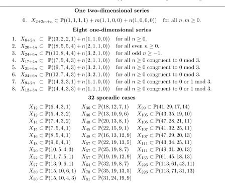
Theorem 3.1 (Index two del Pezzo hypersurfaces).

(i) The general member of each of the cases listed in Table 8 is a well-formed del Pezzo surface of index two with log terminal singularities.

(ii) Conversely, if Xd⊂P(a1, a2, a3, a4) is a well-formed del Pezzo surface of index two (so that a1+· · ·+a4 =d+ 2) with log terminal singularities then, possibly after reordering the ai, it is one of the cases listed in Table 8.

(iii) Of the surfaces in Table 8, only X2 ⊂ P3, X3 ⊂ P(2,1,1,1), X4 ⊂ P(2,2,1,1), and X6 ⊂P(3,2,2,1) have a member with canonical singularities, of which only the first has nonsingular member.

Table 8. All well-formed index two del Pezzo hypersurfaces with log terminal singularities.

One two-dimensional series

0. X2+2m+n⊂P((1,1,1,1) +m(1,1,0,0) +n(1,0,0,0)) for all n, m≥0.

Eight one-dimensional series

1. X6+2n ⊂ P((3,2,2,1) +n(1,1,0,0)) for all n≥0.

2. X20+4n ⊂ P((8,5,5,4) +n(2,1,1,0)) for all even n≥0.

3. X24+6n ⊂P((10,8,4,4) +n(3,2,1,0)) for all oddn≥ −1.

4. X17+4n ⊂ P((7,5,4,3) +n(2,1,1,0)) for all n≥0 congruent to 0 mod 3.

5. X21+6n ⊂ P((9,7,4,3) +n(3,2,1,0)) for all n≥0 congruent to 0 mod 3.

6. X24+6n ⊂P((12,7,4,3) +n(3,2,1,0)) for all n≥0 congruent to 0 mod 3.

7. X9+2n ⊂ P((4,3,3,1) +n(1,1,0,0)) for all n≥0 congruent to 0 or 1 mod 3.

8. X12+3n ⊂ P((4,4,3,3) +n(1,1,1,0)) for all n≥0 congruent to 0 or 1 mod 3.

32 sporadic cases

X12⊂P(6,4,3,1) X36⊂P(18,12,7,1) X99⊂P(41,29,17,14) X12⊂P(5,4,3,2) X36⊂P(13,10,9,6) X105⊂P(43,35,19,10)

X14⊂P(7,4,3,2) X40⊂P(20,13,8,1) X105⊂P(47,28,21,11) X15⊂P(7,5,4,1) X45⊂P(22,15,9,1) X107⊂P(41,32,25,11) X16⊂P(8,5,4,1) X48⊂P(16,13,12,9) X107⊂P(47,29,20,13) X18⊂P(9,6,4,1) X57⊂P(22,19,13,5) X111⊂P(43,34,25,11) X20⊂P(10,5,4,3) X57⊂P(25,19,8,7) X111⊂P(49,31,20,13) X22⊂P(11,7,5,1) X57⊂P(19,19,12,9) X135⊂P(61,45,18,13) X27⊂P(13,9,6,1) X64⊂P(32,19,8,7) X226⊂P(113,61,43,11) X30⊂P(15,10,6,1) X70⊂P(35,19,13,5) X226⊂P(113,71,31,13)

X30⊂P(15,10,4,3) X81⊂P(31,24,19,9)

Remark 3.2. The list of series and sporadic cases in Table 8 is given without repetition. The surfaceX18⊂P(7,6,3,4) is the initial casen=−1 in Series3. In that form, it does not respect

the ordering of weights that we imposed at the outset, but it falls naturally in the series and so we record it there. (Other works prefer to list this case separately, precisely because it breaks the ordering.) All other cases in the table have the conventional ordering.

(i) Series1 meets Series 0at X4 ⊂P(2,1,2,1) whenn=−1;

(ii) Series 2 meets Series 8at X12⊂P(4,3,3,4) whenn=−2;

(iii) Series3 meets Series 0at X6 ⊂P(1,2,1,4) whenn=−3;

(iv) Series 4 meets Series 0at X5 ⊂P(1,2,1,3) whenn=−3;

(v) Series6 meets Series 0at X6 ⊂P(3,1,1,3) whenn=−3; (vi) Series 7 meets Series 0at X5 ⊂P(2,1,3,1) whenn=−2;

(vii) Series8 meets Series 1at X6 ⊂P(2,2,1,3) whenn=−2.

Proof of Theorem 3.3. (i) and (iii) are routine: working in coordinates x, y, z, and t on wP3, we check that every hypersurface listed is well-formed and quasismooth, and identify those with canonical singularities.

Series 0 has a memberxy+z2+n+2m_+t2+n+2m_{= 0. This satisfies the conditions, which are}

open, and so the general member does too. This hypersurface meets potential orbifold strata in quotient singularities _1+n+m1 (1,1) and _1+m1 (1,1), which are canonical if and only ifn+m≤1.

We consider Series 8according to the residue of nmodulo 3. Ifn= 3k then

x2t+y2z+z2k+3+t9+2n= 0

meets the one-dimensional y-z orbifold stratum P(3(k+ 1),3) in two points and satisfies the conditions; it has a 1₃(1,1) singularity, which is not canonical. Ifn= 3k+ 1 then

x2t+y2z+xzk+2+t9+2n= 0

satisfies the conditions; again is not canonical. The remaining series and the sporadic cases are checked similarly.

(ii) follows from the correct implementation of the algorithm, followed by correct organisation of the output. The first step is to analyse the infinite series, confirming that each one does represent infinitely many quasismooth cases, and that the values of n in Table 8 are the only ones that work. For example, in Series 7, when n = 3k+ 2 the one-dimensional x-z orbifold stratum P(3(k+ 2),3) is contained in X, since 9 + 2n is not congruent to 0 modulo 3, so the hypersurface is not well-formed in this case. Other cases are treated similarly. The second step is then to exclude sporadic cases that lie in series, which is a routine observation.

3.2. Three-dimensional orbifold hypersurfaces. We summarise the results in Table 9. Some of these results are well known: the 7555 Calabi-Yau threefolds agree with Kreuzer– Skarke [15]; when k= 1 we recover Iano-Fletcher’s list [9] of 23 canonical hypersurfaces. The other classifications with k >0 are new, to the best of our knowledge. The classifications with

k <0 and terminal singularities agree with those obtained by Suzuki [4,20].

When k = −1 Johnson and Koll´ar [11, Theorem 2.2] classify all well-formed quasismooth threefold hypersurfaces with ωX = OX(−1). Our algorithm produces 4450 sporadic cases and

25 infinite series. Of these 4450 sporadic cases, eight lie in the infinite series (requiring the given order on theai). Removing these leaves 4442 sporadic cases and 25 infinite one-parameter series, in agreement with [11]. Note that [11] include a further 23 infinite series that satisfy all the conditions except for well-formedness, and that these series contain no well-formed cases. A further 14 sporadic cases lie in the series after relaxing the condition on the order of the ai. We choose not to remove them from the sporadic list; these cases are listed in Table 10. After checking the singularities, we recover the 95 cases of well-formed quasismooth terminal Fano threefolds discussed after Theorem (4.5) in [18], and in [11, Corollary 2.5].

We continue calculating in higher index. We say X is aFano threefold with canonical singu-larities if it satisfies the conditions for a Fano threefold with ‘terminal’ relaxed to ‘canonical’.

Table 9. Summary of results for threefolds, including the number of canonical, terminal, and smooth cases that occur among the series and sporadic results.

dim k #series #sporadic #can #term #sm Ref

3 −2 66 7084 96 8 3

3 −1 25 4442 95 95 2 [9,11,18]

3 0 0 7555 7555 4 4 [15]

3 1 0 6448 23 23 2 [9]

3 2 0 11 762 53 17 6

3 3 0 8298 76 27 2

3 4 0 13 305 110 25 7

3 5 0 7007 83 45 3

Table 10. Index one Fano threefolds that lie in infinite series after reordering their weights.

X6⊂P(2,2,1,1,1) X8 ⊂P(3,2,2,1,1) X10⊂P(4,3,2,1,1) X12⊂P(5,3,2,2,1) X12⊂P(5,4,2,1,1) X16⊂P(7,4,3,2,1) X16⊂P(7,5,2,2,1) X18⊂P(8,5,3,2,1) X20⊂P(9,5,4,2,1)

X22⊂P(10,7,3,2,1) X24⊂P(11,8,3,2,1) X26⊂P(12,7,5,2,1) X28⊂P(13,9,4,2,1) X36⊂P(17,12,5,2,1)

(i) There are66 one-parameter series and7084 sporadic cases of well-formed quasismooth threefold hypersurfaces with ωX =OX(−2).

(ii) There are 96 Fano threefold hypersurfaces of index two with canonical singularities. With the exception of the cubicX3⊂P4, they are all of the formXd⊂P(a1, a2, a3, a4,2), where Sd⊂P(a1, a2, a3, a4) is one of the 95 K3 hypersurfaces.

As in [20], three of these 96 hypersurfaces are nonsingular: X3 ⊂P4, X4 ⊂P(2,1,1,1,1,4),

and X6⊂P(3,2,1,1,1,6). A further five have terminal singularities:

X10⊂P(5,3,2,1,1), X18⊂P(9,5,3,2,1), X22⊂P(11,7,3,2,1),

X26⊂P(13,7,5,2,1) and X38⊂P(19,11,5,3,2).

We briefly describe the computer analysis. The raw output consists of 7102 sporadic cases and 85 series, 84 of which are one-dimensional, and one of which is two-dimensional. The two-dimensional series is

X3+2m+3n⊂P((1,1,1,1,1) +m(1,1,0,0,0) +n(1,1,1,0,0)).

When both m and n >0 this is not quasismooth along the one-stratum x1, x2: x3 is the only

tangent form there. This is really two one-parameter series

X3+2n⊂P((1,1,1,1,1) +n(1,1,0,0,0)) and X3+3n⊂P((1,1,1,1,1) +n(1,1,1,0,0)),

We can compute higher index, although proving precise statements about the infinite series becomes increasingly difficult as the number of results gets larger. We state the results which have canonical singularities, where the statements can be made precise.

Theorem 3.4 (Index three Fano hypersurfaces). There are 100 Fano threefold hypersurfaces of index three with canonical singularities. Of these 100 cases:

(i) 95 are of the formXd⊂P(a1, a2, a3, a4,3), where Sd⊂P(a1, a2, a3, a4) is one of the 95 K3 hypersurfaces, and so have a quasismooth K3 hypersurface elephant;

(ii) X2 ⊂P4, X3 ⊂P(2,1,1,1,1) and X4 ⊂P(2,2,1,1,1) have a quasismooth K3 elephant in codimension two;

(iii) X21⊂P(9,7,4,3,1) and X30⊂P(10,9,7,4,3) do not have a quasismooth K3 elephant.

As in [20], of these 100 hypersurfaces only the quadric is nonsingular, and a further six have terminal singularities: X3 ⊂P(2,1,1,1,1,3), X4 ⊂P(2,2,1,1,1,4), X6 ⊂P(3,2,2,1,1), X12 ⊂

P(5,4,3,2,1,12), X15⊂P(7,5,3,2,1), andX21 ⊂P(8,7,5,3,1).

Theorem 3.5 (Index four Fano hypersurfaces). There are 78 Fano threefold hypersurfaces of index four with canonical singularities. Of these 78 cases:

(i) 67 are of the formXd⊂P(a1, a2, a3, a4,4), where Sd⊂P(a1, a2, a3, a4) is one of the 95 K3 hypersurfaces, and so have a quasismooth K3 hypersurface elephant;

(ii) Six cases, X3 ⊂ P(2,2,1,1,1,3), X4 ⊂ P(2,2,2,1,1,4), X4 ⊂ P(3,2,1,1,1,4), X5 ⊂

P(3,2,2,1,1,5), X6 ⊂ P(3,3,2,1,1,6), and X6 ⊂ P(3,2,2,2,1,6) have a quasismooth K3 elephant in codimension two.

(iii) Five cases,X20⊂P(8,6,5,4,1,20), X28⊂P(10,8,7,4,3,28), X28⊂P(14,8,5,4,1,28), X36 ⊂P(18,8,7,4,3,36), and X44 ⊂ P(22,9,8,5,4,44) do not have a quasismooth K3 elephant.

Continuing in this fashion – listing Fano threefolds with canonical singularities of higher in-dex – there are 46 cases in inin-dex five, of which 43 have hypersurface K3 elephants, whilst

X4 ⊂ P(3,2,2,1,1), X6 ⊂ P(3,3,2,2,1), and X6 ⊂ P(4,3,2,1,1) have codimension two

ele-phants. There are 88 cases in index six, of which 69 have a hypersurface elephant, 17 have a codimension two elephant, and two cases – X24 ⊂ P(9,8,6,5,2) and X24 ⊂ P(11,9,8,6,5) – have no quasismooth K3 elephant.

3.3. Fano fourfolds. Our main results are the casesk=−1, 0, and 1. Whenk≥0 there are no infinite series and the raw output of the algorithm is ready to use.

We describe the case k = −1 in more detail in Steps 1–5 below. In this case raw output consists of four two-parameter series, 1611 one-parameter series, and 1 234 076 sporadic cases.

Step 1. The two-parameter series do not contain any good elements. The first case is the series corresponding to integral points in the polyhedron

(15,10,3,2,1,1,31) + cone{(15,10,3,2,0,0,30),(15,10,3,2,2,0,32)}.

The cone is not regular, but has three semigroup generators, including (15,10,3,2,1,0,31), so its integral points are all of the form

(15N,10N,3N,2N,1 +n2+ 2n3,1,30N + 1 +n2+ 2n3),

where N :=n1+n2+n3+ 1 and n1, n2, n3 ≥0. These integral points correspond to

X30N+1+n2+2n3 ⊂P(15N,10N,3N,2N,1 +n2+ 2n3,1).

Table 11. Summary of results for fourfolds, including the number of canonical, terminal, and smooth cases that occur among the series and sporadic results.

dim k #series #sporadic #can #term #sm

4 −2 4151† _{2 088 986}†† _{15 051 2304 2}

4 −1 1597 1 233 322 11 618 11 618 4

4 0 0 1 100 055 1 100 055 33 2

4 1 0 1 338 926 649 649 6

4 2 0 2 337 581 1373 504 2

4 3 0 1 318 278 1200 636 7

4 4 0 2 258 837 2079 596 3

4 5 0 1 291 194 1651 1017 5

†_{Experimental result based on 100 initial terms; series rejected by that test have not}

been proved to have no well-formed quasismooth members.

††_{Sporadic elements that lie in one of the series have not been removed from this list.}

The other three cases are

(4,3,3,2,1,1,13) + cone{(4,3,3,2,0,0,12),(4,3,3,2,2,0,14)},

(4,3,3,2,2,1,14) + cone{(4,3,3,2,0,0,12),(4,3,3,2,2,0,14)},

and (15,10,3,2,2,1,32) + cone{(15,10,3,2,0,0,30),(15,10,3,2,2,0,32)}.

They follow the same pattern as above; in each case the hypersurface corresponding to the vertex is already in the sporadic list.

Step 2. 1597 of the one-parameter families match those predicted by the Johnson–Koll´ar con-jecture, so they all work. We normalise them so they are the intersection of an affine line with the strict positive quadrant, irrespective of ordering of the vertex.

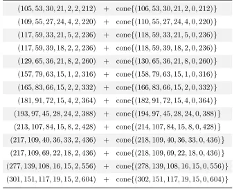
Step 3. The remaining 14 one-parameter series, listed in Table12, do not contain infinitely many good members. For example, consider the series

(213,107,84,15,8,2,428) + cone{(214,107,84,15,8,0,428)},

expressed as

X_428(n+1): (F = 0)⊂P(214(n+ 1)−1,107(n+ 1),84(n+ 1),15(n+ 1),8(n+ 1),2).

Thex3-x4 stratum Γ is contained in anyX(by mod 3 and mod 9 congruence). But we see that x1,x2, and x6 cannot be tangent forms along Γ unless n= 0. For example, if xa3xb4x6 ∈F then

84a+ 15b+ 2/(n+ 1) = 428, hence n = 0 or 1; and since b must be even, n 6= 1. Similarly

xa

3xb4x1 ∈/ F. Ifxa3xb4x2 ∈F then, again by computing degrees and dividing by 2(n+ 1), we have

that 28a+ 5b= 107, but this has no solutions with a, b∈Z_≥0. We conclude thatx5 is the only tangent form along Γ, and so X is not quasismooth unless n = 0. We add this initial n = 0 element to the sporadic list and exclude the series. The remaining cases work similarly: in each case we need to record the initial element but no others.

Table 12. Fourteen 1-parameter series excluded at Step 3.

(105,53,30,21,2,2,212) + cone{(106,53,30,21,2,0,212)}

(109,55,27,24,4,2,220) + cone{(110,55,27,24,4,0,220)}

(117,59,33,21,5,2,236) + cone{(118,59,33,21,5,0,236)}

(117,59,39,18,2,2,236) + cone{(118,59,39,18,2,0,236)}

(129,65,36,21,8,2,260) + cone{(130,65,36,21,8,0,260)}

(157,79,63,15,1,2,316) + cone{(158,79,63,15,1,0,316)}

(165,83,66,15,2,2,332) + cone{(166,83,66,15,2,0,332)}

(181,91,72,15,4,2,364) + cone{(182,91,72,15,4,0,364)}

(193,97,45,28,24,2,388) + cone{(194,97,45,28,24,0,388)}

(213,107,84,15,8,2,428) + cone{(214,107,84,15,8,0,428)}

(217,109,40,36,33,2,436) + cone{(218,109,40,36,33,0,436)}

(217,109,69,22,18,2,436) + cone{(218,109,69,22,18,0,436)}

(277,139,108,16,15,2,556) + cone{(278,139,108,16,15,0,556)}

(301,151,117,19,15,2,604) + cone{(302,151,117,19,15,0,604)}

Step 4. Remove any members of the sporadic list that lie in the series. The form of the Johnson– Koll´ar conjecture helps: rather than testing membership, one can simple observe when a sporadic case is of the right form; this also finds sporadic elements who lie in a series after re-ordering. There are 768 sporadic elements that lie in the series, of which 381 only do so after re-ordering; we remove these cases from the sporadic list.

Step 5. Check for canonical singularities in the sporadic list and the series. Again, the form of the Johnson–Koll´ar conjecture helps: every member of a series has the form

X_2hPbi ⊂P(−1 +h X

bi, hb1, . . . , hbs−2,2),

wheren≥3 andh≥1 is odd. Whenever h >1, the (s−3)-stratum P(hb1, . . . , hbs−2) has

non-trivial stabiliser Z/h, and X intersects this in codimension two on X. Its transverse quotient type is 1_h(h−1,2), which is not canonical when h ≥3 and so, in particular, X does not have canonical singularities when h >1. Hence we need only check the sporadic cases and the first member of each series.

3.4. Higher index Fano fourfolds: experimental results. There is no known sharp upper bound for the index of Fano fourfold hypersurfaces. For Fano threefolds, Suzuki [20, Theorem 0.3] proves that the highest Fano index is realised by a weighted projective space, and Prokhorov [17, Theorem 1.4] proves that only weighted projective space achieves this. Taking this as a guide, one may expect the highest index of a (Q-factorial terminal) Fano weighted projective space to be an upper bound. The classification of all such P(a1, . . . , a5) is known [12, Theorem 3.5]:

there are 28 686 cases in total, and the highest index is 881, realised by P(430,287,123,21,20). Although we have the raw results in a few higher indices, we only discuss the case of index two here, where we give an experimental overview, as we explain below. The raw output in this case consists of 5799 series and of 2 088 986 sporadic cases.

typically every other element represents a well-formed quasismooth hypersurface. This has given us computer-assisted rigorous proofs. We now adopt a more experimental approach: in what follows we reject any series that does not have a well-formed quasismooth element in its first 100 terms (in practice we have experimented with increasing the number of terms considered, and have found no difference in outcome).

There are five two-dimensional series, but these do not contribute anything other than existing dimensional series or sporadic results, so we reject them. Among the remaining 5794 one-dimensional series, 1643 have no good cases among the first 100 elements, and so we reject these too. This leaves 4151 one-dimensional series. These fall into several different types. The largest is a natural generalisation of the Johnson–Koll´ar series, but with a6 = 4:

X_d(k) ⊂P(a(k)₁ , . . . , a(k)₆ ) for evenk≥0, where

(a(k)₁ , . . . , a(k)₆ , d(k)) =Xbi−2, b1, . . . , b4,4,2

X

bi+kXbi, b1, . . . , b4,0,2

X

bi

for each of the 2390 well-formed quasismooth Calabi–Yau threefoldsS₂P_bi ⊂P(Pbi, b1, . . . , b4).

Note that, in contrast to the Johnson–Koll´ar correspondence in index one, we do not restrict to those 1597 cases with well-formed P(b1, . . . , b4).

Another large type is similar: there are 1585 cases with a6 = 3 of the form

(a(k)₁ , . . . , a(k)₆ , d(k)) =b1−1, b2, b3, b4, b5,3,

X

bi

+kb1, b2, b3, b4, b5,0,

X

bi

where XPbi ⊂ P(b1, b2, b3, b4, b5) is a Calabi–Yau threefold hypersurface that is a triple cover P

bi = 3b1 (in some cases after reordering so thatb1 is no longer the biggest of thebi), andk is

constrained modulo 3.

The remaining cases also form patterns:

3 cases: (a5 =a6= 1) For all k≥0

(a(k)₁ , . . . , a(k)₆ , d(k)) =b1, b2, b3,1,1,1,

X

bi+ 1

+kb1, b2, b3,0,0,0,

X

bi

where (b1, b2, b3) = (1,1,1), (2,1,1) or (3,2,1). 95 cases: (a5 =a6 = 1) For allk≥0

(a(k)₁ , . . . , a(k)₆ , d(k)) =b1, b2, b3, b4,1,1,

X

bi+kb1, b2, b3, b4,0,0,

X

bi

whereXPbi ⊂P(b1, b2, b3, b4) is any of the 95 K3 hypersurfaces.

48 cases: (a5 = 2, a6 = 1) For allk≥0

(a(k)₁ , . . . , a(k)₆ , d(k)) =b1−1, b2, b3, b4,2,1,

X

bi

+kb1, b2, b3, b4,0,0,

X

bi

whereXPbi ⊂P(b1, b2, b3, b4) is any of the 48 K3 hypersurfaces that are double covers. A further8 casesarise from these K3 surfaces, also witha5= 2,a6 = 1, but with more adjustments to the first three entriesb1, b2, b3 of the initial term.

22 cases: (a6 = 3) For k subject to a condition modulo 3, with kernels similarly

deter-mined by certain Calabi–Yau threefolds, but where the weights of the initial term of the series is half the kernel after two entries are slightly modified. For example:

(15,6,5,3,3,3,33) +k(33,11,10,6,6,0,66) fork≡2 mod 3,

and (9,5,4,1,1,3,63) +k(21,10,7,2,2,0,42) fork≡1 or 2 mod 3.

We do not see a single systematic pattern to this classification of infinite series, but it does still seem to be determined by Calabi–Yau hypersurfaces of lower dimension.

3.5. Higher dimensions.

Nonsingular weighted hypersurfaces. If Xd⊂P(a1, . . . , as) is nonsingular then

Y_d(n) ⊂P(a1, . . . , as, n

z }| { 1, . . . ,1)

is a nonsingular (n+s−2)-fold for any n ≥ 0. The converse holds too: smoothness for any

n ≥ 0 implies smoothness for them all. Whilst it is easy to make nonsingular hypersurfaces of general type with empty canonical system – for example, X30 ⊂P(5,3,2) – that necessarily

involves high degree equations, d=a1· · ·as at least. So it is not a surprise that the numbers

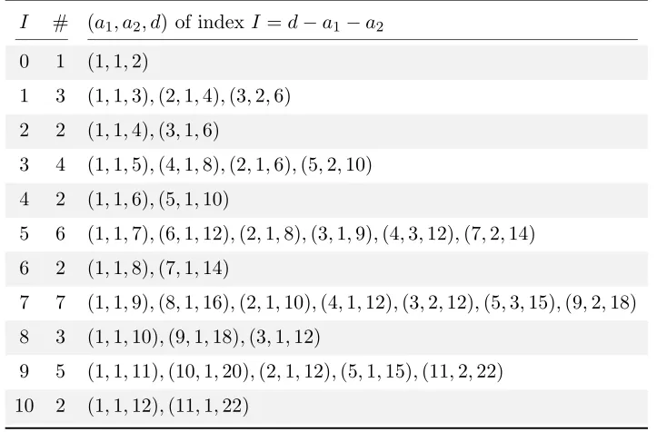
of smooth cases in dimensions three and four in Tables 9and 11 match exactly the numbers of smooth surfaces in Table 7. We list the first cases in Table 13, presented as (not necessarily well-formed) orbifold zero-dimensional schemes Zd⊂P(a1, a2).

Table 13. The orbifold zero-dimensional schemesZd⊂P(a1, a2) of index I ≤10

I # (a1, a2, d) of index I =d−a1−a2

0 1 (1,1,2)

1 3 (1,1,3),(2,1,4),(3,2,6)

2 2 (1,1,4),(3,1,6)

3 4 (1,1,5),(4,1,8),(2,1,6),(5,2,10)

4 2 (1,1,6),(5,1,10)

5 6 (1,1,7),(6,1,12),(2,1,8),(3,1,9),(4,3,12),(7,2,14)

6 2 (1,1,8),(7,1,14)

7 7 (1,1,9),(8,1,16),(2,1,10),(4,1,12),(3,2,12),(5,3,15),(9,2,18)

8 3 (1,1,10),(9,1,18),(3,1,12)

9 5 (1,1,11),(10,1,20),(2,1,12),(5,1,15),(11,2,22)

10 2 (1,1,12),(11,1,22)

Series of Fano five-folds. Fano five-folds that have quasismooth Calabi–Yau fourfold elephants arise directly from the 1 100 055 hypersurfaces: simply include an additional one amongst the weights. But we can also use Calabi–Yau fourfolds to describe infinite series of anticanonically-polarised five-fold hypersurfaces using Johnson and Koll´ar’s construction: 360 346 of the Calabi– Yau hypersurfaces are double covers V₂Pbi ⊂ P(

P

bi, b1, . . . , b5), and of these 261 195 have

P(b1, . . . , b5) well-formed. Each of these determine an infinite series according to the Johnson–

Koll´ar recipe of §1.4. In each series, only the initial element could possibly have terminal singularities, and 31 400 Fano five-folds of the form X₂Pbi ⊂ P(−1 +

P

bi, b1, . . . , b5,2) arise

in this way. In fact 25 276 of these 31 400 cases already arise in the usual way by including an additional one among the weights of a Calabi–Yau fourfold: cases like X10⊂P(4,1,1,1,1,1,2)

can be realised by both approaches.

3.6. Notes on computation and raw results. Our implementation of the algorithm can be downloaded from [3]. The results can be downloaded as plain-text files, or may be queried online. The code was run on version 2.21-1 of the Magma computer algebra system [1].

Table 14. Raw data from the algorithm in dimension 2.

k −5 −4 −3 −2 −1 0 1 2 3 4 5

#series 14 17 6 9 1 0 0 0 0 0 0

#sporadic 11 21 14 37 22 95 62 205 103 276 96

Runtime (s) 2 3 2 2 1 0.5 1 3 4 8 10

Table 15. Raw data from the algorithm in dimension 3.

k −5 −4 −3 −2 −1 0 1 2 3 4 5

#series 90 133 59 85 25 0 0 0 0 0 0

#sporadic 3178 6065 4354 7102 4450 7555 6448 11762 8298 13305 7007

Runtime (s) 289 347 176 149 72 59 171 392 649 1154 1225

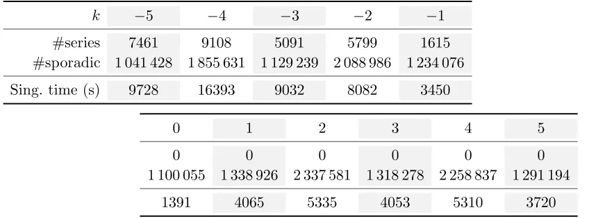
Table 16. Raw data from the algorithm in dimension 4.

k −5 −4 −3 −2 −1

#series 7461 9108 5091 5799 1615

#sporadic 1 041 428 1 855 631 1 129 239 2 088 986 1 234 076

Sing. time (s) 9728 16393 9032 8082 3450

0 1 2 3 4 5

0 0 0 0 0 0

1 100 055 1 338 926 2 337 581 1 318 278 2 258 837 1 291 194

1391 4065 5335 4053 5310 3720

with the size of the raw output. In dimension four the search tree is too large to be tackled reasonably in a single run. Instead, we run the algorithm to recursive depth one and compute the possible monomials at the first coordinate pointP1. We then run each of these as a single process

on a high-performance computing cluster of about 200 cores, together with a data management layer to handle results, failed processes, and so on. This runs in the order of an hour. Text files containing the results, and functions to parse them as Magma input, are available at [3]. We record the numbers of raw output and the timings to compute singularities in Table 16.

Acknowledgments. We are grateful to Miles Reid and Olof Sisask who explained this algo-rithm to us in the first place, and whose re-implementation of it in 2005 to recalculate the 7555 Calabi–Yau threefolds for the database at [3] was our starting point, and also to Jennifer Johnson and J´anos Koll´ar for discussion of their conjecture. Our thanks to John Cannon for providing Magma for use on the Imperial College mathematics cluster and to Andy Thomas for technical support. This work was supported in part by EPSRC grant EP/E000258/1. AK is supported by EPSRC grant EP/I008128/1 and ERC Starting Investigator Grant number 240123.

References

[1] Wieb Bosma, John Cannon, and Catherine Playoust. The Magma algebra system. I. The user language.J. Symbolic Comput., 24(3-4):235–265, 1997. Computational algebra and number theory (London, 1993). [2] Charles P. Boyer, Krzysztof Galicki, and Michael Nakamaye. Sasakian geometry, homotopy spheres and