Accepted Manuscript
Automatically deriving cost models for structured parallel processes using hylomorphisms
David Castro, Kevin Hammond, Susmit Sarkar, Yasir Alguwaifli
PII: S0167-739X(17)30728-8
DOI: http://dx.doi.org/10.1016/j.future.2017.04.035 Reference: FUTURE 3437
To appear in: Future Generation Computer Systems
Received date : 24 March 2017 Accepted date : 21 April 2017
Please cite this article as: D. Castro, et al., Automatically deriving cost models for structured parallel processes using hylomorphisms,Future Generation Computer Systems(2017), http://dx.doi.org/10.1016/j.future.2017.04.035
An operational semantics of a queue language for streaming
computations.
An operational semantics of algorithmic skeletons using this queue
language.
Derive cost equations for algorithmic skeletons from the operational
semantics.
Automatically Deriving Cost Models for Structured
Parallel Processes Using Hylomorphisms
David Castro, Kevin Hammond, Susmit Sarkar, Yasir Alguwaifli
School of Computer Science, University of St Andrews, St Andrews, UK.
Abstract
Structured parallelism using nested algorithmic skeletons can greatly ease the task of writing parallel software, since common, but hard-to-debug, problems such as race conditions are eliminated by design. However, choosing the best combination of algorithmic skeletons to yield good parallel speedups for a spe-cific program on a spespe-cific parallel architecture is still a difficult problem. This paper uses the unifying notion ofhylomorphisms, a general recursion pattern, to make it possible to reason about both the functional correctness properties and the extra-functional timing properties of structured parallel programs. We have previously used hylomorphisms to provide a denotational semantics for skele-tons, and proved that a given parallel structure for a program satisfies functional correctness. This paper expands on this theme, providing a simple operational semantics for algorithmic skeletons and a cost semantics that can be automat-ically derived from that operational semantics. We prove that both semantics are sound with respect to our previously defined denotational semantics. This means that we can now automatically and statically choose a provably optimal parallel structure for a given program with respect to a cost model for a (class of) parallel architecture. By deriving anautomatic amortised analysis from our cost model, we can also accurately predict parallel runtimes and speedups.
1. Introduction
In previous work [9], we have defined a type-based mechanism for reasoning about the safe introduction of parallelism using a structured parallel approach. Our approach allows us to extract parallel program structure as a type. Given a suitable model of a program’s execution cost (e.g. in terms of its time perfor-mance), we can reason formally about performance improvements for alterna-tive parallelisations, and so select aprovably optimal parallel implementation. In this paper, we show how to derive appropriate cost models formally from the
Email addresses: [email protected](David Castro),[email protected]
(Kevin Hammond),[email protected](Susmit Sarkar),[email protected](Yasir Alguwaifli)
*Manuscript with source files (Word document)
fkg Op. Sem.
dequeue(q1) eval(g)
dequeue(q2) enqueue(q3) eval(f)
enqueue(q4) . . .
Cost Trace
Tdequeue(q1) Tg
Tdequeue(q2) Tenqueue(q2) Tf
Tenqueue(q3) . . .
Derive Eqn. max
Tf,
Tg
[image:4.595.128.480.108.239.2]
+hoverheadi
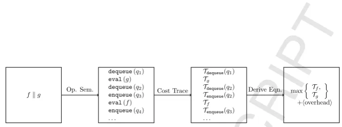
Figure 1: Deriving Cost Equations from Operational Semantics.
parallel structure of a program, using a new queue-based operational semantics. This gives a completely formal system for reasoning about the performance of structured parallel programs. We combine related work onalgorithmic skeletons
andrecursion schemes. Algorithmic skeletons [11] are parametric implementa-tions of common patterns of parallel programming. Using a pattern/skeleton approach, the programmer can design and implement a parallel program in a top-down manner. For example, the programmer could first identify the parallel patterns that occur in a particular piece of software, then select the patterns that potentially lead to the best speedups, and finally select a suitable implementa-tion for those patterns, as a composiimplementa-tion of one or more algorithmic skeletons. This composition then exposes theparallel structureof the implementation. De-veloping an equational theory for easily, and automatically, changing the parallel structure of a program has been the subject of research in the skeletons com-munity for the last two decades [42, 3, 1, 8]. Over a similar timeframe, in the functional programming community, a structured form of recursion has been explored, in the form ofpatterns of recursion, orrecursion schemes [31]. Re-search on this topic has brought many improvements to equational reasoning in functional languages. One example is the application of the laws and properties of recursion schemes to the well-knowndeforestation optimisation [47, 36].
1.1. Novel Contributions
In this paper, we show how to formally derive appropriate cost models from the parallel structure of a program, using a new queue-based operational semantics. This gives a completely formal system for reasoning about the performance of structured parallel programs. The main novel contributions of the paper are:
• We define the operational semantics of aqueue language that is powerful enough to describe the operational semantics of a number of algorithmic skeletons, and small and restrictive enough to facilitate reasoning about correctness and execution times (Sec. 4).
• We define theoperational semantics of a number of key algorithmic skele-tons using this queue language (Sec. 5).
• We derive a set of cost equations for a number of algorithmic skeletons from the operational semantics in a systematic way. We combine these cost equations with the notion ofsized types, and sketch how this process can be automated (Sec. 6).
1.2. Motivating Example
We illustrate our approach using theimage merge example from [9]. The pur-pose of theimgMergefunction is tomarkand thenmergepairs of images.
imgMerge : List(Img×Img) → ListImg imgMerge = map (merge ◦ mark)
This has many possible, semantically equivalent, parallel implementations.
imgMerge1 = farmn (fun(merge◦mark))
imgMerge2 = farmm (funmark)kfarmn (funmerge)
imgMerge3 = farmn (funmark)kfunmerge . . .
Here, farm n is a task farm skeleton that replicates its argument n times, fun
captures primitive (sequential) functions,◦is the normal function composition, andk is a parallel pipeline, i.e. the parallel composition of two skeletons. The structure of each parallel implementation can be lifted into an appropriate type signature, so that
imgMerge1 : List(Img×Img)
farmn(fun(merge◦mark))
−−−−−−−−−−−−−−−−−→ ListImg
2. Algorithmic Skeletons
We use algorithmic skeletons [11] to represent structured parallel patterns. Skeletons are parameterised templates (higher-order functions) that capture the structure of a parallel program. That is, they implement a specific parallel
pattern, that can be instantiated to produce a specific parallel algorithm. In this paper, as in our earlier work [9, 21], we use a “pluggable” approach, where all skeletons arestreaming entities (that is, they operate over multiple inputs and produce multiple results). Each skeleton takes its inputs from an input queue, and produces aresult queue. This approach allows skeletons to be easily nested or linked together into more complex structures, whose sub-components are connected via intermediate queues. In this paper, we will consider four common parallel skeletons,task farms, parallel pipelines, feedbacks, andparallel divide-and-conquer, plus one basic building block, structured functions.
. . . ,x6, x5 f f x2, f x1, . . .
x3 x4
Structured Functions(funf)lift basic (sequentially executed) functions so that they can be used as building blocks for our skeletons. These may be either named functions; compositions of one or more structured functions, constructed using thesequential composition operator (◦); or recursive functions that have been built using common patterns of recursion. Structured functions expose the underlying structure of a computation, enabling possible parallelisations.
. . . ,x12,x11,x10
f f f
f x2,f x1,f x3, . . . x7
x9
x8
f x5 f x6
f x4
Task farms(farm) apply the same operation to each element of an input stream of tasks, using a fixed number of parallel workers. The input tasks must be in-dependent, and the outputs can be produced in an arbitrary order.
. . . ,x12,x11,x10 x9 f f x8 f x7,f x6,f x5
f x4 g g(f x3)
g(f x2),g(f x1), . . .
. . . ,x9, x7, f x2 f f (f x1), f x3, . . .
x6 f x5
f x4
Feedbacks(fb) capture recursion in a streaming computation, operating over some internally nested skeleton with a given predicate e.g. f. This could be used, for example, to repeatedly transform an image using some parallel skele-ton until a certain dynamic condition was met.
div x
div div
x1 xn
div · · · div · · · div · · · div
x11 x1n xn1 xnn
conq · · · conq · · · conq · · · conq
· · · ·
conq conq
y11 y1n yn1 ynn
conq
y1 yn
y
Parallel Divide-and-Conquers(dc) are parallel implementations of classical divide-and-conquer algorithms. Parallelism comes from performing each of the recursive calls in the divide-and-conquer in parallel. In our framework, each instance of a divide-and-conquer skeleton divides an input into n sub-inputs using an+ 1-ary operation, so that we do not need to assume associativity.
3. A Type-Level Treatment of Parallel Structure
3.1. Functors
We begin by defining some basic concepts from category theory. Afunctor is a structure-preserving mapping betweencategories. We will only require end-ofunctors onCPO, F : CPO →CPO, which will represent type constructors,
Bifunctors are defined using products and sums alone. Functors are defined using apointed notation, with the obvious semantic interpretation. IfAandB
are type variables, andT is a type, we accept the following definitions:
G A B = T (bifunctor defined using sums and products)
F A = T (functor defined using sums and products)
F A = G T A (Gis a bifunctor)
F A = µ(G A) (Gis a bifunctor)
Example 1(Lists). Given the bifunctor L A B= 1 +A×B, the polymorphic
Listdata type is defined by the fixpoint of L A: ListA=µ(L A).Note that given a base bifunctor G A B , the data type F A=µ(G A) is also a functor. The two list constructors are defined in a standard way:
nil : ListA
nil = inL A (inj1 ())
cons : A→ListA→ListA
cons x l = inL A (inj2 (x,l))
3.2. Hylomorphisms
Hylomorphisms are a well known, very general, recursion pattern [31], that can be seen as a generalised divide-and-conquer pattern. Intuitively, hyloF f g is a regular recursive algorithm (i.e. with no nested or mutual recursion), where
g describes how the algorithm divides the input problem into sub-problems, stored in a structureF, andf describes how these results are combined.
hyloF : (F B→B)→(A→F A)→A→B
hyloF f g = f ◦F (hyloF f g)◦g
Catamorphisms(folds),anamorphisms(unfolds) andmapsare just special cases of hylomorphisms.
T A = µ(F A)
mapT f = hyloF A (inF B◦(F f id))outF A, whereA=dom(f) andB =codom(f)
cataF f = hyloF f outF
anaF f = hyloF inF f
For any recursive type that is defined as the fixpoint of a functor, µF, the standard inF : FµF → µF and outF : µF → FµF capture the isomor-phism betweenFµF and µF. Note that, since outF ◦inF =id, hyloF f g =
cataF f ◦ anaF g.
Example 2 (Quicksort). Assuming a type A, and two functions, leq and gt
that filter the elements appropriately, we can implement na¨ıve quicksort as:
qsort : ListA→ListA
qsort nil = []
We make the recursive structure explicit by using a tree. The split function unfolds the arguments into this tree, and thejoin function then flattens it.
split : ListA→Tree A
split nil = empty
split (cons x l) = node(split (leqx l))x (split(gtx l))
join : TreeA→ListA
join empty = nil
join (node l x r) = joinl++ consx (join r)
qsort : ListA→ListA
qsort = join◦split
We can remove the explicit recursion from these definitions, since split is a tree anamorphism, andjoin is a tree catamorphism.
split : ListA→T A (ListA)
split nil = inj1 ()
split (consx l) = inj2 (x, leqx l, gtx l)
join : T A(ListA)→List A
join (inj1 ()) = nil
join (inj2 (x,l,r)) = l++cons x r
qsort : ListA→List A
qsort = cataT A join◦anaT A split
Finally, since we have a composition of a catamorphism and an anamorphism, we can writeqsort as the equivalent hylomorphism.
qsort=hyloT A join split
3.3. Type System and Semantics
The syntax of expressions,E, is shown below. We distinguish between two levels of expressions: Structured Expressions (S)describe primitive (sequential) forms, andStructured Parallel Processes (P)introduce specific parallel skeletons.
e∈E ::= s | parT p
s∈S ::= f | e1 ◦ e2 | hyloF e1e2
p∈P ::= funs |p1kp2 |dcn,F s1 s2 |farmn p |fb p
3.3.1. Denotational Semantics
Our denotational semantics is likewise split into two parts: SJ·K describes the base semantics, andJ·Klifts this to astreaming form. We use a global environ-ment for atomic function types,ρ, and the corresponding global environment of functions, ˆρ:
SJp : T A→T BK : [[A→B]] SJfunfK = ρˆ(f)
SJp1 k p2K = SJp2K◦ SJp1K SJfarmn pK = SJpK
SJfbpK = iter SJpK
SJdcn,T,F f gK = cataF (ˆρ(f))◦anaF (ˆρ(g))
Jp : T A→T BK : [[T A→T B]]
JpK = mapT SJpK
Here◦denotes the usual function composition;iter captures the iterative struc-ture of a feedback skeleton (the usualtrampolinefunction [9]); andcataandana
are the usual cata/anamorphisms. Instead of assuming a dynamic termination condition, we require the worker operation,p, of a feedback loop,fbpto return a sum typeA+B. The feedback skeleton will applyp to a stream of inputs of typeA, merging any results of typeAwith the other inputs, and returning any results of typeB as its outputs. Since theiter,cata, ana andmap operations are all instances ofhylomorphisms, it follows that there is a single, underpinning theoretical formulation for all our skeleton forms, and it also follows that our structured programs may be easily transformed to introduce/remove parallelism in a provably sound way. We will achieve this using a type system.
3.3.2. The Structure-Annotated Type System
We annotate top-level program types with an abstraction of theparallel structure
of the program,σ ∈ Σ. Figure 2 shows our structure-annotated type system. Intuitively, Σ is a “pruned” version of E that retains information about how
the computation is performed, while removing as many details as possible about
what is being computed. We once again split its definition into two levels, Σs for sequential structures, and Σp for parallel ones.
σ ∈Σ ::= σs |parF σp
σs∈Σs ::= a|σ◦σ| hyloF σ σ
σp∈Σp ::= funσs | dcn,F σs σs
| σpkσp | farmn σp | fbσp
3.3.3. Convertibility
Our type system needs to include a non-structural rule that captures the con-vertibility relation,≡, for Σ.
`e : A−→σ1 B σ1≡σ2 `e : A7−→σ2 B
ρ(f) =A→B
`f : A−→a B
`e1 : B−→σ1 C
`e2 : A σ2
−→B
`e1◦e2 : A σ1◦σ2
−−−−→C
`e1 : F B −→σ1 B
`e2 : A σ2
−→F A G = baseF
`hyloF e1 e2 : A
hyloGσ1σ2
−−−−−−−−−→B
`p : T A−→σ T B F = baseT
`parT p : T A
parF σ
−−−−−→T B
` s : A−→σ B
` funs : T A−−−−→funσ TB
`s1 : F B σ1
−→B `s2 : A σ2
−→F A G = baseF
`dcn,F s1s2 : T A
dcn,G σ1 σ2
−−−−−−−−−→T B
n : N `p : T A−→σ T B
`farmn p : T A farmn σ
−−−−−−→T B
`p1 : T A σ1
−→T B `p2 : T B σ2
−→T C
`p1kp2 : T A σ1 kσ2
−−−−−→T C
`p : T A−→σ T (A+B)
[image:11.595.141.472.104.571.2]`fb p : T A−−−→fbσ T B
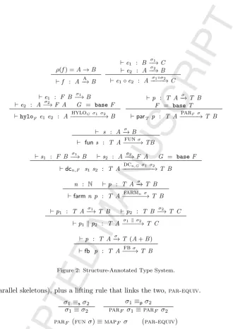
Figure 2: Structure-Annotated Type System.
parallel skeletons), plus a lifting rule that links the two,par-equiv.
σ1≡sσ2 σ1≡σ2
σ1≡pσ2
parF σ1≡parF σ2
parF (funσ)≡mapF σ (par-equiv)
In [9], we have defined a number of equivalences, using well-known properties of skeletons (e.g. [2, 7]) plus fundamental hylomorphism laws [31]. For example, a parallel pipeline structure (k) is functionally equivalent to a function compo-sition; a task farmfarm can be introduced for any structure; and divide-and-conquerdcand feedbackfbskeletons can both be derived from hylomorphisms.
funσ1kfunσ2 ≡p fun(σ2◦σ1) (pipe-equiv)
dcn,F σ1 σ2 ≡p fun(hyloF σ1 σ2) (dc-equiv)
farmn σ ≡p σ (farm-equiv)
fb(funσ) ≡p fun(iterσ) (fb-equiv)
3.4. Automatic Rewriting using Cost Information
We can use the convertibility relation to define arewriting systemthat allows us to automatically rewrite functionally equivalent structured parallel forms. We interpret structured expressions and parallel processes as members of families of functionally equivalent expressionsEs, indexed by a representative structured expression s. For all well-typed s : A 7−→σ B, σ is an index of the family defined by s, i.e. φs(σ) ∈ Es. The function φs : Σ → Es is a partial func-tion whose result is defined for any structureσ that is an index of the family
Es. The type-checking algorithm needs to decide whether rewriting s to the desired structure would result in a member of the familyEs. We achieve this by defining a confluent rewriting system on structures, Σ Σ [9]. Since, for a given s, the family Es is finite, we can use cost information to find optimal
structures. For small enough parallel structures, exhaustive search is feasi-ble. For larger structures, we can equip a family Es with a strong ordering
σ1, σ2 ∈dom(φs), σ1 ≤ σ2 iff cost(σ1) ≤ cost(σ2), and use this ordering to optimise the search process, at the cost of not necessarily finding an opti-mal structure1 In order to exploit this technique, we must provide a cost model that is strongly connected to our execution semantics. This is the focus of the remainder of this paper.
4. An Operational Semantics for Queues
In order to obtain a sound cost model, we need to first give an operational semantics for each of our skeletons, and derive then cost information from this semantics. We will build our skeleton semantics (Sec. 5) on a small-step trace-based operational semantics for the queues that are used to link these skeletons. Each step in the queue semantics will describe a state transition within a simple parallel process abstraction. We first give a number of basic definitions.
State. Astate comprises a tuple of three main structures,W × Q × S:
• an environment of worker definitions,W, which is a mapping from worker identifiers to worker loopdefinitions, i.e. to the code that is run by each worker of the parallel process;
• an environment ofworker states,S, which represents the instruction that is currently being executed by the worker; and,
• aqueue environment,Q, which represents the buffers that link the workers. We will assume that the worker environment, W, is fixed. The rules in our operational semantics therefore have the form:
(Q,S) −→α (Q0,S0)
1We conjecture that a family E
They are given in terms of a labelled state transition system. The labels are the actionsα::=gwq |ew(f, x)| pw(x, q), which respectivelyget an input from a queue,evaluate a functionf on an inputx, orputa result on a queue. Actions are performed on specific queues q, and are tagged with the worker, w, that performs the action.
Queue Environments. A queue environment is a mapping from queue identifiers to sequences of values.
Q =
q. . .0 7→ hx0, x1, . . .i qn 7→ h. . .i
Queue Operations. We assume the usual basic, thread-safe, enqueue and de-queueoperations.
enqueue(Q[q7→vs], x, q) → Q[q7→ hx|vsi]
dequeue(Q[q7→ hvs|xi], q) → Q[q7→vs], x
We overload the notation forenqueue/dequeue operations to also work on sums and products. Enqueuing a product type value into a “product queue” results in a pairwiseenqueue on each sub-queue. Enqueuing a sum type value into a “sum queue” yields a singleenqueueoperation, on the corresponding queue. We useQto refer to these queue structures, and qto refer to queue identifiers.
Q ::= q|q1× · · · ×qn |q1+· · ·+qn
We interpret the enqueue operation on products of queues as a sequence of simpleenqueue operations:
enqueue(Q, q1× · · · ×qn,(x1, . . . , xn))
= enqueue(enqueue(. . .enqueue(Q, q1, x1). . .), qn, xn)
Anenqueue on a sum of queues is anenqueueon the corresponding queue. For example, if 0≤i≤n:
enqueue(Q, q1+· · ·+qn,inj1 x) =enqueue(Q, qi, x)
Dequeueoperations work similarly. We interpret thedequeueoperation on prod-ucts of queues as a sequence of simpledequeue operations:
dequeue(Q, q1× · · · ×qn) = (dequeue(Q, q1), . . . ,dequeue(Q, q1)) Adequeueoperation on a sum of queues dequeues an element from the first non-empty queue. For example, if 0≤i≤n, and for all j, 0≤j < i, Q[qj 7→ hi],
andQ[qi7→ hvs|xi], then:
dequeue(Q, q1+· · ·+qn) =inji (dequeue(Q, qi))
This is a purely arbitrary choice. Any alternative ordering (e.g. round-robin) is equally acceptable. In the operational semantics, each action will represent an
enqueue ordequeue operation on a single queue. So dequeuing from a tuple of
Workers. In each iteration, a worker first performs a sequence ofdequeues, then performs its local computation,f, and finally performs a sequence of enqueue
operations. We represent this as:
W=
w7→worker· · ·(Qi, f, Qo)
· · ·
where Qi and Qo are the input and output queue structures. The example
below shows the state of a worker that is in the process of dequeuing from a tuple of queue identifiers, and that has already dequeued n elements from the firstnqueues:
S =
w7→(x1, . . . , xn,dequeue· · ·(qn+1), . . . ,dequeue(qm))
· · ·
Generally, a worker state can be either a sequence (or sum) ofdequeue/enqueue
operations, or aneval operation. Let v be a value:
st ::=inSt | outSt | eval(x)
inSt ::=v | dequeue(q) | (inSt, . . . ,inSt)
outSt ::=v | enqueue(q, x) | outSt;. . .;outSt
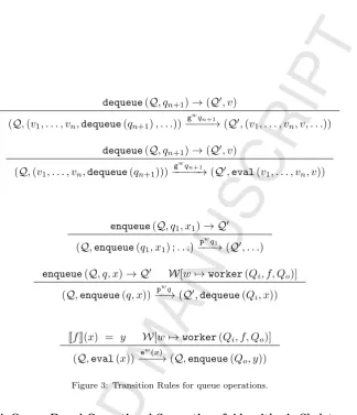
The transition rules for our operational semantics are given in Figure 3. Note that we overloadenqueue/dequeue operations to also deal with sums and prod-ucts. We also assume that enqueues on simple queues are trivial. It is now straightforward to define the operational semantics on a sequence of workers:
(Q,st)−−→αw (Q0,st0)
(Q,S[w7→st])−−→αw (Q0,S[w7→st0])
It is easy to see that the only rules that affect the output are those involving communication (enqueue/dequeue).
Definition 4.1 (Ready and Idle State). A worker w 7→worker(Qi, f, Qo) is
in a readystate if it is at the beginning of its worker loop. A worker is idle if it is ready and there are no inputs in its input queue structureQi
dequeue(Q, qn+1)→(Q0, v)
(Q,(v1, . . . , vn,dequeue(qn+1), . . .)) gwq
n+1
−−−−−→(Q0,(v
1, . . . , vn, v, . . .))
dequeue(Q, qn+1)→(Q0, v)
(Q,(v1, . . . , vn,dequeue(qn+1))) gwqn+1
−−−−−→(Q0,eval(v
1, . . . , vn, v))
enqueue(Q, q1, x1)→ Q0
(Q,enqueue(q1, x1) ;. . .) pwq1
−−−→(Q0, . . .)
enqueue(Q, q, x)→ Q0 W[w7→worker(Q
i, f, Qo)]
(Q,enqueue(q, x)) p wq
−−→(Q0,dequeue(Q
i, x))
[[f]](x) = y W[w7→worker(Qi, f, Qo)]
(Q,eval(x)) e w
(x)
[image:15.595.151.476.98.476.2]−−−→(Q,enqueue(Qo, y))
Figure 3: Transition Rules for queue operations.
5. A Queue-Based Operational Semantics of Algorithmic Skeletons
We can now build the parallel structures that we require.
Parallel Composition of Processes. We define the parallel composition of pro-cesses as the union of their queues and workers.
(W1,Q1,S1)k(W2,Q2,S2) = (W1] W2,Q1∪ Q2,S1] S2)
Worker. We lift sequential functions into workers with input and output queue structures. The new worker isready.
qfun(f)(Q0, Q1) =
W= [w7→worker(Q0, f, Q1)],Q=Q0∪Q1,S= [w7→dequeue(Q0)]
Task farm. A task farm replicates a structurentimes:
qfarm(n,P)(Q0, Q1) =
ntimes
z }| {
P(Q0, Q1)k. . .k P(Q0, Q1)
Parallel pipeline. A parallel pipeline is the parallel composition of two struc-tures, linked by an intermediate queue. Letqbe a fresh queue identifier:
Feedback loop. A feedback loop is created by simply inspecting the output of a structure, and placing it back in the input queue depending on the result:
qfeedback(P)(Q0, Q1) =P(Q0, Q0+Q1)
Parallel Hylomorphism. One of the novelties of this paper lies in describing how to parallelise an arbitraryhylomorphism using a divide-and-conquer skeleton. We will first describe a series of simple semantics-preserving transformations for any hylomorphism. The idea is that if the anamorphism part of a hylo-morphism needs to split an input value into at most n sub-values, then we will create n+ 1 queues, the first of which will send the corresponding input to the “combine” worker, and the remaining n of which will send the subdi-vided inputs to the subsequent divide stages. If an input cannot be disubdi-vided any further, then a synchronisation token, 1, will be sent. Given a functor F
described as a combination of sums, products and constants,F A = T,where
A is nested at mostntimes within a product in T, we define the functor DF
asDF B= (1 +T[1/A])×
n times
z }| {
(B× · · · ×B).If we can convert any hylomorphism to this new structure, then we can use its regular structure to create a regular “divide-and-conquer graph” with the following communication structure:
1. The divide worker will communicate a value of type 1 +T[1/A] to the corresponding combine worker, and values of type B to the subsequent
divide workers.
• A value of type 1+T[1/A] contains the “non-recursive” part ofT, plus a unit to indicate that the input could not be divided any further. • A combine worker can use a value of this type to decide how to
recombine the n values of type B that has been received from the previous stages of the divide-and-conquer skeleton.
2. Adivide worker takes an element of type 1 +A. If it is 1, then it transmits
inj1() to all its output queues. This indicates to the subsequent workers that there is no more work to be done. If it receives a value of typeA, it divides it, splits the recursive and non-recursive parts ofT, and sends the corresponding elements to the output queues.
3. Acombineworker that receives an element of type 1 from the correspond-ingdivide worker will simply discard all values received from the previous level, and send 1 to thecombine worker of the next level. If it receives an element of typeT[1/A], it will need to recombine the corresponding value of typeF Afrom the inputs, and apply thecombine function to it.
We need a way to change a hylomorphism from anF structure to DF. Note
that there are two functions
d : 1 +F A→DF (1 +A)
Thedfunction separates the occurrences of values of typeAin some structure
F A into the corresponding T[1/A] and n-tuple of 1 +A, and the function c
recomposes a structureF A from the structure ofDF. If d receives inj1 (), then it just returns an+ 1 tuple ofinj1(). Thecfunction returnsinj1() if the first component of the tupleDF (1 +A) isinj1(). Note that the typesF and DF are not isomorphic, since the function c ispartial. However, the following
properties do hold:
c ◦ d = id
d ◦ (1 +F f) = DF (1 +f) ◦ d.
Using these properties, we can show that the following condition holds for any functorF:
1 +hyloF g h
=
1 +g ◦ F (hyloF g h) ◦ h
=
(1 +g) ◦ (1 +F (hyloF g h)) ◦ (1 +h)
=
((1 +g)◦c◦d) ◦ (1 +F (hyloF g h)) ◦ (1 +h)
=
((1 +g)◦c)◦ DF (1 +hyloF g h) ◦ (d◦(1 +h))
=
hyloDF ((1 +g)◦c) (d◦(1 +h))
Using this, we can convert to a hylomorphism of a different structure. For all
hyloF g h : A→B, given any x : B, then
xOid◦(hyloDF ((1 +g)◦c) (d◦(1 +h))) ◦ inj2 =
xOid◦(1 +hyloF g h) ◦ inj2
=
(x◦1)O(id◦hyloF g h) ◦ inj2 =
id◦hyloF g h
=
hyloF g h
This shows that the first level of a divide-and-conquer must wrap the input in
inj2, and the last level of a divide-and-conquer must unwrap the result using
xOid, for any arbitraryx : B. We define these as:
D1(F, h) = d◦inj2◦h C2(F, g) = (1 +g)◦c D2(F, h) = d◦(1 +h) C1(F, g) = (xOid)◦(1 +g)◦c
Although the structure DF may appear to be complicated, it neatly fits our
D1(F, h)
D2(F, h) D2(F, h)
· · · ·
C2(F, g) C2(F, g)
C1(F, h)
q1 q2
q0
1 q02
[image:18.595.199.476.103.345.2]q0
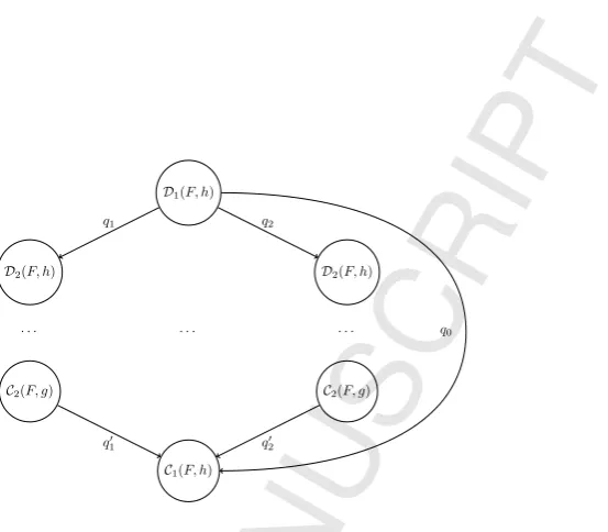
Figure 4: Divide-and-conquer skeleton: theqiare the queues; circles represent the workers.
types (1 +T[1/A]) and 1 +A, and can create workers that split/combine values of these types, as shown in Figure 4. Values of type 1 are simply used to synchronise the differentdivide andcombineworkers, so that the different levels of a divide-and-conquer skeleton can operate on different inputs in parallel. We define this as:
qdc(n, F, g, h)(Q0, Q1) = qdc0(hyloFg h, n, F, g, h, C1, D1)(Q0, Q1)
qdc0(f,0, F, g, h, c, d)(Q0, Q1) = qfun(f)(Q0, Q1)
qdc0(f, n, F, g, h, c, d)(Q0, Q1) =
qfun(d(F, h))(Q0, q0×q1× · · · ×qn)
kqdc0(1 +hyloFg h, n−1, F, g, h,C2,D2)(q1, q01) k. . .
kqdc0(1 +hyloFg h, n−1, F, g, h,C2,D2)(qn, qn0)
kqfun(c(F, g))(q0×q01× · · · ×qn0, Q1)
Soundness. It is obvious from these definitions that the soundness of the oper-ational semantics with respect to the denotoper-ational semantics can be reduced to correctly connecting the queues of the algorithmic skeletons.
6. Predicting Parallel Performance
be realised as an algorithm. In this paper, we are mainly interested in predict-ing realisticlower bounds on the execution times of parallel programs. While the more usual worst-case predictions might be useful for safety reasons, they would not provide sufficient information to enable us to choose the best parallel implementation. Moreover, when “initialisation” and “finalisation” times are taken into account, the worst-case parallel execution time will generally be very similar to the sequential case, and so provide very little insight into parallel performance. The amortised average case timings that we use here are much more useful for predicting the actual parallel performance of the system.
6.1. Costs and Sizes
The sequential components of our algorithmic skeletons are given as suitably lifted functions. Before we can define their cost models, we must first explain how we derive cost models for hylomorphisms. Vasconcelos [46] showed how to use sized types [24] for developing an accurate space cost analysis. Sized types have also been used for estimating upper bounds of execution times of parallel functional programs [28]. The success on using sized types for cost analysis motivated our approach. We exploit this previous research onsized types [46], as well as previous research oncost equations [40]. Acost equationfor a function
f : A→B provides an estimate of the execution time off given an input of a given size.
costf : sizeA→time
To obtain the inputs for these cost equations, we use a variant of the usual notion ofsized types[24]. The only difference is that, since we are interested in amortised costs, we useaverage sizes rather than upper or lower bounds. The notion of average size is dependent on each problem, so rather than defining a generic calculation, we require specific definitions for each function andtype constructor. Suitable definitions include, e.g. the average depth of a tree, the average number of elements in a structure etc.
Type Constructors. These are either constant typesC, or recursive types defined as the fixpoint of some base functorµF.
Sizes and Size Constraints. We reuse the idea of stages [5]. Essentially, sizes are either size variables or sums of sizes, and size constraints are inequalities on sizes. We writeAi
|C for a sized typeAwith size iand constraintC.
Sized types. We require the basic polynomial (bi-) functors to be annotated with size expressions for each alternative (given as a sum-type). For example, the base bifunctor of a binary tree can be annotated as follows:
F0∨1+i+j A B = 1 +A×Bi×Bj
of sizej. Note that there are alternative definitions for the size of a functor
F, e.g: F1∨max(i,j) A B = 1 +A ×Bi
×Bj. In a more general sense, a
sized-type is a type constructor that is annotated with size information, e.g.
Inti, Listj+k A, . . .. Thein
F andoutF functions for a sized base functor of a
recursive type must have the following type and constraints:
inF : FjµF→µiF |i=j
outF : µiF →FjµF |i=j
That is, we require that the sizes of the base functor represent the same infor-mation as the sizes of the recursive type. Finally, we will use|A|to denote all the nested size information and size constraints in a typeA. This is useful for defining cost models that require access to nested size information.
Deriving Recurrences from Hylomorphisms. We now show how we use sized types to derive recurrences. Essentially, we will define acost equation for each syntactic construct, that takes some cost equation parameters and produces another cost equation. Although the cost of a function is not, in general, com-positional, since it may depend on previous computations as well as on other properties of the input data, we will here take a compositional approach under the assumption that only the sizes will affect the execution times. This is a valid way to obtainamortised costs. The execution time of each primitive oper-ation is assumed to be a constant that depends on the target architecture. This must be provided as a parameter. The cost of a function composition is the sum of the run-times of each stage, plus some architecture-dependent overhead. The only difficult case involves recursive functions. For recursive functions that are defined as hylomorphisms, we generate recurrence relations, as with Bar-bosaet al. [4]. In a similar sense to Sands’ work [40], our cost equations can be thought of as functions that we are integrating into our type-system. For example, assuming that we have the following sized-type forquicksort:
merge : T0∨1+i+jA(ListA)
→ Listk A|k= 0 ∨ k=i+ 1 +j split : Listn A → T0∨1+r+sA(ListA)
| n= 0 ∨ n= 1 +r+s
qs : Listi A → Listj A|i=j qs = hyloT merge split
Given suitable cost equations for split and merge, costsplit, costmerge, then there are two cases. Eithern= 0, in which caset= 0, so we assume some time
costsplit(0) +costmerge(0), orn= 1 +r+s, in which case:
costqs =costsplit(1 +r+s) +costmerge(r+ 1 +s) +costqs(r) +costqs(s)
into account would, of course, require further programmer input.
costqs(n) =
costsplit(1 +r+s) +costmerge(r+ 1 +s) +costqs(r) +costqs(s) wherer= (n−1)/2 ands= (n−1)/2
We simplify this internally to generate the desired recurrence relation:
costqs(0) =costsplit(0) +costmerge(0)
costqs(n) =costsplit(n) +costmerge(n) + 2×costqs((n−1)/2)
6.2. Costing Traces of Parallel Processes
We now describe a systematic way to derive cost equations. We start with a structureC, with some initial emptyPiand costci. Taking suitably sound
sim-plifications and approximations oftime(α1, . . .), we then derive an “amortised cost equation” costC such that for all input l with sized-type hAii and trace,
C(P1, . . . ,Pn)(qin 7→ l, qout 7→ hi) α1,...
−−−→ C(P1, . . . ,Pn)(qin 7→ hi, qout 7→ l0),
theni×costC(c1, . . . , cn)|A| ≈ time(α1, . . .).We differentiate three phases in the execution of a parallel process: aninitialisation phase, asteady state, and a finalflushing phase. For example, a pipeline of two atomic functions, w1 kw2, reaches a steady state after executing the initialisation phase of w1. At this point,w2 can run in parallel withw1:
qq01 7→ h7→ hix,1, x2, . . .i, q2 7→ hi
,
w1 7→worker(q0, f, q1) w2 7→worker(q1, g, q2)
gw1q0,ew1x1,pw1q1
−−−−−−−−−−−−−→
qq01 7→ h7→ hxf x2, . . .1i, i, q2 7→ hi
,
w1 7→worker(q0, f, q1) w2 7→worker(q1, g, q2)
We capture these ideas in the definitions below.
Definition 6.1(Steady State). A parallel processP is in a steady state,steady(P), if for allw∈ P,¬idle(w).
Definition 6.2 (Initialisation Phase). The initialisation phase for a paral-lel process initial(P1) is the shortest sequence of a1, a2, . . . , an, such that if
P1
a1,a2,...,an
−−−−−−−→ P2, then steady(P).
Definition 6.3(Flushing Phase). The flushing phase for a parallel processP1
is the sequence ofa1, a2, . . . , an, such that for alli∈[1. . . n]and for allw∈ P1, ai6=dequeue(qin)w, and ifP1
a1,a2,...,an
cost(funσn,m) =T
enqueue(n) +costi+Tdequeue(m)
where|σ|=i→j|C
cost(farm n σi,o) =cost(σi×n,o×n)
n cost(σi,j1 kσ
k,l
2 ) = max
n
cost(σ1i,j+k),cost(σ
j+k,l
2 )
o
cost(fbσn,m) =if(|σ|= 0)
then cost(σn+m,m)
else cost(σn+m,m) + cost(fb(resize(σn,m,|σ|)))
cost(dcn,F σ1 σ2) = max
cost(D(F, σ2)),
cost(dcn−1,F σ1σ2),
cost(C(F, σ1))
Figure 5: Cost equations.
Total Cost and Amortised Cost:. Given some initial P and final P0, where P α1,...,αn
−−−−−→ P0, the total cost of a parallel computation is time(α
1, . . . , αn).
The cost of each action depends on the worker environment. Based on [21], we calculate the queue contention on each queue by simply counting the number of workers in which a queue appears inW. Then, the cost of thegwandpwis ad-justed according to the corresponding overhead. If we split the trace intoP−−−→init P1
steady
−−−−→ P2 −−−→ Pflush 0, where init = α1, . . . , αi, steady = αi, . . . , αj,
flush = αj, . . . , αn such thatinitial(P), steady(P1),and final(P0) then the total time is:time(α1, . . . , αn) =time(init)+time(steady)+time(flush).
We can systematically derive cost models fortime(init) andtime(flush) using the method shown below.
6.3. Deriving Cost Equations from the Operational Semantics
We now show how to systematically derive the cost equations in Figure 5 from our operational semantics for skeletons. We base our approach on symbolic ex-ecution. The following assumptions are used to automatically derive amortised cost equations for our parallel structures.
1. The queues contain enough elements for eachdequeue to succeed.
2. Each time an element is dequeued, we will return a size that is extracted from its type.
3. Evaluating a function on a size immediately returns the size of the output type of that function, plus the set of constraints that relate the input and output sizes.
5. Any substructure (e.g. a farm worker) produces a trace that can be safely interleaved with the trace that is produced by other substructures (i.e. without modifying the result of the overall computation), and that has a known cost.
Note that assumption 1 holds only for asteady structure, so these cost equa-tions would not be useful for estimating run-times of a computation where
time(init) and/ortime(flush) dominate.
Worker cost. A worker, w, computing f : Ai → Bj | C in environment
W[w7→worker(qi, f, qo)] produces the “symbolic trace”: gwqi, ew |Ai|, pwqo.
Assuming there exists some trace α1, . . . , αn that can be safely interleaved
with this trace, we want to know the cost of the actions in α1, . . . ,gwqi, . . .,
ew i, . . . ,pwqo, . . . , αn. Here, the cost of gwqi will depend on any other action
that is happening in parallel. The only actions that can affect the cost of a queue operation are other queue operations that are acting on the same queue. Ifn is the number of workers wget ∈ W such thatwget 6=wi and the number
of workers operating onqo ism, then if we assume that the cost of theenqueue
anddequeue operations is as described by [21], then the cost is:
time(gwqi, ew i, pwqo) = Tenqueue(n) +costf(i) +Tdequeue(m)
We associate this cost with the corresponding high-level structure, so that it can be used by our type-checking algorithm:
cost(funσ) = Tenqueue(n) +cost(σ) +Tdequeue(m)
The parameters n, m and cost(σ) can be instantiated from the context, and added to the structure σ by the type-checking algorithm in a straightforward way. We write σn,m for a structure with n contending workers in the input
queue, and withmcontending workers in the output queue. Note that the real cost, understood as an equation from an input size to an execution time, would be cost(funσn,m)(Ti j) = i
×(Tenqueue(n) +costσ(j) +Tdequeue(m)), if we
assume thatT containsielements of sizej. Since we can annotate structures,
σ, with sizes, we can abuse our notation for extracting sizes of types,|σ|, and “overload” the meaning ofcostto take a structure and yield an amortised cost.
Farm cost. A farm,C(Q0, Q1)k · · · k C(Q0, Q1), consists of a number of paral-lel processes that are joined using our paralparal-lel composition operator, and that share input and output queues. Since we symbolically evaluate theenqueueand
dequeue operations, we can takenarbitrary traces, one for each farm worker:
C(Q0, Q1)
α1 1,α12,...
−−−−−→ P0, . . . , C(Q 0, Q1)
αn 1,αn2,...
−−−−−−→ P0
Each trace has costci, . . . , cn. To obtain amortised costs, we assume that each
considers the queue contention, we simply need to calculate the maximum cost of any worker, assuming that each sub-trace can be performed in parallel:
time(αia, α j
b, . . .) = max
time(α1
1, α21, . . .),
time(. . .), time(αn
1, αn2, . . .)
= max{c1, . . . , cn} = c
Note that if eachP producesk outputs, thenqfarm(n,P) producesk×n out-puts. So, in order to obtain an amortised cost, when we associate it with the high-level structure, we need to divide the total cost byn.
cost(farm n σ) = cost(σ)
n
Note that, although this cost is obviously correct, the main point is that it was
systematically derived from the simple queue-based model. It is thus sound by construction, and so no longer needs to be a parameter of our type system.
Parallel pipeline. A pipeline,C1(Q0, q)k C2(q, Q1), consists of two parallel pro-cesses that are joined using our parallel composition operator, and connected using an intermediate queueq. Again, we take a similar reasoning process:
C1(Q0, q)
α11,α 1 2,...
−−−−−→ P1 C2(q, Q1)
α21,α 2 2,...
−−−−−→ P2
Assume costsc1,andc2for each process:
time(αia, α j
b, . . .) = max
time(α1
1, α12, . . .),
time(α21, α22, . . .)
= max{c1, c2}
Note that, in order to accurately lift these costs to the high-level structures, we need to consider the size of the output ofα1
i, not the size of theα2j input.
We do this by writingresize(σ2,|σ1|), meaning that the input ofσ2is altered to have the size of the output size in |σ1|. We can do this safely since our type-checking algorithm can ensure that sizes meet the necessary constraints. Finally, we associate the cost with the corresponding high-level structure:
cost(σ1kσ2) = max{cost(σ1),cost(resize(σ2,|σ1|))}
Feedback loop. A feedback loop requires us to take into consideration that an element may be written back to the input queue,C1(Q0, Q0+Q1). The structure Cmust compute some functionf, and we require it to have type:
Fn∨0A = An+B, s.t. f :Ai →F Aj |j < i.
C1(Q0, Q0+Q1)
α11,α 1 2,...
−−−−−→ P1 will need to be taken ntimes to ensure that, on average, at least one element is enqueued into output queueQ1.
C1(Q0, Q0+Q1)
α11,α 1 2,...
−−−−−→ P1
...
−→ Pn
Since this parameter can be estimated from the sized types, we can again assume that a structureσis parameterised on it, and can use this in our high-level cost models. Again, we need to useresizeto generate the appropriate cost equation:
cost(fbσ) = if (|σ|= 0)
then cost(σ)
else cost(σ) + cost(fb(resize(σ, σ)))
Divide-and-Conquer. The divide-and-conquer skeleton requires a little more work, since we first need to transform the structure so that it matches the skeleton. Since this transformation can be done in a fairly standard way, we initially focus on the cost of the divide-and-conquer skeleton:
qdc0(0, F, g, h)(Q0, Q1) = qfun(1 +hyloFg h)(Q0, Q1)
qdc0(n, F, g, h)(Q0, Q1) = qfun(D2(F, h))(Q0, q0×q1× · · · ×qm)
kqdc0(n−1, F, g, h)(q1, q10) k. . .
kqdc0(n−1, F, g, h)(qm, qm0 )
kqfun(C2(F, g))(q0×q10 × · · · ×q0m, Q1)
Since we define this skeleton inductively for some “depth”n, we start with the base case (depth 0), which is equivalent to the cost of an atomic function:
cost(dc0,F σ1σ2) = cost(fun(hyloF σ1 σ2))
For the recursive case, we assume 2 +m traces, one for each “recursive” case, plus the trace of the divide and the trace of the combine parts. Again, we assume that the traces can be safely interleaved, so we can calculate the cost of the total trace as:
time(α1, . . .) = max
time(αdiv, . . .),
time(αqdc, . . .),
time(. . .), time(αqdc, . . .),
time(αconq, . . .)
= max
time(αdiv, . . .),
time(αqdc, . . .),
time(αconq, . . .)
again useresize, we assume that the actual sizes have been correctly updated in thedc structure:
cost(dcn,F σ1 σ2) = max
cost(D(F, σ2)),
cost(dcn−1,F σ1 σ2),
cost(C(F, σ1))
7. Examples
This section a) illustrates the cost equations that can be derived from some parallel structures, as they are inferred by the type system; and,b) compare the costs that are obtained by cost models for some simple structures with actual runtimes, in order to provide evidence for the feasibility of our approach.
7.1. Type-based Derivation of Cost Equations 7.1.1. Image Merge
Image merge basically composes two functions: mark and merge. It can be directly parallelised using different combinations of farms and pipelines.
imn = parL (m1kfarmnm2)
imgMerge : Listk(Img×i+jImg) 7−−−→imn Listk(Imgmax(i,j))
imgMerge = mapList (merge ◦ mark)
The type system tries the following substitutions form1and m2in im:
δ ={m1 ∼ fun a, m2 ∼ fun a}
δ1={m1 ∼ farm n1 (fun a), m2 ∼ farm n2 (fun a)} δ2={m1 ∼ fun a, m2 ∼ farm n2 (fun a)} δ3={m1 ∼ farm n1 (fun a), m2 ∼ fun a}
δ4={m1 ∼ fun a, m2 ∼ fun a}
Note that the substitutions that introduce a farm tom2would yield a structure
farm n(farm n2) . In our model, this would not be a problem, since the un-derlying structure would be equivalent tofarm (n×n2) . We could improve our type-checking implementation by considering the context of a metavari-able. This would avoid superfluous rewritings. In our example, we assume that
sz = [d]1000. This represents the size of 1000 pairs of images of ddimensions. Arithmetic operations onsz are applied to the superscript. The size function of the first stage|ac1| is the identity, since we are not modifying the images. The
parameters for the number of farm workers are fixed to be those with the least cost, given some maximum number of available cores. For δ1, we determine thatn1= 9,n = 3 andn2= 5. The values of the costs on those sizes, and the overheads of farms and pipelines are given below. In the example cost equation below,|ac1|(sz) denotes the output size of the first stage, obtained usingresize,
omit these numbers and just assume a 24-core machine with similar overheads for farms, pipelines, divide-and-conquer and feedbacks.
c1 [(2048×2048,2048×2048)]n = ×25.11ms
c2 [(2048×2048,2048×2048)]n = ×45.21ms κ(9) = 29.66ms κ(15) = 60.93ms
cost (δ1im(n))sz
= max{c1 (
sz n1
) +κ(n1+n2), c2(|
ac1|(sz)
n2
) +κ(n1+n2)}= 3145.69ms
cost (δ2im(n))sz = 25123.81ms
cost (δ3im(n))sz = 3189.60ms
cost (δ4im(n))sz = 25123.81ms
The structure that results from applying δ1 is the least cost one, δ1(im2(3)), withn1= 9 andn2= 5.
7.1.2. Quicksort
We will now analysequicksort and show how it can exploit a divide-and-conquer parallel structure. Our cost models show the following estimations, whereκis adjusted to take into account the overheads of adcstructure, again calculated as the cost of the queue contention. In this example, we set the size parameter of our cost model to 1000 lists of 3,000,000 elements:
qsorts : List(ListA)7−→List(ListA)
qsorts = mapList (hyloF A merge div)
cost (parL(dcn,F ac1 ac2))sz
= max{c2 (|ac2| isz), . . .
,cost(hyloF ac1 ac2) (|ac2|
nsz), . . .
,max{c1(|ac1| i|a
c2|
nsz)} = 42602.72ms
cost (parL(farmn (fun(anaLac2))k(fun(cataL ac1))))sz
= 27846.13ms
cost (parL(farmn (fun(hyloF ac1 ac2))))sz
= 32179.77ms . . .
Since the most expensive part of thequicksort function is thedivide, and since flattening a tree is linear, the cost of adding a farm to the divide part is less than the cost of using a divide-and-conquer skeleton for this example.
7.1.3. N-Body Simulation
represent the eight octants of the space. The leaves of the tree contain the bodies. We then calculate the cumulative mass and centre of mass of each region of the space. Finally, the algorithm calculates the net force on each particular body by traversing the tree, and updates its velocity and position. This process is repeated for a number of iterations. We will here abstract most of the concrete, well known details of the algorithm, and present its high-level structure, using the following types and functions:
C = Q×Q
F A B = A + C×B8
G A = F Body
Octree = µG
insert : Body×Octree→Octree
Since this algorithm also involves iterating for a fixed number of steps, we define iteration as a hylomorphism, as well as its structure.
loop : Σ→Σ
loopσ = hylo(+) (idOσ) ((a+ (aM(a◦a)))◦(a◦a?))
loopA : (A7−→m A)→A×N loopm 7−−−−−−→A
loopA s =
hylo(A+) (id Os)
((π1+ (π1M((−1)◦π2)))◦((== 0)◦π2)?)
This example uses some additional functions: calcMass annotates each node with the total mass and centre of mass; dist distributes the octree to all the bodies, to allow independent calculations,calcForcecalculates the force of one body; andmoveupdates the velocity and position of the body.
calcMass : G Octree→G Octree dist : Octree×ListBody
→L(Octree×Body) (Octree×ListBody) The algorithm is:
nbody : ListBody×N loopσ
7−−−−−→ListBody
nbody = loop(anaL (L (move◦calcForce)◦dist)
◦((cataG (inG◦calcMass)◦cataLinsert)Mid))
Note that we do not allow the fixed structure determined byloopto be rewrit-ten. Even if we were to allow this, there is a data dependency in its definition that suggests that no parallelism can be extracted from it. However, the loop body does contain sources of parallelism, which our type system is able to ex-ploit. In particular, the structure of the loop body is:
σ=anaL(L(a◦a)◦a)◦(cataG(in◦a)◦cataLa)Mid
The normalised structure reveals more opportunities for parallelisation:
After normalisation, this structure is equivalent to:
σ=parL(fun(a◦a))◦
The structure makes it clear that there are many possibilities for parallelism using farms and pipelines. As before, parallelism can be introduced semi-automatically using our cost models. For example, setting the input size to 20,000 bodies:
σ =parL(farmn k )◦
σ0=parL(min cost( k ))◦
cost(fun ac1kfun ac2)sz = 310525.67ms
cost(farm6 (fun ac1)k(fun ac2))sz = 55755.43ms
cost(fun ac1kfarm1 (fun ac2))sz = 310525.67ms
cost(farm20(fun ac1)kfarm4(fun ac2))sz = 15730.46ms
7.1.4. Iterative Convolution
Image convolution is also widely used in image processing applications. We as-sume the typeImgof images, the type Kern of kernels, the functor F A B =
A+B×B×B×B, and thesplit, combine, kern andfinished functions. The
splitfunction splits an image into 4 sub-images with overlapping borders, as required for the kernel. Thecombine function concatenates the sub-images in the corresponding positions. Thekernfunction applies a kernel to an image. Fi-nally, thefinishedfunction tests whether an image has the desired properties, in which case the computation terminates. We can represent image convolution on a list of input images as follows:
conv : Kern→(ListImg7−→σ ListImg)
conv k =
mapList (iterImg (finished?◦hyloF (combine◦F (kern k)) (splitk)))
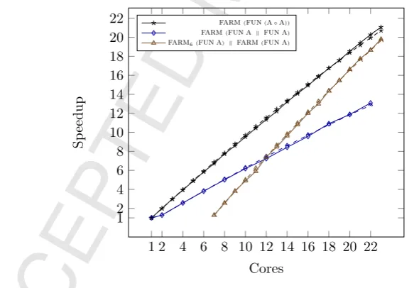
σ = parL (fb(dcn,L,F (a◦F a)ak )) = parL (fb(farm n k k )) = min cost(parL(fb( k ))) = . . .
cost (parPL (fb(ac1 kac2))) sz =
1≤i,|ac1kac2|isz>0
cost (ac1kac2) (|ac1 kac2| isz)
= 20923.02ms
cost (parL (fb(farm4 (fun ac1)k(fun ac2))))sz
= 6649.55ms
cost (parL (fb(fun ac1 kfarm1 (fun ac2))))sz
= 20923.02ms
cost (parL (fb(farm14 (fun ac1)kfarm4(fun ac2))))sz
= 2694.30ms . . .
Collectively, these four examples have demonstrated the use of our techniques for all the parallel structures that we consider in this paper. In the next section, we provide evidence to validate the cost models that we have derived from our operational semantics against actual parallel executions.
7.2. Actual vs Predicted Speedups
In order to validate our results, we have compared predicted versus actual speedups for a number of example parallel programs. Our results not only vali-date our cost equations, but also confirm our previous experimental results [21]. We have taken the results of type-checking a number of examples, and im-plemented the corresponding structures in C, following our model, using the
pthreads-based queue implementation that we described in [21]. In Section 6.3, we showed that most of the cost equations can be simplified to the expected ones, apart from the cost of afun σ structure. Basically, the idea is that the overhead of the parallel structures can be safely pushed down into its workers. We show here how that overhead cost affects the actual runtimes, comparing this with the predicted speedups for some of our parallel structures.
We use two different real multicore machines: titanic, a 800MHz 24-core, AMD Opteron 6176, running Centos Linux 2.6.18;and lovelace, a 1.4GHz 64-core, AMD Opteron 6376, running GNU/Linux 2.6.32.All the speedups shown here have been calculated as the mean of ten runs. Figure 6 shows the real
vs. predicted speedups for task farms, using a simple matrix multiplication
1 2 4 6 8 10 12 14 16 18 20 22 1
2 4 6 8 10 12 14 16 18
nWorkers
Sp
eedup
farmn (funσ)
[image:31.595.191.472.109.391.2]N = 1024 N = 2048
Figure 6: Speedup (solid lines) vs prediction (dashed lines). Matrix Multiplication of matrices of sizes N×N (titanic).
1 2 3 4 5 6 7 8 9 10 11 12
2 3 4 5 6
n Workers
Sp
eedup
farmn (funσ1kfunσ2)
Figure 7: Speedup (solid lines) vs prediction (dashed lines). Image Merge, 500 input tasks (titanic).
[image:31.595.125.428.427.669.2]1 2 4 6 8 10 12 14 16 18 20 22 1
2 4 6 8 10 12 14 16 18 20
n2 Workers
Sp
eedup
farmn1(funσ1)kfarmn2(funσ2)
n1= 1
n1= 2
n1= 4
n1= 6
[image:32.595.193.473.106.392.2]n1= 8
Figure 8: Speedup (solid lines) vs prediction (dashed lines). Image Convolution, 500 input tasks (titanic).
1 2 4 6 8 10 12 14 16 18 20 22 1
2 4 6 8 10 12 14 16 18 20 22
Cores
Sp
eedup
farm(fun(a◦a)) farm(fun akfun a) farm6 (fun a)kfarm(fun a)
Figure 9: Speedup (solid lines) vs predicted (dashed lines). Different Parallel Structures for Image Convolution, 500 Images 1024 * 1024:titanic
[image:32.595.139.431.424.627.2]1 4 8 16 24 32 40 48 56 64 1
4 8 12 16 20 24 28 32 36 40 44 48 52 56
Cores
Sp
eedup
[image:33.595.193.479.108.370.2]farm(fun(a◦a)) farm(fun akfarm4 (fun a)) farm(fun akfun a) farm12 (fun a)kfarm(fun a)
Figure 10: Speedup (solid lines) vs predicted (dashed lines). Different Parallel Structures for Image Convolution, 500 Images 1024 * 1024:lovelace.
8. Related Work
There have been a few previous treatments of parallelism using types, but these deal only with sizes and productivity. One line of work usessized types [24] to incorporate a notion of the sizes of streaming data into a type system. This has been extended to cover a small number of skeletons in the Eden dialect of Haskell [37]. More recently, L´opez et al [29] have presented a type-based methodology, inspired by session types, for verifying that parallel MPI programs follow some given protocol. This approach provides a scalable methodology to statically guarantee that a program satisfies a number of interesting safety prop-erties, such as the absence of deadlocks. Both approaches show that types are indeed useful to prove a number of interesting properties of parallel programs, e.g. termination and productivity. In contrast, our work focuses on the different, but equally important, properties of semantic equivalence and cost.
The expressive power of hylomorphisms for parallel programming was first explored by Fischer and Gorlatch [12], who showed that a programming lan-guage based on catamorphisms and anamorphisms isTuring-universal. The idea of using hylomorphisms for parallel programming also appears in Morihata’s work [33]. Morihata explores a theory for developing parallelisation theorems based on thethird homomorphism theoremandshortcut fusion, and generalises it to hylomorphisms. In contrast, our work directly exploits the properties of hylomorphisms, in order to choose a suitable parallel skeleton implementation for hylomorphisms. The two lines of work are therefore orthogonal, and we can potentially benefit from Morihata’s results in our future work.
the Bird-Meertens Formalism are amongst the many techniques that have been explored [18, 22, 23, 26, 30, 32, 34, 39, 42, 41]. The third homomorphism the-orem states that if a function can be written both as a left fold and a right fold, then it can also be evaluated in a divide-and-conquer manner [16]. This theorem has been widely used for parallelism [10, 14, 15, 17, 27, 33, 35]. The majority of this work enables suitable automation and derivation of efficient parallel implementations. Our work differs in that we allow part of the parallel structure to be chosen in an automated way. This adds flexibility, enabling a parallel implementation to be changed quickly and easily by changing only a single type annotation. One possible extension of our work is to include some automatic transformations derived from the third homomorphism theo-rem. By parameterising our type system over some cost function on parallel structures, we smoothly integrate the introduction of parallelism with the abil-ity to reason about the run-time behaviour of the parallel program. Skillicorn and Cai [43] have previously shown the utility of such an integration of a cost calculus with derivational software development, illustrating the approach for the Bird-Meertens theory of lists. In this paper, we take this approach one step further by using a more general equational theory based on hylomorphisms. Moreover, our type-based approach introduces new benefits, by providing a mechanism for specifying new parallel structures whose denotational semantics can be described as a composition of hylomorphisms.
In a structured parallelism setting, Janjicet al.[25] define a high-level DSL, the Refactoring Pattern Language (RPL), that aims to represent the parallel structure of a program, and capture its execution time. This DSL is a powerful tool, since it allows suitable parallelisations to be found for a given program, and then to apply them to a real C++ program. There are a number of differences between the approach that is described here and RPL. First, our type-based approach does not need to realise parallelisations as refactoring rules: parallel structures are tied to programs in a systematic way by each syntactic construct. The advantage of our approach is that we can use type information to automat-ically generate parallel code at compile-time. The corresponding disadvantage is lack of flexibility: the RPL approach can be combined with a number of refac-torings that can take into account the user input in a more interactive way. The second important difference is that we use hylomorphisms as an unifying con-struct. This enables us to use the rich theory of hylomorphisms for parallelism. Moreover, we base our approach on a decision procedure that is derived from an equational theory that is both sound and complete w.r.t. the rules of the un-derlying equational theory, and we use a standard type unification algorithm to instantiate parallel structures from sequential code. Finally, our parallel struc-tures and cost models are not built-in, but are derived in a systematic way from an underlying cost model and operational semantics.
Finally, Steuwer et al. [44] generate high-performance OpenCL code from a high-level specification by applying a simple set of rewrite rules, and using Monte-Carlo search to traverse the corresponding search space to find an im-plementation. Our approach provides a way to narrow down this search space, while using cost models to automate the rest of the search. It is, in a sense, more general, since we allow our parallel structures to be easily extended. However, we could benefit from exploiting Steuweret al.’s work in GPU-specific rewriting rules and skeletons.
9. Conclusions
This paper has introduced new formally-based cost models for common algorith-mic skeletons. Unlike previous approaches, these cost models are derived from a formal operational semantics for these skeletons, and consider both queue con-tention and scheduling. Using our approach, we can be sure that our cost models are sound w.r.t. the operational semanticsby constructionand we can automat-ically derive cost equations for newly defined parallel structures. A key aspect of our approach is the use of hylomorphisms, combinations of catamorphisms
andanamorphisms (or fold/unfold operations). We have used hylomorphisms to capture some common patterns of parallelism: task farms, pipelines, divide-and-conquers and feedbacks. As shown in our examples, this single construct is surprisingly powerful, providing a system of canonical representations that is easy to understand and that is also easy to transform.
parallel solutions, that need to take into account only basic, easily obtained, information about the costs of executing sequential operations. The use of a type-level approach avoids the usual separation of analysis from program, al-lowing structures and costs to be directly and accurately associated with the program. In particular, all transformations are performed internally by the type checker and we ensure the preservation of the underlying functional behaviour
simply by construction. Moreover, our concrete results show that our cost mod-els are good predictors for actual parallel performance.
A number of obvious extensions can be made to this work. Firstly, there are a few forms of parallel pattern that we have not yet considered: map (re-duce) and fold are clearly instances of hylomorphisms, but stencil and bulk synchronous parallel patterns, for example, may require deeper thought. Sec-ondly, we could investigate more complex and detailed cost models that take into account even more details of a parallel system. Finally, we believe that hylomorphisms and type structures can form the basis for a good, new parallel programming methodology. We intend to explore this by building our ideas into a new parallel library for Haskell that will enable the automatic introduction of parallelism into normal Haskell programs, under type control.
Acknowledgements
This work has been partially supported by the EU Horizon 2020 grant “RePhrase: Refactoring Parallel Heterogeneous Resource-Aware Applications - a Software Engineering Approach” (ICT-644235), by COST Action IC1202 (TACLe), sup-ported by COST (European Cooperation on Science and Technology), and by EPSRC grant EP/M027317/1 “C3: Scalable & Verified Shared Memory via Consistency-directed Cache Coherence”.
References
[1] M. Aldinucci. Automatic program transformation: The Meta tool for skeleton-based languages. Constructive Methods for Parallel Programming, Advances in Computation: Theory and Practice, pages 59–78, 2002.
[2] M. Aldinucci and M. Danelutto. Stream parallel skeleton optimization. In
Proc. PDCS ’99: IASTED Intl. Conf. on Parallel and Distributed Comput-ing and Systems, pages 955–962, Nov. 1999.
[3] M. Aldinucci, M. Coppola, and M. Danelutto. Rewriting skeleton programs: How to evaluate the data-parallel stream-parallel tradeoff. In Proc. In-ternational Workshop on Constructive Methods for Parallel Programming. Technical Report MIP-9805. University of Passau. Passau, 1998.