Automated static symmetry breaking in constraint satisfaction problems

(1)

AUTOMATED STATIC SYMMETRY BREAKING IN CONSTRAINT SATISFACTION PROBLEMS

Andrew Grayland

A Thesis Submitted for the Degree of PhD at the

University of St. Andrews

2011

Full metadata for this item is available in Research@StAndrews:FullText

at:

https://research-repository.st-andrews.ac.uk/

Please use this identifier to cite or link to this item: http://hdl.handle.net/10023/1718

(2)

Automated Static Symmetry Breaking in

Constraint Satisfaction Problems

Andrew Grayland

School of Computer Science

University of St Andrews

A thesis submitted for the degree of

Doctor of Philosophy

(3)

Abstract

Variable symmetries in constraint satisfaction problems can be broken by adding lexicographic ordering constraints. Existing general methods of gener-ating such sets of ordering constraints can produce a huge number of additional constraints. This adds an unacceptable overhead to the solving process. Meth-ods exist by which this large set of constraints can be reduced to a much smaller set automatically, but their application is also prohibitively costly. In contrast, this thesis takes a bottom up approach to generating symmetry breaking con-straints. This will involve examining some commonly-occurring families of mathematical groups and deriving a general formula to produce a minimal set of ordering constraints which are sufficient to break all of the symmetry that each group describes.

In some cases it is known that there exists no manageable sized sets of constraints to break all symmetries. One example of this occurs with matrix row and column symmetries. In such cases, incomplete symmetry breaking has been used to great effect. Double lex is a commonly used incomplete symmetry breaking technique for row and column symmetries. This thesis also describes another similar method which compares favourably to double lex.

The general formulae investigated are used as building blocks to generate small sets of ordering constraints for more complex groups, constructed by combining smaller groups.

(4)

(5)

Acknowledgements

There are a great many people who are partly responsible for this thesis being submitted. Ian Miguel and Colva M. Roney Dougal have been the two single biggest sources of support, both academic and social, I thank them for this. Undoubtedly, with less energetic and enthusiastic supervisors this thesis would not exist. There are a number of other people who have helped me with interesting discussions. These include Barbara Smith, Chris Jefferson, Alan Frisch, Ian Gent, Peter Nightingale and Tom Kelsey. I would also like to thank my office mates, Andrea, Neil and Lars, who not only made my time in St Andrews fun, but also helped with various aspects of this thesis. I could not have completed this work without the support of the administrative staff in the department, especially Alex Bain and Angela Miguel. One of the main requirements of this project has been access to suitable information systems, and for these I am indebted to the systems staff, especially John McDermott. I would also like to thank Microsoft Research and the EPSRC, who funded me throughout the last three and a half years.

When undertaking a task of this magnitude, having time to relax is as important as the time to work. For this reason I thank my drinking friends and all of the people who I have played football with over the last 3 years.

(6)

Although there have been a number of times throughout researching this thesis I have felt like quitting, these feelings have never been stronger than in the last three months. I would like to thank my wonderful girlfriend for helping me through this time, especially as she had at least as many issues to contend with as I did.

(7)

Publications

A large proportion of the work in this thesis has appeared in publications. All of these publications are jointly authored, but the author of this thesis provided the main contribution to each.

• _{A. Grayland and C. Je}ff_{erson and I. Miguel and C. M. Roney-Dougal.}

Minimal ordering constraints for some families of variable symmetries. The Annals of Mathematics and Artificial Intelligence (to appear). 2009.

• _{A. Grayland and I. Miguel and C. M. Roney-Dougal. Snake Lex: An}

Al-ternative to Double Lex. The 15th International Conference on Principles and Practice of Constraint Programming. 2009.

• _{A. Grayland and I. Miguel and C. M. Roney-Dougal. Confluence of}

Reduction Rules for Lexicographic Ordering Constraints. The Eighth Symposium on Abstraction, Reformulation and Approximation. 2009.

• _{A. Grayland and I. Miguel and C. M. Roney-Dougal. In Search of a Better}

Method to Break Row and Column Symmetries. The Eighth Symposium on Abstraction, Reformulation and Approximation. 2009.

• _{A. Grayland and I. Miguel and C. M. Roney-Dougal. Confluence of}

Reduction Rules for Lexicographic Ordering Constraints. The 8th Inter-national Workshop on Symmetry and Constraint Satisfaction Problems. 2008.

• _{A. Grayland and I. Miguel and C. M. Roney-Dougal. Minimal}

(8)

Inter-national Workshop on Symmetry and Constraint Satisfaction Problems. 2007.

• _{A. Grayland and C. Je}ff_{erson and I. Miguel and C. M. Roney-Dougal.}

(9)

1. Candidate’s declarations:

I, Andy Grayland, hereby certify that this thesis, which is approximately 40258 words in length, has been written by me, that it is the record of work carried out by me and that it has not been submitted in any previous application for a higher degree.

I was admitted as a research student in August 2006 and as a candidate for the degree of Ph.D. in August 2006; the higher study for which this is a record was carried out in the University of St Andrews between 2006 and 2009.

Date: 01 September 2010 signature of candidate

2. Supervisor’s declaration:

I hereby certify that the candidate has fulfilled the conditions of the Resolution and Regulations appropriate for the degree of Ph.D. in the University of St Andrews and that the candidate is qualified to submit this thesis in application for that degree.

Date: 7/12/10 signature of supervisor

3. Permission for electronic publication:(to be signed by both candidate and supervisor)

In submitting this thesis to the University of St Andrews we understand that we are giving permission for it to be made available for use in accordance with the regulations of the University Library for the time being in force, subject to any copyright vested in the work not being affected thereby. We also understand that the title and the abstract will be published, and that a copy of the work may be made and supplied to any bona fide library or research worker, that my thesis will be electronically accessible for personal or research use unless exempt by award of an embargo as requested below, and that the library has the right to migrate my thesis into new electronic forms as required to ensure continued access to the thesis. We have obtained any third-party copyright permissions that may be required in order to allow such access and migration, or have requested the appropriate embargo below.

The following is an agreed request by candidate and supervisor regarding the electronic publication of this thesis:

Access to printed copy and electronic publication of thesis through the University of St Andrews.

Date: 01 September 2010 signature of candidate

(10)

List of Figures

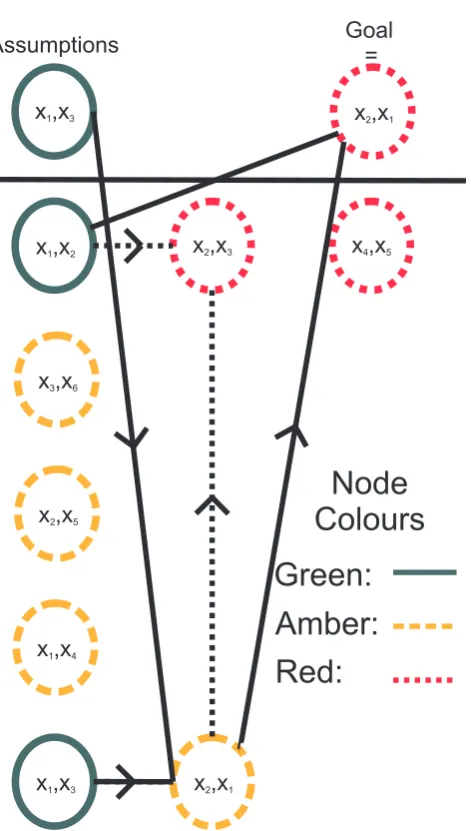
3.1 An activation graph for the Rule 30

reduction described in the previous section. The solid black edges represent a possible activation chain. Green nodes represent equalities, amber nodes represent inequalities and red nodes are not active. The goal is

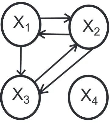
c52,x2 ≤ x1and the assumption isx1 =x3. . . 25 3.2 An inequality graph for the application of Rule 2 to remove

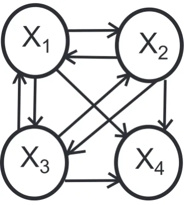
x3 ≤x4fromx1x2x3 ≤lex x2x3x4in the context ofx1x2x3 ≤lex x3x4x1. 27 3.3 Transitive closure of the inequality graph for a CSP with X =

{_x₁,_x₂,_x₃,_x₄}_,C={_x₁ =_x₂,_x₁ =_x₃,_x₂ =_x₃,_x₂_x₃ ≤_lex _x₄_x₁}_. _{. . . .} ₂₈

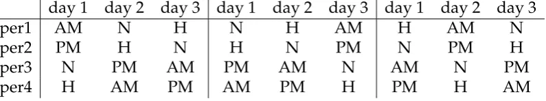
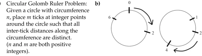
4.1 Three symmetric schedules for the personnel scheduling prob-lem instance, where days=3, people=4, shifts={_AM,_PM,_H,_N}_. ₃₅ 4.2 Specification of the Circular Golomb Ruler problem. Symmetric

solutions to the length 7, 3-tick Circular Golomb Ruler problem. 37

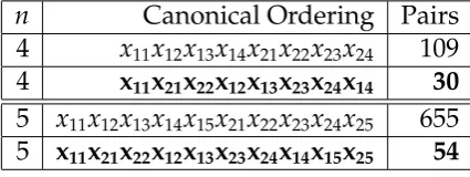
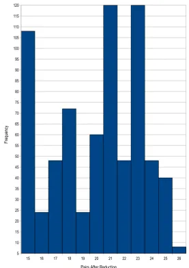
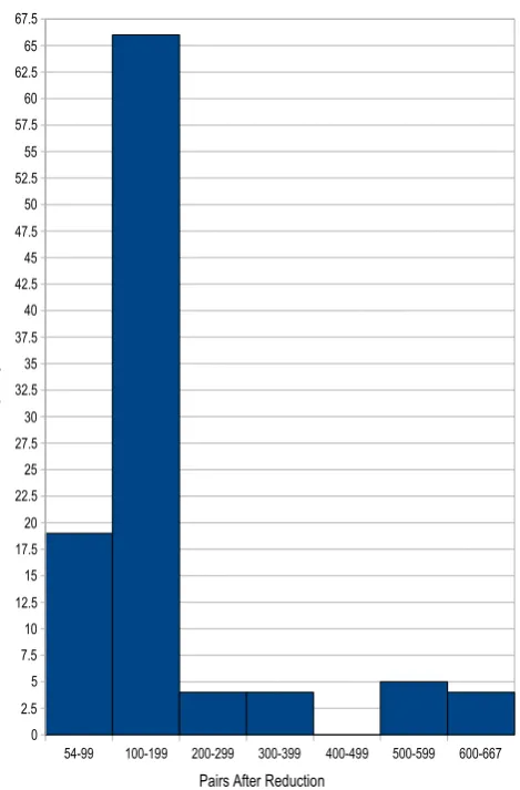
5.1 Results of the reduction of lex constraints for a 2×_n_{matrix . . .} ₅₉ 5.2 Distribution of pairs remaining after reduction for a 2×_{3 matrix}

on all orderings. . . 60 5.3 Distribution of pairs remaining after reduction for a 2×_{4 matrix}

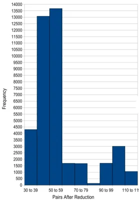
on all orderings. . . 61 5.4 Distribution of pairs remaining after reductions for a 2×_{5 matrix}

(15)

LIST OF FIGURES

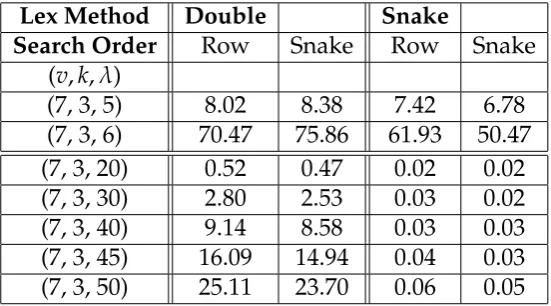
5.6 A comparison of search times, in seconds, on the BIBD problem. The searches above the double line are for all solutions, whilst those under are for one solution. . . 69 5.7 A comparison of search times, in seconds, on the EFPD problem.

In each case there are no solutions. . . 70 5.8 A comparison of search times, in seconds, on the FLECC

prob-lem. The test case above the double line searches for a single solution, whilst those under search for all solutions. . . 71 5.9 A comparison of search times, in seconds, on insoluble instances

of the Howell design problem. . . 72

8.1 This gives the reduction described in Method 1 of Theorem8.2.1. The solid black edges represent a possible activation chain, with the dashed edges representing activations not used in that acti-vation chain. Green nodes are equal, amber nodes are less than or equal and red nodes are not active. The goal is c52, x2 ≤ x1 and the assumption isx1 =x3. . . 102 8.2 This gives the reduction described in Method 2 of Theorem8.2.1.

The solid black edges represent a possible activation chain, with the dashed edges representing activations not used in that acti-vation chain. Green nodes are equal, amber nodes are less than or equal and red nodes are not active. The goal is c62, x2 ≤ x1 and the assumption isx1 =x3. . . 103 8.3 Running D on lex leaders derived from the first 15 transitive

groups on 6 points inGAP’s library. . . 111 8.4 Results from runningDon 10 lex leaders derived from primitive

(16)

Chapter 1 Introduction

Constraints are found extensively in everyday life: how much food should I eat for lunch; how long can I spend in the gym today; how much fuel will it take for my car to travel 80 miles; how much money is in my bank account. It therefore follows that constraint programming is a natural way of explaining many of the problems we encounter. We can model problems as constraint satisfaction

problemsand solve them. This solving process involves assigning potential

val-ues to the variables in a problem and testing whether these assignments satisfy the constraints. Much work has been carried out in the field of CSPs in order to improve the time taken to find a satisfying set of assignments. These include search methods, reformulation of the problem, search heuristics, propagation algorithms, and symmetry breaking. This thesis focuses on symmetry breaking as a method to improve search in CSPs.

(17)

1.1 Topic of this Thesis

by remembering which paths the search process has taken and ensuring that no symmetric paths are followed at a later time. This thesis focuses on static symmetry breaking.

The most famous static symmetry breaking technique, proposed by

Craw-fordet al., is the lex-leader method. The lex leader method posts lexicographic

ordering constraints to the CSP model in order to search for just one member of each equivalence class. This method can produce a huge number of constraints and as such a number of rules for the reduction of these constraints have been developed. The reduced constraints maintain the reduced search tree provided by the complete lex constraints, but require a smaller memory footprint and generally utilise fewer propagators during search. This thesis picks up the research in this area from this point. We describe the theoretical processes nec-essary to produce a minimal set of lex constraints which are required to break all of the symmetry in a CSP model automatically.

1.1 Topic of this Thesis

Statically breaking variable symmetries by adding lexicographic ordering con-straints is widely used and implemented [10][24][22][6]. Two issues arise when using this method: the number of constraints required can be exponential and therefore be prohibitively costly when used to help solve CSPs[19][46][24]; util-ising such symmetry breaking techniques requires expertise in the subject area as well as a great deal of time and effort[47].

(18)

1.2 Aims

1.2 Aims

The aims of this thesis are to:

• _{investigate methods of reducing the size and arity of lex constraints.}

• _{describe the operation of lex reduction rules in a manner suitable for}

examining their operation – in particular their temporal nature.

• _{reduce lex constraints for members of commonly-occurring families of}

groups.

• _{generalise the group reductions so that we have formulae for producing}

minimal constraints for any member of the commonly-occurring infinite families of groups.

• _{investigate di}ff_{erent canonical orderings of lex constraints w.r.t. matrix}

row and column symmetries.

• _{define an incomplete symmetry breaking method that can outperform}

known incomplete methods for breaking row and column symmetries.

• _{investigate methods to compose symmetry breaking constraints for direct}

products and imprimitive wreath products.

• _{provide an introduction to the use of}_GAP_{for manipulating permutation} groups.

• _{describe an algorithm to decompose a group into products of groups for}

which a general formula has been described so that a small set of lex constraints can be produced automatically.

• _{investigate whether the order of application of the lex reduction rules}

affects the minimal set of constraints achieved with a view to proving that the formulae for producing minimal constraints actually produces minimum constraints.

(19)

1.3 Summary of Contributions

1.3 Summary of Contributions

The main aim of this thesis is to provide a method of automatically generating minimal ordering constraints to break variable symmetries in constraint sat-isfaction problems. In order to achieve this several other contributions have been established:

• _{Two graph-based representations of the operation of the reduction rules}

for lexicographic ordering constraints. One, an activation graph, pro-vides a temporal view of the progression of the reduction as well as providing an understanding of which variables provide support for the removal of another by introducing the concept of an activation chain. The second representation, an inequality graph, describes how an algorithm to implement the reduction works computationally.

• _{Four general formulae for the production of minimal ordering constraints}

for some commonly-occurring infinite families of symmetries in CSPs. These general formulae, with respect to the number of variables in the CSP, can produce minimal sets of lex constraints in a linear time and are linear in size.

• _{An investigation into the e}ff_{ects of di}ff_{ering canonical variable orders in}

lex constraints to break row and column symmetries w.r.t. the size and arity of constraints left after reduction.

• _{A new incomplete symmetry breaking method, snake lex, for row and}

column symmetries which compares favourably to the current state of the art.

• _{A method of combining minimal symmetry breaking constraints capable}

of breaking symmetries formed from the direct product and imprimitive wreath products of smaller groups.

(20)

1.4 Structure of this Thesis

• _{A context free grammar for describing the symmetries of a CSP as a}

decomposition of the whole symmetry group. This grammar includes sufficient data to maintain the mappings between points and variables. This mapping information is necessary to help produce lex constraints that break the symmetries.

• _{A program to decompose a symmetry group into products of smaller}

groups. This code can only deal with the groups and products discussed later on in this thesis. Provision has however been made for allowing extensions to this code at a future date by returning generators for any undescribed group.

• _{A proof that the reduction of lex constraints by the reduction rules is not}

in general confluent.

• _{A proof that the formulae for the production of minimal lex constraints for}

some infinite families of symmetries produce the minimum constraints.

• _{A definition of a}_block_{that characterises the areas of a set of lex constraints}

where a choice of reduction paths with distinct roots occur.

• _{The introduction of an algorithm to decide whether a set of lex constraints}

will reduce confluently, and hence will always reduce to the optimal set of constraints.

1.4 Structure of this Thesis

(21)

1.4 Structure of this Thesis

(22)

Chapter 2 Background

2.1 Constraint Satisfaction Problems

Constraint Satisfaction Problems (CSPs) involve enforcing local constraints on values that can be assigned to variables in order to solve a problem. The field began to appear around the time of the publication of Alan Mackworth’s machine vision paper [38] and also Ugo Montanari’s picture processing pub-lication [44]. The representation of CSPs consists of a number of variables, a domain of values for each variable, and a set constraints over the variables. These constraints define allowed combinations of values over a subset of the variables.

Definition 2.1.1. A CSPAis a tripleA= hX,D,Ci_whereX_{is a set of n variables} X= {_x₁_,x₂_,. . ._,x_n}_,D_{is a corresponding set of n domains, which are sets of values,}D

= {_d₁_,d₂_,. . ._,d_n}_{such that x}_i ∈ _d_i _,and C_{is a set of constraints}C= {_c₁,_c₂, . . . ,_c_t}_{. A}

constraint cj is a relation over a subset ofX.

When trying to find a solution, a complete assignment of values to vari-ables such that all constraints are satisfied, we employ two major classes of techniques,propagationandsearch.

(23)

2.1 Constraint Satisfaction Problems

representing the relation x1 < x2. We can clearly see that 3 can never be assigned tox1in any solution, and likewise 1 can never be assigned tox2in any solution. We therefore remove these values from their respective domains. A problem in which no values can be removed from any domain is described as

consistent.

Search involves assigning values to variables and testing if complete as-signments are solutions or if partial asas-signments can be extended to solutions;

partial solutions.

2.1.1 Consistency in Constraint Satisfaction Problems

There are a number of different levels of consistency in CSPs. The simplest of these isnode-consistency. Node-consistency ensures that all unary constraints, those relating to just one variable, hold for every value in that variable’s do-main. Enforcing unary consistency is a trivial process.

A variable xi is arc-consistent with another variable xj if, for every value dk ∈Dithere exists a valuedl ∈Djsuch that (dk,dl) satisfies the binary constraint

betweenxiandxj. A problem is arc consistent if every variable is arc consistent

with every other one [39] [40] [3] [57].

Path-consistencyis similar to arc-consistency but considers pairs of variables

instead of only one. A pair of variables is path- consistent with a third variable if each consistent assignment of values to the pair can be extended to the other variable such that all binary constraints are satisfied. xi and xj are path

consistent withxk if,xi and xj are arc-consistent, and for alldl ∈ Di and for all dm ∈ Dj there exists a value dn ∈ Dk such that (dl,dn) and (dm,dn) satisfy the

constraint betweenxi andxkand betweenxjandxk [39] [44].

(24)

2.1 Constraint Satisfaction Problems

2.1.2 Search in Constraint Satisfaction Problems

The simplest complete method of searching for a solution to a CSP is to generate every possible assignment of values to variables and test to see if all constraints hold with these assignments. We call this methodgenerate and test. This method is trivially both complete and correct, but it is of course very inefficient. A simple improvement to this algorithm ischronological backtracking[4].

Backtracking involves checking for consistency after each value assignment to a variable. If any domain becomes empty during this process, we undo the assignment of the value to the last variable and continue at the next value in the domain. In selecting the next value to assign we can simply work through our domains in order, however very good results have been obtained by dy-namically selecting the next value and variable assignment after backtracking [43].

There exist stochastic search methods for CSPs [52]. These generally begin with a random assignment of values to variables then attempt to find a solution by searching from this initial seed point. This can be an effective method of searching for solutions, particularly when the search space is very large. However there are a number of limitations to this approach. The search method is incomplete, therefore you can never prove that there are no solutions to a problem. If you do find a solution, you have no way of knowing if it is the best solution and furthermore you cannot enumerate all solutions. Another feature of this search technique is that it does not operate well with symmetry breaking constraints since the process may be searching in areas of the search tree that the symmetry breaking constraints have removed all of the solutions from. In some cases, adding more symmetry to the problem reduces the solve time [48]. We therefore only use backtracking based algorithms in this thesis.

2.1.3 Global Constraints

The arity of a constraint is the size of the scope of that constraint. Unary

constraints are relations on single variables. For example, x1 , 6 is a unary

(25)

2.2 Symmetries

terms of unary and binary constraints since many of the useful propagation and search algorithms have this as a requirement. It is however possible to have k-ary constraints, 3 ≤ _k ≤ _n_{, but it is also possible to restate any} _k_-ary constraint as a set of binary constraints.

Sometimes it is useful to leave k-ary constraints as they are, particularly when dealing with a set of constraints called global constraints. These are relations over a number of variables, which occur often. Specific methods of propagation exist to facilitate search in these cases. The most notable and widely used global constraint isalldifferent.

Definition 2.1.2. Let x1,x2, . . . ,xnbe variables. Then

alldifferent(x1,x2, . . . ,xn)={(d1, . . . ,dn)|∀idi ∈D(xi),∀i,jdi ,dj}[35]

Puget proposed using a set of less than constraints over the variables and using a specialised propagation algorithm; the highest and lowest values of each domain are members of a consistent problem. [49] Improvements over this algorithm were proposed by Lopez-Ortizet al. [36]

2.2 Symmetries

One important area of research within the field of constraint programming is that of symmetries. Symmetries are interesting because they represent branches of a search tree which are essentially repeats of a previous branch or branches. If we can detect and then remove these symmetries then the resulting search tree has fewer nodes, and therefore, in theory, can be computed more efficiently provided that the overhead in breaking the symmetries is not too large.

2.2.1 Computational Group Theory

(26)

2.2 Symmetries

id x11 x12 ρ x12 x11

x21 x22 x22 x21

θ x21 x22 ρθ x22 x21

x11 x12 x12 x11

The top left matrix is the standard order that we would generally use to describe a matrix, we call this the identity. The permutation ρ swaps the columns, andθswaps the rows. We can combine the permutationsρandθto produceρθwhich swaps both the rows and the columns. If we now map the four variables{_x₁₁,_x₁₂,_x₂₁,_x₂₂}_{onto the points}{1,2,3,₄}_{we can view these four} permutations inCauchyform.

id 1234₁₂₃₄ ρ 1234

2143

θ 1234 3412

ρθ 1234 4321

The top line of each permutation is the canonical form, the bottom line is the permutation of the points described byρ,θ, andρθ. It is more common to describe permutations in cycle form.

id () ρ (12)(34)

θ (13)(24) ρθ (14)(23)

Takingρabove as an example, this cycle describes a permutation where 1 maps to 2 and 2 maps to 1. Also, 3 maps to 4 and 4 maps to 3. As you can see from the identity, mappings of variables to themselves are ignored.

Now that we have an understanding of permutations we extend this knowl-edge to the formal definition of apermutation group.

Definition 2.2.1. Group Axioms

A permutation group is a non-empty setPwith a composition operator·_{such that:}

-Pis closed under·_{. That is for all g},_h∈P_{, g}·_h∈P_;

(27)

2.2 Symmetries

-every element g ∈P_{has an inverse g}−₁

such that g· _g−₁₌

g−₁_·

g=id;

-·_{is associative. That is, for all f},_g,_h∈ P_,₍_f · _g₎·_h= _f ·₍_g·_h₎_.

The inverse of ρ in the matrix example above is itself, therefore ρρ = id. The set of permutations are also clearly associative since ρθ = θρ. We can compose any number of the permutations given for the matrix symmetries, but the group only contains four permutations. This is because the composition of some permutations produce already known permutations. For example, ρθρ =θ. We call the number of permutations in a group itsorder, or size.

Definition 2.2.2. Order of a group

The order of a groupPis the number of elements in the group. It is denoted|P|_.

Since we can compose permutations to create different permutations, there exists a set of permutations that we can compose to form the entire group. We call such a set thegeneratorsof the group.

Definition 2.2.3. Generators of a group

LetSbe any set of permutations that can be composed by the group operation·_{. The set}

SgeneratesPif every permutation ofPcan be written as a product of permutations in

Sand every product of any sequence of permutations ofSis inP. The setSis called a

set of generators forPand we writeP=hSi_.

A subset of the permutations inPis not necessarily enough to produce the entire set of permutations in P. A set of permutations which are inP but are not capable of being used to compose all of the permutations inPcan be used to form a subgroup ofP.

Definition 2.2.4. Subgroup

A subgroup H of a group P is a subset of P that is itself a group with the same

composition operator asP. Pis a subgroup ofP, as is{_id}_.

(28)

2.2 Symmetries

the point δ to another point using the permutation g. One can imagine a 3×_{3 matrix with rotational symmetry. Where this symmetry to be represented} group theoretically, the orbit of the top left hand cell is the set of all 4 corners whereas the orbit of the central cell is only itself.

Definition 2.2.5. Orbit

The orbit of a pointδinPis the setδP ={δg_|_g_∈ _P_}_.

A group istransitiveif every point can map to every other. Transitive groups only have one orbit, the set of all points. Intransitive groups have more than one orbit. The group which fixes a point such that it only maps to itself is called astabiliser.

Definition 2.2.6. Stabiliser

Let Pbe a permutation group acting on a pointβ. The stabiliser ofβ inPis defined

by: Pβ ={g∈P|βg =β}. The stabiliserPβis a subgroup ofP.

Examples of some families of groups are described in chapter4.

2.2.2 Variable Symmetries in CSPs

Symmetries are defined in a number of ways, some of which portray the same fundamental principles and others which are fundamentally different. Two definitions of symmetry exist in CSPs: solution symmetry; andproblem symmetry. A solution symmetry is a permutation of d-values that preserves the set of solutions. It is a bijective mapping from one set of solutions to another set of solutions.

Definition 2.2.7. Solution Symmetry

A solution symmetry of a CSPAis a symmetry ofAfor sols(A), i.e. a permutationρ

of d-vals such that sols(A)ρ=sols(A).

(29)

2.2 Symmetries

Definition 2.2.8. Microstructure

For any binary CSP instanceA =hX,D,Ci_{, the microstructure of}A_{is a graph with}

set of verticesX×D_{where each edge corresponds either to an assignment allowed by a}

specific constraint, or to an assignment allowed because there is no constraint between the associated variables.

An automorphism of the microstructure is a bijective mapping of the ver-tices of the graph which preserves the edges. Any automorphism of the mi-crostructure must be a problem symmetry of the CSP.

Definition 2.2.9. Problem Symmetry

For any binary CSP instance A = hX,D,Ci_{, a constraint symmetry is an}

automor-phism of the microstructure ofA.

These definitions were introduced and discussed extensively by Cohenet al. [7]. Two interesting symmetries which are special cases of the two defined above arevalue symmetriesandvariable symmetries.

Definition 2.2.10. Value Symmetry

Avalue symmetryof a CSP is a bijection f : Di → Di, for1≤ i≤ |D|, of the set of values such that{h_x_i,_d_ii _{: 1}≤_i≤_n}_{is a solution if and only if}{h_x_i, _f₍_d_i₎i _{: 1}≤_i≤_n}

is a solution.

Definition 2.2.11. Variable Symmetry

Avariable symmetryof a CSP is a bijection f : X→ X_{of the set of variables such}

that {h_x_i,_d_ii _{: 1} ≤ _i ≤ _n}_{is a solution if and only if} {h_f₍_x_i),_d_ii _{: 1} ≤ _i ≤ _n}_{is a}

solution.

Consider the problem X = {_x₁,_x₂}_, _d₁ = {1,2,₃} _d₂ = {1,2,₃}_{, and a single} constraint representing the relationx1 ,x2. Clearly we can see thatx1 =1 and

x2 =2 is a solution, but by swapping the variables we can also get the solution

x2 =1 andx1=2. We call the later solution a symmetry of the first. Symmetric solutions are grouped into sets called equivalence classes. Equivalence classes relate to the orbits of the symmetry group.

(30)

2.3 Symmetry Detection

2.3 Symmetry Detection

In order to utilise symmetries in CSPs we need to detect their existence. Tradi-tionally this has been done by hand, a process which is both time consuming and generally produces an incomplete set of symmetries. Much work has been directed towards automating the process of detecting symmetries.

We can remodel a CSP as a graph. Puget offers an automated detection method for variable symmetries using graph automorphism.

Definition 2.3.1. Given a coloured graph G = hV_,E_,ci_{, where} V _{is a finite set of}

vertices,Eis a set of edges between these vertices and c is a function fromVto integers,

an automorphism of G is a bijection f fromVtoVsuch that:

∀_e∈E, _f₍_e₎∈E

∀_v ∈V, _c₍_f₍_v₎₎=_c₍_v₎

[50]

Although this has shown some success the problem of graph automorphism is in the class of problems NP, and as such its scalability is questionable. [53] Various tools are however available to assist in this process, NAUTY [41], SAUCY [11] and AUTOM [50].

Another point of interest raised by Frischet al. [18] is that symmetries can be introduced by decisions made during the modelling process. If we can identify which symmetry groups are added, and when, then we can automate the addition of symmetry breaking constraints to a model.

(31)

2.4 Symmetry Breaking

2.4 Symmetry Breaking

Having identified a symmetry group within a CSP it then remains to utilise the symmetry. We call this utilisation symmetry breaking. The objective of symmetry breaking techniques is to leave one member of each equivalence class of assignments, or a subset of these assignments in the case of some specific techniques. This can be achieved in two main ways: static symmetry

breaking; anddynamic symmetry breaking.

2.4.1 Dynamic Symmetry Breaking

Dynamic symmetry breaking methods alter the search process such that once an assignment has been discarded, no symmetric assignment will be explored. They do this by remembering which paths the search process has taken and ensures that no symmetric paths are followed at a later time.

The first major dynamic symmetry breaking algorithm wasSymmetry

Break-ing DurBreak-ing Search[2] [21]. It imposes constraints at each node where a failure

has been detected that ensures that no symmetric failures are searched over. A major issue with this is that when symmetry groups are very large, an expo-nential number of constraints may be added to the problem.

The next step in dynamic symmetry breaking was the advent of the sym-metry breaking by dominance detection algorithm [13] [15]. With this method we only search down the dominant nodes.

Definition 2.4.1. No-good

Node v in a search tree is a no-good w.r.t. n if there exists an ancestor naof n such that

v is the left hand child of na and v is not an ancestor of n.

Definition 2.4.2. Dominance

A node n is dominated if there exists a no-good v w.r.t. n and a symmetry g such that

(δ(v))g_⊆_∆₍_n₎_{. v dominates n.}

(32)

costly. Computational group theory has gone someway towards remedying this situation. GAP-SBDD [20] is one such method that has proven useful in practice.

2.4.2 Static Symmetry Breaking

Static symmetry breaking involves adding constraints to the model before search in order to reduce the number of (non-)solutions in each equivalence class, usually to one.

The most famous of static symmetry breaking techniques, proposed by Crawfordet al., is the lex-leader method [10] [37].

We first define a canonical ordering on the decision variables, then add one constraint per symmetry that orders the assignments to these variables. To illustrate, we consider the symmetric groupS3acting on variables{x1,x2,x3}.

{(),₍_x₁,_x₂),₍_x₂,_x₃),₍_x₁,_x₃),₍_x₁,_x₃,_x₂),₍_x₁,_x₂,_x₃₎}

We choose x1 to be the most significant variable in the ordering, x2 the next most significant, and x3 the least significant. The next step is to add

lexico-graphic ordering constraints (lex constraints) to allow only one member of each

equivalence class of assignments induced by the symmetry.

x1x2x3≤lex x2x1x3, x1x2x3≤lex x1x3x2, x1x2x3 ≤lex x3x2x1

x1x2x3 ≤lex x2x3x1, x1x2x3 ≤lexx3x1x2

Notice that there is one constraint per nontrivial permutation ofS3. In general, there aren! permutations for the groupSnand so (n!−1)n-ary constraints are

produced by the lex-leader method to break all symmetries. A more in depth look at lex constraints can be found in chapter3.

(33)

(34)

Chapter 3 Reduction Rules

3.1 Introduction

This chapter introduces lexicographic ordering constraints (lex constraints) and discusses ways to improve the efficiency of their application. Much of this chapter has appeared in previous peer-reviewed publications by the author of this thesis [24][25][23][27][26]. We begin by describing graph based methods to clarify the process involved in working with lex constraints. Sections 3.2 and 3.3 introduce two views of lex constraints. The former is a view useful for the human understanding of their function, whilst the later is closer to computerised method of dealing with the constraints. These views will be used extensively throughout chapters4,6, and7.

Lex constraints are an effective method to break symmetries in some CSPs. The disadvantage of this method however is that, for a CSP with n = |X|_{, it} produces up to n! lexicographic ordering constraints, each with arity n. The overhead of adding this number of constraints to the CSP usually outweighs the benefit of breaking the symmetry.

(35)

3.1 Introduction

δdenote strings of variables, Rules 1, 2 and 3 are stated:

1 Given a constraintcof the formαxiβ≤lex γxjδ, ifα=γentailsxi =xj then

replace it withαβ≤_lex γδ.

2 IfCis a set of constraints of the formC0_{∪ {}_α

xi ≤lex γxj}, andC0 ∪ {α=γ}

entailsxi ≤xj, then replaceCwithC 0_{∪ {}

α≤_lex γ}_.

3 IfCis a set of constraints of the formC0_{∪ {}_α

xiβ ≤lex γxjδ}, andC0∪ {α=γ}

entailsxi =xj(orxi ≤xjwhen|β|=0), then replaceCwithC0∪{αβ≤lex γδ}.

Rule 3 extends Rules 1 and 2 in that it allows both the consideration of all pairs of variables in any one lex constraint, provided by Rule 1, and the impli-cations derived from considering the entire set of lex constraints, provided by Rule 2. Unfortunately the support required for removal of the least significant pair remains essentially different from that required for the removal of any other pair. Whilst Rule 2 requires the condition of inequality in order to prune variable pairs from lex constraints, Rule 3 generally requires equality. Talking solely about Rule 3 during theorem proving is tedious since we must always include the clause,except when examining the least significant pair. For this reason we find it useful to remove the action of ¨Ohrman’s Rule 3 that covers the actions of Rule 2 and to restate it as Rule 30

. Furthermore, the application of Rule 1 is a relatively lightweight process and it is therefore sensible to still consider Rule 1, even though it is still superceded by Rule 30

. The three rules we use in this chapter, and from now on, are defined below.

Definition 3.1.1. Lettingα, β, γ,andδdenote strings of variables, we define Rules1,

2and30 .

1 Given a constraint c of the form αxiβ ≤lex γxjδ, if α = γ entails xi = xj then

replace it withαβ≤_lex γδ_.

2 If C is a set of constraints of the form C0 _{∪ {}_α

xi ≤lex γxj}, and C0 ∪ {α = γ}

entails i≤ _{j, then replace C with C}0_{∪ {}_α_≤

lex γ}.

30 If C is a set of constraints of the form C0 ∪ {α_x_iβ ≤_lex γ_x_jδ}_{, and C}0 ∪ {α= γ}

entails xx =xy, then replace C with C

0_{∪ {}_αβ_≤

(36)

Correctness for these rules was shown by Frisch and Harvey [19] and ¨

Ohrman [46].

As an example of Rule 1, consider a constraintc: x1x2 ≤lex x2x1. To ensure thatcis satisfied we need only compare a pair of variables if each pair of more significant variables are equal. Ifx1 = x2then trivially the second pairmustbe equal. Therefore, by Rule 1 we need only consider the first pair of variables, reducingctox1 ≤x2without modifying the set of solutions.

For Rule 2 we can also use the rest of the constraints to justify the removal of our pair under consideration. Consider the two constraints c1 = x1x2x4 ≤lex

x2x3x5andc2 =x1x4 ≤x3x5where we are attempting to remove the pairx4 ≤x5

from constraintc1. We first assumex1 =x2andx2 =x3since the least significant pair in this constraint will only be considered if all more significant pairs are equal. Using these assumptions we can see that the first pairc2becomesx1 =x3 . This means that when we get to the stage wherex4≤x5is actively being used

inc1,x4 ≤x5is also constraining the same variables inc2. We can therefore say thatx4 ≤x5inc1is entailed and it can be removed by Rule 2.

For an example of the way in which Rule 30

operates, we consider TransitiveGroup(6,6)inGAP’s library [9,56]. The group elements are:

(), (36), (153)(264), (153426), (14)(36), (132465), (25)(36), (156423), (135)(246)

(156)(234), (135462), (132)(465), (14), (126453), (126)(345), (162435),(25), (165)(243), (14)(25), (162)(354),(165432),

(123)(456), (123456), (14)(25)(36)

The group contains 24 elements which we use to construct lex constraints with the canonical ordering, [x1,x2,x3,x4,x5,x6]. Using Rules 1, 2 and 30we partially reduce the full set of lex constraints to:

(1)x1x2x4 ≤lex x2x3x5, (2)x3 ≤lex x6, (3)x2 ≤lex x5, (4)x1 ≤lex x4,

(37)

Suppose we want to apply Rule 30

to the pair x2 ≤ x1 in constraint (5); we assume x1 = x3, since this is the more significant pair in constraint (5), then constraint(6) givesx2 ≤x1because its most significant pair is now equal. Since constraint (1) states x1 ≤ x2, we deduce x1 = x2, and remove x2 ≤ x1 from constraint (5) by Rule 30

. We then have the following set of constraints which is a fixpoint.

(1)x1x2x4 ≤lex x2x3x5, (2)x3 ≤lex x6, (3)x2 ≤lex x5, (4)x1 ≤lex x4, (5)x1x4x5≤lex x3x6x4, (6)x1x2 ≤lex x3x1 .

The reduction rules are applied, in the order, Rule 1, Rule 2 then Rule 30 until a fixpoint is reached. For the remainder of this thesis we utilise Rule 1 as a pre-processing step to further reduction. On the remaining constraints we will use Rule 2 and 30

for reduction to a fixpoint.

Definition 3.1.2. A reachable fixpoint for a setCof lex constraints is a reduced set of

lex constraints produced by removing pairs fromCusing Rules2and30

such that no

further applications of Rules2and30

are possible.

Before continuing with by describing the two viewpoints of the reduction rules, we first prove a lower bound on the number of constraints required to break all permutations of a transitive group acting on variables.

Theorem 3.1.1. Let X = {_x

1,x2, ...,xn} be the set of decision variables of a CSP P. Assume that P has a transitive group of variable symmetries and that each domain has

size at least2. Then, not considering any other constraints in P, the minimum number

of binary≤_{constraints required to remove all but one member of each equivalence class}

of assignments is n−₁_.

Proof. Any constraint graph withn−_{2 binary constraints is disconnected. Let}

x1 be the most significant variable. Let xi be a decision variable that is not

connected to x1, and such that xi is most significant in its component of the

constraint graph. Letabe the minimal element of the domain ofxi (and hence

of all variables, by transitivity). Let A be any full assignment which assigns

(38)

3.2 Activation Graphs

mapping xi to x1 there is a symmetry mapping A to a full assignment with

x1 = a. Thus there will remain more than one solution from an equivalence class after addition of the n−_{2 binary constraints, and therefore}_n−_{2 binary} constraints will not suffice. Puget [51] has described a set of binary≤_constraints of sizen−_{1 that break all symmetries in some cases. The minimum number is} thereforen−_1.

3.2 Activation Graphs

In order to show if there exists more than one distinct fixpoint when reducing lex constraints using the reduction rules we require a precise understanding of which constraints, and pairs within those constraints, are used by Rules 2 and 30

to remove a pair. This precision is achieved by introducing the notion of an

activation graph. For the remainder of this chapter, letC= {_c₁, . . . ,_c_k}_{be a set of}

lex constraints, not necessarily derived from a group. The pair of variables in position jof constraintiis denotedci j.

Definition 3.2.1. Agoalc_αβis a pair under consideration for removal by Rules2and

30

. Each goal defines an activation graph. An activation graph G_αβis a digraph which

is generated from the assumptions made to remove the goal c_αβ by Rule2or30

.

Thenodes of Gαβ are {ci j |ci ∈ C, j ≤ βif i = α,1 ≤ j ≤ |ci|if i , α}, and are

arranged in k rows, one for each constraint. The nodes are also arranged in columns

from most significant to least significant. The first row is cα, truncated immediately

after cαβ. The order of the other rows does not matter, and they should be considered as

a set.

Non-goal nodes can beactiveorinactive. A node ci jisactiveif i= αand j < β,

or j = 1(the most significant pair), or there is an edge from ci(j−₁₎ to c_{i j}. An active

node ci j is green if the pair of variables are equal, and isamber otherwise. Inactive

nodes arered. The colour of a node may change from red to amber to green, as edges

are added, but not in the other direction. When initially constructing the graph the

(39)

3.3 Inequality Graphs

Let ci j , cαβ, and assume that ci(j−₁₎ is active. A justification setfor c_{i j} is a set of nodes Ai j ={cst|(cst,ci j) ∈ E(Gαβ)}such that if Ai jis nonempty then it entails the equality of ci(j−₁₎. The justification set A_{i j} isminimalif for all x∈ A_{i j}the set A_{i j}−x is insufficient to activate ci j.

There are several types of edges in Gαβ:

1. If ci j , cαβ then there is a directed edge from an active node cstto ci j whenever

there exists a minimal justification set for ci jcontaining cst. If so, there is an edge

from ci(j−₁₎ to c_{i j}, c_i₍_j−₁₎is green, and c_{i j}is amber or green.

2. There is a directed edge from an active node ci j to cαβ when ci jis a member of a

minimal set of nodes entailing c_αβ (Rule2) or entailing equality in the variables

in c_αβ(Rule30 ).

3. There are directed edges between consecutive nodes in row1, from more

signifi-cant to less signifisignifi-cant, up to but not including c_αβ.

The node cαβ can be removed by Rules 2 and 30 if and only if there is a

directed edge intocαβ inGαβ.

Definition 3.2.2. An activation chain for cαβ is a subgraph of Gαβ whose nodes

include cαβand which contains a minimum justification set for each of its nodes. Note

that c_αβcan have more than one activation chain.

Intuitively, an activation chain represents one argument for the removal of cαβ. To clarify these concepts, we present the activation graph G52 for the set {(1), . . . ,₍₆₎} _{of constraints given in the previous section in Figure} _3.1. This is a Rule 30

reduction of a set of lex constraints to break the symmetry TransitiveGroup(6,6).

The concept of reducing to fixpoints and the application of activation graphs is developed further in Chapter8.

3.3 Inequality Graphs

(40)

Green:

Amber:

Red:

Node

Colours

x ,x1 3

x x2, 3

x x3, 6

x x2, 1

x x1, 2

x x2, 5

x x1, 4

x x1, 3 x x2, 1

Assumptions Goal₌

[image:40.595.196.432.183.599.2]

x x4, 5

Figure 3.1: An activation graph for the Rule 30

(41)

process of applying each rule. Another useful way of visualising the reduction rules is in the form of a directed graph. The nodes of this graph are the variables in the CSP, and the edges represent inequalities between them. We call these graphsinequality graphs. Inequality graphs are a much lower level description of the operation of the reduction rules and are closer to the computational representation than that of an activation graph. Inequality graphs describe one possible way to implement the reduction rules.

Definition 3.3.1. Given a CSP A = (X,D,C), the corresponding inequality graph

G = (X,E)is a directed graph with one node per element ofX. G contains the set of

directed edges E as follows. If, for some xi,xj ∈ Xand strings of variablesαandβ, C

contains:

1. xi ≤xj then G contains a directed edge from xi to xj.

2. xi =xj then G contains a directed edge from xito xj, and a directed edge from xj

to xi.

3. xiα≤lex xjβthen G contains a directed edge from xi to xj.

Given a set of lexicographic constraints Con variables X, we consider the process of applying Rule 2 to remove the least significant pair of variables in some c ∈ C. Following the rule, we begin by adding equality constraints between all more significant pairs of variables, xi,xj inc. To illustrate, Figure

3.2 shows the inequality graph for a CSP where X = {_x₁,_x₂,_x₃,_x₄}_{, and the} constraints are

(1)x1x2x3≤lex x2x3x4

(2)x1x2x3≤lex x3x4x1

in which x3 ≤ x4 from constraint (6) is under consideration for removal by

Rule 2. The assumed equalities, x1 = x2 andx2 = x3, are represented by dual directed edges between the respective nodes and the inequalityx1 ≤x3entailed byx1x2x3 ≤lex x3x4x1is represented by a directed edge fromx1tox3.

(42)

X

₂

X

₁

X

₄

[image:42.595.218.399.147.350.2]

X

₃

Figure 3.2: An inequality graph for the application of Rule 2 to removex3 ≤x4 fromx1x2x3≤lex x2x3x4in the context ofx1x2x3 ≤lex x3x4x1.

Definition 3.3.2. Consider a directed graph G= (X,E), whereXis the set of nodes

and E is the set of edges. The transitive closure of G is a graph G0 ₌_(X,

E0

)such that

for all xi,xj ∈ Xthere is an edge(xi,xj)in E0 if and only if there is a path from xi to xj in G [45].

Returning to our example, since there is a path fromx3 tox1 viax2, taking the transitive closure of the inequality graph in Figure3.2adds a directed edge from x3 tox1. Since there is now both a directed edge fromx1 tox3, and from

x3 to x1, it is asserted that x1 = x3. This allows us to add the second most significant inequality in the constraint (2), x2 ≤ x4, to the inequality graph. Hence, the inequality graph of this problem now contains a directed edge from

x2tox4. The transitive closure of this graph is shown in Figure3.3. Notice that there is a directed edge fromx3tox4, hence the pairx3andx4 can be removed fromx1x2x3≤lex x2x3x4via Rule 2.

Generally, as described out by Ohrman [46], the operation of establishing the antecedent of Rule 2 can be described as follows:

(43)

X

₂

X

₁

X

₄

[image:43.595.218.398.147.348.2]

X

₃

Figure 3.3: Transitive closure of the inequality graph for a CSP with X = {_x₁,_x₂,_x₃,_x₄}_,C={_x₁ =_x₂,_x₁ =_x₃,_x₂=_x₃,_x₂_x₃ ≤_lex _x₄_x₁}_.

2. Generate the inequality graphGforAand take its transitive closure,G0.

3. IfG0

contains edges corresponding to inequalities not represented explic-itly inA, add these inequalities toAand go to 2.

4. Otherwise, the antecedent of Rule 2 is satisfied if the corresponding edge is present inG0

.

The following lemma characterises the situations in which equality is en-tailed between two decision variables in the context of a CSP containing lexi-cographic ordering and equality constraints.

Lemma 3.3.1. Given a CSP with set of variablesXand set of constraintsC, containing equality and lexicographic ordering constraints, further equality constraints between

pairs of variables xa,xb∈Xare entailed if and only if at least one of the following holds:

1. (transitivity): there exists some xc ∈Xdistinct from xa, xbsuch that xa =xcand

xb=xc; or

(44)

3. there exists some xc ∈ X distinct from xa, xb such that it is entailed that xa ≤

xb≤xcand xc≤xa (and similarly, exchanging the roles of xa, xb).

Proof. Consider an inequality graph,G=(X,E), wherexa,xb,xc ∈X, and where

there exists 0 or 1 directed edges between xa and xb. In order to show that xa = xb we must have a directed edge from xa toxb and a directed edge from xb toxa in Gt, the transitive closure of G. Consider also the graph G0, where

G0 ₌

G− {_x_a,_x_b}_{, in} _G0_t

, the transitive closure of G0

. Adding xa and xb to G0t

with equivalent edges to and fromxa andxb, as inG, leaves a partial transitive

closure graph ofG.

Consider the case wherexa ≤xb, annotated by a directed edge fromxbtoxa.

We can see that inG0_t

if there are only edges fromxaandxbtoG0twe could not

make a path fromxatoxborxbtoxathroughG 0_t

. We can also see that in the case where edges only existed fromG0ttoxa orxbthe same would also be true. We

therefore require at least one edge directed fromxatoG0tand one edge directed

toxbfromG0t.

Wherexa is connected toG0t viaxi andxbis connected fromG0t viaxj there

must also exist some path fromxitoxjto show thatxa =xb. Assume there exists

the node xc in the path from xi toxj, we can then, without loss of generality,

consider a directed edge from xa toxc and a directed edge fromxc toxb. This

represents the inequalityxb ≤ xc ≤ xa. Since we havexa ≤ xb, xa ≤ xb ≤ c and xc ≤xa,xa =xb(similarly where we begin with knowingxb≤xa).

Consider now the case where there is no directed edge betweenxa and xb

or xb and xa. We again require paths fromxa toxb and vice versain much the

same way as in the previous case. Where the two paths are distinct the same reasoning as with the previous example follows: this leaves xa ≤ xb for one

path and xb ≤ xa for the other, thereforexa = xb. Where the two paths follow

the same nodes in opposite directions we can then, again assuming that xc is

on the path, without loss of generality, consider directed edges from xa toxc

and xc toxa, and directed edges fromxc toxb andxb toxc. This represents the

equationsxa =xcandxb=xc, thereforexa =xb.

(45)

Having shown the ways in which equality can be entailed within lex con-straints we now make an observation about the application of Rule 30

.

Corollary 3.3.1. Given a set of lexicographic ordering constraints, a pair of variables, that are not the least significant pair in that particular constraint, can be discarded

using Rule 30

if and only if it is entailed to be equal by Lemma 3.3.1or the pair was

assumed to be equal under the actions of Rule30

.

Additionally we note a relationship between the entailments derived from assumptions over a set of variables and the entailments derived from assump-tions over a subset of these variables.

Corollary 3.3.2. Given a set of lexicographic ordering constraints, L, on the set of variables x1. . .xn, and a set of equality constraints,C, between pairs of variables xi, xj,

a set of equalities, E, are entailed from Lemma3.3.1. Given L andC0, C0 ⊂ C_{, a set of}

inequalities E0

, E0 _⊆

E, are entailed from Lemma3.3.1.

We also establish a useful pattern in the simplification of a set of lexico-graphic ordering constraints.

Lemma 3.3.2. Given a set of lexicographic ordering constraintsC, and some c∈C_of

the form x1. . .xi ≤lex y1. . .yi, the pair xi, yican be discarded from c by Rule2if and only if xi ≤ yi is entailed under the assumptions: x1 = y1, x2 = y2, . . ., xi−₁ = y_i−₁.

This requires xi, or a variable assumed to be equal to xi, to appear on the left-hand side

of some c0 _∈ _C

, where c ,c0.

Proof. Consider an inequality graph, G = (X,E), where xi ∈ X. Consider also

the graphG0

, whereG0 ₌

G− {_x_i}_{, and}_G0_t

, the transitive closure ofG0

. Adding

xitoG0twith equivalent edges to and fromxi, as inG, leaves a partial transitive

closure graph ofG.

Assume first of all thatxi has no edges to any other node in the graph. The

transitive closure of this new graph leavesxi disconnected since no path to or

fromxi can exist, therefore the pair under consideration cannot be removed.

Assume now that there exists directed edges only fromxitoG 0_t

, indicating that xi is less than or equal to some element(s) in G

0

(46)

3.4 Conclusions

appearing on the left hand side of some inequality in C. In this case it is possible that there exists an edge fromxitoyi, and the pair under consideration

could be removed.

The same idea can then be extended to sets of nodes larger than one. Where

xi =xj, there must still exist an edge from eitherxiorxj toG0tin order to show

thatxiis less than another node inG.

3.4 Conclusions

(47)

Chapter 4 Minimal Formulae for Some

Families of Variable Symmetries

4.1 Introduction

The majority of work in this chapter, including all theorems and proofs, has appeared in previous peer-review publications by the author of this thesis [24][25][23].

The rules for the reduction of lexicographic ordering constraints can be an effective way of reducing lex constraints which in turn reducing the solve time of a given CSP However, these reductions come at a cost. Using the transitive closure based algorithm proposed in [46] and discussed in Chapter 3 can be prohibitively costly. The reduction of the lex constraints forS10 is not possible within 24hrs andS13begins to have memory difficulties on a 4Gb machine[24]. Groups of this family and size are very common in CSPs.

In this chapter we aim to eliminate the necessity to use the reduction algo-rithms by describing minimal sets of ordering constraints that can be produced in a time linear in the number of points the symmetry group acts on.

(48)

4.2 Symmetry Groups

groups. In the following sections we then describe a general formula for each group that can be used to create a minimal sound-and-complete set of lex constraints in linear time.

4.2 Symmetry Groups

4.2.1 Symmetric Groups

The symmetric group, Sn, is the group whose elements are the set of bijections

from {1, . . . ,_n} _{into itself, of which there are} _n_{!. Symmetric groups arise} fre-quently as symmetries of CSPs, in particular whenever a set is modelled as a list or an array we introduce the symmetric group on variables. This symmetry is also present when we model a set of sets using set variables.

4.2.2 Example

Consider the following trivial CSP: ({_x

1,x2,x3},di ∈D ={1,2,3,4,5}for 1≤i ≤ n,{_x₁_,_x₂,_x₂_,_x₃,_x₁ _,_x₃}_).

Here we can see that since all of the variables have the same domain, and since each variable has the same constraints over it, that any variable can be interchanged with any other. This CSP has symmetry group S3on variables.

The permutations of this group are as follows.

(),(12),(13),(23),(123),(132)

The lexicographic ordering constraints required to break this symmetry are described below, one for each permutation, in the order they appear above.

x1x2x3 ≤lex x1x2x3

(49)

Running the reduction algorithm on these constraints produces the follow-ing reduced set of lex constraints.

x1 ≤lex x2

x2 ≤lex x3

Section 4.3.1 describes how these constraints could be obtained without running the reduction algorithm.

4.2.3 Cyclic Groups

If all elements of a group C can be written as powers of some fixedρ∈_{C then}

C is cyclic. Just as the name suggests, the cyclic groups describe symmetries

where variables can permute directly with their neighbour on the right, cycling back round to the left for the rightmost variable. Combinations of these per-mutations produce n distinct permutations in a CSP withn variables. In this subsection we detail a problem that exhibits cyclic symmetry, then describe a set of lex constraints for breaking the cyclic group in that problem. Additionally we will describe the minimal set of lex constraints produced upon reduction of the complete set using the reduction rules.

4.2.4 Example

The general personnel scheduling problem is to assign tasks to staff mem-bers while satisfying a variety of different constraints. The following simple example exhibits cyclic symmetry.

Givenn personnel and δdays, for each day, assign each person to one of the shifts{_{AM, PM, Night, Holiday}}_.

Such that:

(50)

day 1 day 2 day 3 day 1 day 2 day 3 day 1 day 2 day 3

per1 AM N H N H AM H AM N

per2 PM H N H N PM N PM H

per3 N PM AM PM AM N AM N PM

[image:50.595.113.511.143.217.2]

per4 H AM PM AM PM H PM H AM

Figure 4.1: Three symmetric schedules for the personnel scheduling problem instance, where days=3, people=4, shifts={_AM,_PM,_H,_N}_.

• _{Shift Pattern: A night shift for a particular person is preceded by either}

an AM shift or a Holiday.

• _{Shift Pattern: A night shift for a particular person is followed by a}

Holiday or a PM shift.

The schedule is to be repeated, so dayδcan be viewed as preceding day 1. For a problem with four people and three days, a set of cyclic symmetric solutions is shown in Figure4.1.

Clearly, we can cycle the days. We cannot however freely interchange them because of the constraints which disallow certain shifts to precede and to come after a night shift. We also can’t reverse the schedule because this would require reversing the night shift constraints.

Part of the symmetry group in the above problem is C3. We can break this symmetry by ordering the per1 row of the problem.

The permutations of C3 are as follows.

(),(123),(132)

The lexicographic ordering constraints required to break this symmetry on the set, X = {_x₁,_x₂,_x₃}_{, are described below, one for each permutation except} the identity, in the order they appear above.

(51)

Running the reduction algorithm on these constraints produces the follow-ing reduced set of lex constraints.

x1 ≤lex x2

x1x2 ≤lex x2x3

Section 4.3.2 describes how these constraints could be obtained without running the reduction algorithm.1

4.2.5 Dihedral Groups

Thedihedral group Dnis the symmetries of a regularn-sided shape, for example

D4is the symmetry group of the square. Let the permutations

a=(1,2, . . . ,n)

and

b=(1,n)(2,n−₁₎. . .₍b_n/2c, d₍_n+3)/2e).

All elements ofDn have a unique decomposition as a product of the formaibj

for 0 ≤ _i ≤ _n−_{1 and 0} ≤ _j ≤ _{1. The set of elements for which} _j =_{0 forms the} cyclic group of ordern, whereas the elementsai_b_{all have order 2.}

4.2.6 Example

Figure 4.2a defines the Circular (or Modular) Golomb Ruler problem. Two solutions to the instance of this problem wherenis 7 andm is 3 are shown in Figure 4.2b. Clearly, these solutions are symmetric: one can be obtained from the other via rotation. Furthermore, we can obtain a third and fourth solution by reflecting in a vertical line the two solutions in the figure. The symmetry group here is D3.

The permutations of D3are as follows.

1_{Although in this example the people in AM are all di}_ff_{erent and we could use Puget’s}

Automated static symmetry breaking in constraint satisfaction problems

Automated Static Symmetry Breaking in

Constraint Satisfaction Problems

Andrew Grayland

School of Computer Science

University of St Andrews

A thesis submitted for the degree of

Doctor of Philosophy

Abstract

Acknowledgements

Publications

Contents

List of Figures

Chapter 1

Introduction

1.1

Topic of this Thesis

1.2

Aims

1.3

Summary of Contributions

1.4

Structure of this Thesis

Chapter 2

Background

2.1

Constraint Satisfaction Problems

2.1.1

Consistency in Constraint Satisfaction Problems

2.1.2

Search in Constraint Satisfaction Problems

2.1.3

Global Constraints

2.2

Symmetries

2.2.1

Computational Group Theory

2.2.2

Variable Symmetries in CSPs

2.3

Symmetry Detection

2.4

Symmetry Breaking

2.4.1

Dynamic Symmetry Breaking

2.4.2

Static Symmetry Breaking

Chapter 3

Reduction Rules

3.1

Introduction

3.2

Activation Graphs

3.3

Inequality Graphs

Green:

Amber:

Red:

Node

Colours

X

2

X

1

X

4

X

3

X

2

X

1

X

4

X

3

3.4

Conclusions

Chapter 4

Minimal Formulae for Some

₂

₁

₄

₃

₂

₁

₄

₃