Effects of layer shift and yarn path variability on mechanical properties of a twill weave composite

C O M P O S I T E M AT E R I A L S Article

Effects of layer shift and yarn path

variability on mechanical properties

of a twill weave composite

MY Matveev, AC Long, LP Brown and IA Jones

Abstract

Experimental and numerical analyses of a woven composite were performed in order to assess the effect of yarn path

and layer shift variability on properties of the composite. Analysis of the geometry of a 12 K carbon fibre 22 twill

weave at the meso- and macro-scales showed the prevalence of the yarn path variations at the macro-scale over the meso-scale variations. Numerical analysis of yarn path variability showed that it is responsible for a Young’s modulus reduction of 0.5% and CoV of 1% which makes this type of variability in the selected reinforcement almost insignificant for an elastic analysis. Finite element analysis of damage propagation in laminates with layer shift showed good agreement with the experiments. Both numerical analysis and experiments showed that layer shift has a strong effect on the shape of the stress–strain curve. In particular, laminates with no layer shift tend to exhibit a kink in the stress–strain curve which was attributed solely to the layer configuration.

Keywords

Textile composites, numerical modelling, mechanical properties, variability

Introduction

Mechanical properties of composites with woven reinforcement directly depend on the type of the reinforcement, its properties and its geometry. A large number of previous numerical studies have been devoted to establishing relationships between the par-ameters of a reinforcement and composite properties using a unit cell approach based on idealisation of the reinforcement geometry.1This approach is capable of predicting the Young’s moduli of the composites with high fidelity providing the numerical model has the cor-rect fibre volume fraction. The unit cell approach is often extended towards damage modelling of woven composites. Examples of such modelling include but not limited to modelling of laminated woven compos-ites under quasi-static tension2,3 and high strain rate compaction,4 composites with braided reinforcement5 and 3D composites.6 However, the conventional unit cell approach cannot predict variability of the mechan-ical properties from sample to sample which is usually associated with variability in the intrinsic properties of constituents7,8and the geometry of reinforcements such as yarn and layer misalignments9 arising from textile

and composite manufacturing. This study focuses only on the effects of variability of textile reinforcement geometry, namely yarn paths and layer shift variability. Yarn path variability has been shown to be respon-sible for variability in manufacturing processes such as forming,10mould filling11and curing.12These numerical studies were based on creating geometric models using statistical models of the reinforcement’s geometry. The statistical models can be as simple as a Taylor expansion of the yarn path as proposed by Endruweit and Long11 or based on specific mathematical concepts of random fields as the Ornstein-Uhlenbeck (OU) sheet used by Skordos and Sutcliffe10 or the Karhunen-Loe`ve series expansion used by Vanaerschot et al.13Using experimen-tal data collected from real reinforcement specimens, e.g. in-plane and out-of-plane average yarn paths and their variability, it is possible to create a stochastic model of

Composites Group, Faculty of Engineering, University of Nottingham, UK

Corresponding author:

MY Matveev, Composites Group, Faculty of Engineering, University of Nottingham, University Park, Nottingham NG7 2RD, UK.

Email: [email protected]

Journal of Composite Materials 0(0) 1–13

!The Author(s) 2016 Reprints and permissions:

the reinforcement geometry in a textile pre-processor as was done, for example, by Vanaerschot et al.14

Variability of the positions of layers relative to each other in a woven composite, often referred to as layer shift, has also been recognised as a source of variability in mechanical properties. An exhaustive numerical study for the case of a plain weave composite with random layer shift was carried out by Woo and Suh.15 The modelling approach was based on Monte Carlo simulations assuming that the distribution of the layer shift is uniform and the positions of the layers are independent. It was shown that the Young’s moduli of regular and out-of-phase stacked laminates are the lower and upper bounds of possible Young’s moduli. The distribution of the modulus was found to be asym-metric for small numbers of layers but tended to be symmetric for large numbers of layers. Coefficients of variation (CoV) of the Young’s modulus were as high as 4.5% for a two-layer composite but less than 1.5% for a composite with 32 layers. Experimental evidence on some of these conclusions was presented by Ito and Chou16 who investigated the effect of layer shift experimentally and showed that the Young’s modulus of a laminate with no layer shift is lower than that of random layer shift laminates. Furthermore, the com-posite with no layer shift exhibited strong non-linearity during the tensile experiments. This can be explained by two factors. The first is the fact that yarns aligned through all the layers do not prevent the yarn straighten-ing in contrast to opposstraighten-ing of yarn straightenstraighten-ing when layers (and yarns) are not aligned. The second is related to occurrence of periodic cracks throughout the laminate which result in the occurrence of weak planes and hence reduction of the Young’s modulus.

This paper aims to combine both experimental and numerical studies of two geometric variabilities: yarn path variability and layer shift variability. This will include multi-scale experimental characterisation of reinforcement geometry in section of Geometry charac-terisation, mechanical testing of laminates with different layer shift in Mechanical testing section and numerical modelling of their behaviour in combination with sto-chastic methods for yarn path modelling in Numerical results section. The results are discussed in Discussion.

Experimental programme

Manufacturing of laminates

A twill weave textile manufactured by Carr Reinforcements (style 38391) was used for the experi-mental studies. The textile consisted of 12 K Grafil 34-700 carbon fibres woven with density of 4.2 picks/ ends per cm and an overall areal density of 660 g/m2.

The textile was used to manufacture six-layer laminates with random layer stacking using a vacuum-assisted resin transfer moulding (RTM) process.17 The layers were placed in a steel tool with a 4 mm cavity and were infused with Prime 20LV epoxy resin mixed with Prime 20 Slow Hardener in ratio 100:26. As a result, three flat composite panels (referred as #1, #2 and #3) with a fibre volume fraction of 55% were manufac-tured, with random layer shift resulting from stacking the layers with no attempt to enforcing alignment. Laminates with no layer shift were manufactured by carefully placing layers on top of each other with respect of their geometry, fixing them in place by metal pins and binding them together with a thermo-plastic NeoXil binder. This procedure should have pre-vented any possible layer shifts during handling and manufacturing of composite panels. Two panels with a layer shift (#4 and #5) with fibre volume fraction of 55% were manufactured using this procedure.

Geometry characterisation

The geometry of the reinforcement was characterised using two techniques:m-CT at the meso-scale (approxi-mately a unit cell size 14 mm) and optical imaging of the textile surface at the macro-scale (>200 mm). The first technique was used to acquire information about the internal structure of the reinforcement which includes yarn width/height, yarn path in 3D, orientation and shift of the layers. The second techni-que was used only to acquire yarn width and in-plane yarn path.

Layer shifts and orientations in laminates were mea-sured manually using m-CT scans of panels #1, #3 and #5. Them-CT and microscopy showed that in panels #4 and #5 four out of six and five out of six layers, respect-ively, were aligned to each other as intended while other layers were shifted, as shown in Figure 1, despite the care taken during manufacture.

The m-CT scans of panels #1, #3 and #5 were ana-lysed slice by slice with spacing of 0.9 mm which resulted in 15 measurements of yarn width, height and centre of cross-section for both warp and weft yarns. The yarn paths were described in terms of sys-tematic (average) and stochastic variations as proposed by Blacklock et al.18

x y z

0 B @

1 C A¼

x y z

0 B @

1 C Aþ

x

y

z

0 B @

1 C

A ð1Þ

where x,y,z are deviations from the average path

x,y,z

ð ÞiTin the laminate (with appropriate shifts)

x y z

0 @

1 A¼ 1

N

X x

y z

0 @

1 A

i

ð2Þ

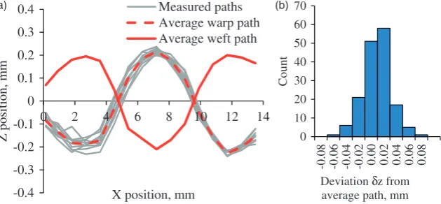
The average yarn path in the z direction (out-of-plane) with strong systematic variation due to weaving, as shown in Figure 2(a), was observed in every warp and weft yarn. The standard deviation ofz from the average path was 22mm, and its measured distribution is shown in Figure 2(b). The deviation of average in-plane (xfor warp and or yfor weft) yarn path from a straight line was within 40mm, while the standard devi-ation from average path was 25mm. The in-plane paths and distribution of deviationyfrom the average path are shown in Figure 3(a) and (b), respectively. A sum-mary of the measurements is given in Table 1.

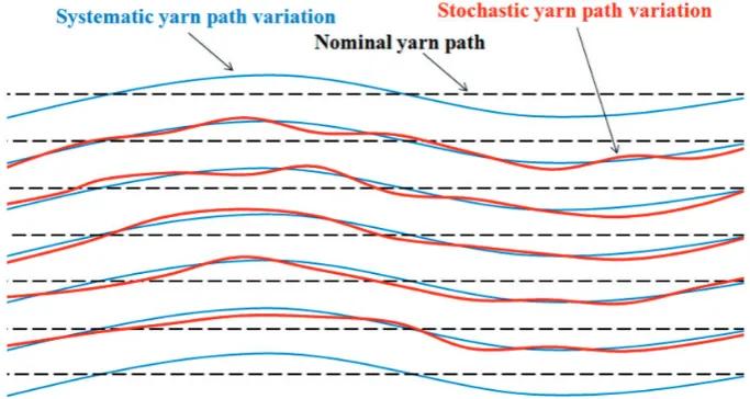
At the same time, the absence of significant variabil-ity at the scale of a single unit cell does not mean absence of variability at the macro-scale. In-plane

variability of the yarns path at the macro-scale can be represented by equation (1) as well. Schematic repre-sentation of the woven reinforcement with systematic and stochastic variabilities of yarn path is shown in Figure 4. Images of the textile surface consisting of vis-ible segments of yarns as shown in Figure 5(a) were processed with an in-house image processing software developed within the MATLAB framework. The warp and weft yarns were separated using a simple thresh-olding technique and then analysed. The watershed algorithm19 was used to find the centres of the yarn segments as a first approximation. The information about the centres was then transferred to a subprogram which operated with subimages of the yarn segments cropped from the overall image. A gradient edge detec-tion filter19was applied on each subimage, and edges of the yarn segment were approximated with a rectangle (Figure 5(b)). The parameters of fitted rectangles were stored as local yarn dimensions, positions and orienta-tions and used to reconstruct yarn paths as shown in Figure 5(c).

Figure 1. m-CT images of manufactured composites with highlighted yarns: Panel #3 (top) and Panel #5 (bottom).

-0.4 -0.3 -0.2 -0.1 0 0.1 0.2 0.3 0.4

(a) (b)

0 2 4 6 8 10 12 14

Z position, m

m

X position, mm

Measured paths Average warp path Average weft path

0 10 20 30 40 50 60 70

-0

.08

-0

.06

-0

.04

-0

.02

0.

00

0.

02

0.

04

0.

06

0.

08

Count

Deviation δz from average path, mm

The described algorithm was applied to three sam-ples of dry textiles with size of 270210 mm each, scanned on a flatbed scanner with resolution of 21mm (1200 dpi). The accuracy of the algorithm was estimated by comparing yarn width measured by micro- and macro-techniques. The width measured by m-CT was 2.4950.068 mm, while image analysis of the

reinforcement surface yielded a width of 2.5200.056 mm for the textile. The small difference between these values confirms the accuracy of the approach.

The structure of the analysed reinforcements was reconstructed using information about yarn segment centre points yielding a model of the paths for every -0.3

-0.2 -0.1 0 0.1 0.2 0.3

(a) (b)

0 2 4 6 8 10 12 14

Y

position, m

m

X postion, mm

Measured paths

Average warp path

Average weft path

0 10 20 30 40 50 60 70

-0.0

8

-0.0

6

-0.0

4

-0.0

2 0

0.0

2

0.0

4

0.0

6

0.0

8

Frequency

Deviation δy from

average path, mm

Figure 3. (a) In-plane yarn paths in Panel #5; (b) deviation of yarn from average in-plane yarn path for all the yarns in Panel #5.

Table 1. Summary of measurements fromm-CT scans.

Panel

Deviation from in-plane average path, mm

Deviation from out-of-plane average path, mm

Width, mm

Height, mm

Random layer shift Panel #1 0.034 0.020 2.572 (0.085) 0.342 (0.023) Panel #3 0.027 0.017 2.516 (0.106) 0.364 (0.029) No layer shift Panel #5 0.025 0.022 2.491 (0.068) 0.352 (0.024)

Figure 4. Schematic representation of systematic and stochastic yarn path variations from the nominal yarn path in woven

yarn. It was found that the yarn paths possessed strong systematic variation from a straight line (as shown in Figure 4) with amplitudes of up to 1.0 mm. Distributions of variations from the average yarn path were close to normal distributions with standard devi-ations of 47–97mm for the textiles. A typical distribu-tion is shown in Figure 6(a). A summary of the measurements is given in Table 2. It should be empha-sised that variability at the meso-scale had an ampli-tude three times higher than the variability at the macro-scale. It makes it possible to assume that the

geometry of the unit cell has negligible variability at the meso-scale when compared to the macro-scale.

The analysis of yarn paths showed that adjacent yarns in the studied reinforcements tend to have similar variation and this similarity was described by correl-ation.20 Correlation between yarn j-th and (jþk)-th yarns was defined as Pearson’s correlation20

C kð Þ ¼

Pn

i¼1y

ðjÞ

i y

ðjþkÞ

i

ffiffiffiffiffiffiffiffiffiffiffiffiffiffiffiffiffiffiffiffiffiffiffiffiffi Pn

i¼1 y

ðjÞ

i

2

r ffiffiffiffiffiffiffiffiffiffiffiffiffiffiffiffiffiffiffiffiffiffiffiffiffiffiffiffiffi Pn

i¼1 y

ðjþkÞ

i

2

r ð3Þ

Autocorrelation of a yarn with itself and autocorrel-ation length was defined as Pearson’s correlautocorrel-ation between pairs of points spaced at a distance ofknodes20

Cað Þ ¼k

Pnk

i¼1 y

ðjÞ

i y

ðjÞ

iþk

ffiffiffiffiffiffiffiffiffiffiffiffiffiffiffiffiffiffiffiffiffiffiffiffiffiffi Pnk

i¼1 y

ðjÞ

i

2

r ffiffiffiffiffiffiffiffiffiffiffiffiffiffiffiffiffiffiffiffiffiffiffiffiffiffiffi Pnk

i¼1 y

ðjÞ

iþk

2

r ð4Þ

Figure 5. (a) Textile image, yarn segments; (b) automatic segment detection; (c) yarn path reconstruction.

-0.40 -0.2 0 0.2 0.4 50

100 150

(a) (b)

Deviation δy, mm

Count

-1 -0.5 0 0.5 1

0 100 200 300

Corellation

Distance in yarn direction, mm Warp corellation Warp autocorellation Weft corellation Weft autocorellation

Figure 6. (a) Experimental and fitted distributions of deviationyfrom mean weft yarn path in Textile #1; (b) correlation and

autocorrelation for warp and weft yarns (averaged over three samples).

Table 2. Summary of measurements from macro-scale images.

Weft variation, mm

Warp variation, mm

Sample 1 0.082 0.096

Sample 2 0.097 0.047a

Sample 3 0.083 0.082

a

Cross-correlation between warp and weft yarns was defined as Pearson’s correlation between the j-th warp andj-th weft yarns

Cc¼

Pn

i¼1y

ðj,warpÞ

i y

ðj,weftÞ

i

ffiffiffiffiffiffiffiffiffiffiffiffiffiffiffiffiffiffiffiffiffiffiffiffiffi Pn

i¼1 y

ðjÞ

i

2

r ffiffiffiffiffiffiffiffiffiffiffiffiffiffiffiffiffiffiffiffiffiffiffiffiffi Pn

i¼1 y

ðjÞ

i

2

r ð5Þ

The graphs showing correlation and autocorrelation of yarns depending on spacing between yarn and nodes are shown in Figure 6(b). It can be seen that the correlation coefficient is high (correlation value of 1.0 shows perfect match of yarns and value of 0.0 shows that paths are independent) which means that adjacent yarn paths were very similar to each other. Autocorrelation showed that the yarn path is independent of itself (i.e. it is not influenced by its own history) after three to four unit cells (about 30–40 mm). Values of autocorrelation length between 30 mm and 110 mm were reported by other research-ers.10,21,22 Average cross-correlation between warp and weft yarns (i.e. effect of variation of warp yarn path of weft yarn path and vice versa) was found to be below 0.1.

It should be made clear that detailed analysis of macro-scale variability was performed on dry reinforcement only whereas handling, cutting, lay-up and resin infusion can potentially change parameters measured from the textile. Analysis of the reinforce-ment geometry at the surface of the composite panels showed that systematic variations are lower than in the dry reinforcement, up to 0.7 mm, but no data were obtained on stochastic variation due to the poor quality imaging obtained from the composites. According to Endruweit et al.23 repetitive specimen handling may decrease the geometrical variability. However, such handling is reduced in the RTM process because the

reinforcement mobility is restricted by inter-layer fric-tion. Therefore, it is expected that the presented statis-tical parameters of dry reinforcement are close to those of finished composite.

Mechanical testing

Specimens from each panel were tested in tension in the warp direction according to the EN ISO 527 standard using an Instron 5985 machine with 250 kN load cell and test speed of 2 mm/min at room temperature (20_{C). A} DANTEC Q400 3D digital image correlation (DIC) system was used to monitor displacements (and therefore strains) in the outer layer of the composites. A facet size (size of subregion for image processing) of 17 pixels was used to correlate images. Strain fields were averaged over all the specimen area in order to obtain the applied aver-age strain. The measured Young’s moduli, Poisson’s ratios and strengths are given in Table 3.

Longitudinal strain fields acquired with DIC system are shown in Figure 7. It can be seen that strains exhibit

Table 3. Summary of mechanical testing.

# of tested samples

Young’s modulus, GPa

Poisson’s ratio

Strength, MPa

Ultimate strain, %

Random layer shift Panel #1 6 55.74 (1.38)

0.069 (0.007)

571.0 (20.5)

1.11 (0.10)

Panel #2 6 55.36

(2.13)

0.082 (0.016)

484.6 (31.0)

1.37 (0.26)

Panel #3 12 55.96

(1.65)

0.054 (0.008)

582.2 (17.6)

1.35 (0.24)

No layer shift Panel #4 9 54.89

(1.02)

0.073 (0.012)

595.9 (25.5)

1.38 (0.13)

Panel #5 8 53.26

(1.23)

0.129 (0.007)

644.6 (74.8)

1.46 (0.27)

Figure 7. Field of longitudinal strain as measured with DIC at

a regular pattern that clearly corresponds to the reinforcement structure. Low strains were observed in the region of longitudinal yarns, and high strains were observed for transverse yarns. In contrast to the strain field in the composite with no layer shift, the strain field measured on a panel with random layer shift has a less pronounced difference between zones for longitudinal and transverse yarns due to the effect of layers in the depth of the laminate, which are shifted and hence give a more even overall laminate response.

Experiments showed notable differences between the stress–strain curves of specimens with different type of layer shift. The stress–strain curve of specimens with no layer shift exhibited a distinctive kink and strongly non-linear behaviour at strains higher than 1% (similar behaviour was observed by Ito and Chou16). At the same time, specimens with random shift exhibited nearly linear stress–strain curves. A proposed explan-ation for non-linearity in composites with no layer shift is simultaneous straightening of longitudinal yarns in all the layers, and a ‘‘push-out’’ of transverse yarns which is identical for all layers. Yarn straightening in composites with random shift also takes place, but it is not followed by ‘‘push-out’’ of transverse yarns as they are restricted in movement by other layers. This effect in laminates with regular shift is strengthened by the regularity of cracks appearing in transverse yarns and creating weak planes.

Another difference in the behaviour was in the levels of delamination undergone by specimens during the testing. Most of the specimens with random layer shift had extensive delamination in all the layers prior the final failure, while specimens with no layer shift exhibited delamination occasionally and only at the misaligned top layers. The same behaviour was observed by Kiasat and Sangtabi24 for woven textiles with areal density similar to that in the present study.

Modelling

Idealised and stochastic geometry models

Analysis ofm-CT data in the previous section revealed that the yarn dimensions do not change through a unit cell, and the in-plane deviations of the yarn path from a straight line are negligible at this length scale. This makes it possible to create a single-layer unit cell model of the woven composite in TexGen software25 by using aver-aged results of the studies. This model can also be used to create multi-layer models of laminates with layer shifts corresponding to those measured withm-CT.

In order to create a stochastic model of a textile reinforcement at the macro-scale, the warp and weft yarns were assumed to vary independently from each other. The yarn paths were assumed to be defined by

equally spaced nodes on their centrelines generated with the OU sheet, i.e. a 2D random field where one direction corresponds to position along the yarns and the other is across them. The probability density func-tion of the OU sheet for a vectorZis expressed by20

p Zð Þ ¼ _{ffiffiffiffiffiffiffiffiffiffiffiffiffiffiffiffiffiffi}1

2NN_{j j}

p exp 1

2ðZÞ

T1_ðZÞ

ð6Þ

whereNis the size of the vector Z, is the vector of mean values assumed to be zero, and is the covari-ance matrix given by the equation

¼2expð1jx1x2j 2y1y2Þ ð7Þ

where is the standard deviation of the OU sheet, 1 and2are inverse correlation lengths andx1,x2,y1,y2 are coordinates of two points.

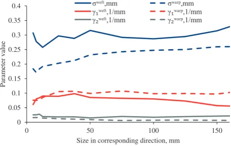
Three parameters introduced in equation (7) are dir-ectly linked to the amplitude of variations (), correl-ation length (2) and autocorrelation length (1). Parameters of the covariance matrix were fitted to experimental data using the maximum log-likelihood estimator.10Estimation was performed using data sub-sets of various sizes starting from just two yarns (1/2 unit cell or 5 mm) up to 150 mm (15 unit cells). Dependency of the OU sheet parameters on textile size is shown in Figure 8. It can be noted that the fitted parameters exhibit some oscillations attributed to the edge effect when minimum and maximum size are used for analysis. Parameters ¼0.2 mm, 1¼ 0.09 mm1, 2¼0.01 mm

1

defined at length 100 mm were chosen as representative for this textile.

The generated realisations of OU sheet characterised system of warp or weft yarns of an arbitrar weft and warp yarns were used to create TexGen models. Each yarn was assumed to have a constant initial width and

0 0.05 0.1 0.15 0.2 0.25 0.3 0.35 0.4

0 50 100 150

Param

eter value

Size in corresponding direction, mm

thickness as determined bym-CT analysis. Small inter-penetrations of yarns which can occur due to the vari-ations of yarn paths were automatically corrected by applying a correction procedure which adjusts yarns dimensions and cross-section orientations as described by Long and Brown.25It should be noted that this pro-cedure does not change the position of the centre of the yarn within TexGen and hence preserves local fibre orientation.

Layer shifts as measured from real samples with m -CT were implemented into the geometrical model by offsetting the layers relative to each other and assuming that there is no additional interpenetration between them, i.e. no nesting was present. Such multi-layered models can be created with both idealised models of textile layers and stochastic models generated as described above. Where stochastic realisations of a layer are used, it was assumed that randomness in each layer is independent from the surrounding layers. However, a stochastic approach was not applied to generation of layer offset itself due to the computa-tional cost arising from the FE analysis of a large number of large models. Though the approach does not create truly random models, the multi-layered models created with this methodology were referred as random layer shift models.

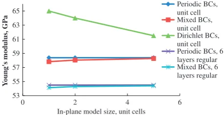
Boundary conditions

An idealised model of a woven composite is an inher-ently periodic structure. Therefore, periodic boundary conditions (BCs)26 can be applied to it in all three dir-ections. In contrast, the geometry of a stochastic model is not periodic and periodic BCs cannot be applied. Other BCs should be used for a proper analysis of a non-idealised woven composite. In this context, three different sets of BCs were applied to single and multi-layer models of an idealised woven composite of vari-ous in-plane sizes: periodic BCs, Dirichlet (prescribed displacement at all edges) and mixed (periodic in

through-thickness direction and Dirichlet in-plane) BCs. The dependency of the Young’s modulus on the model size and BC is shown in Figure 9. Dirichlet BCs increased Young’s modulus by 5% in the case of the largest model size (as explained, e.g. by Hashin and Rosen27) compared with the reference case of periodic BCs. At the same time, mixed BCs gave less than 1% decrease in the Young’s modulus for all considered sizes of model. It can be concluded that, in case when periodic BCs are not applicable due to absence of peri-odicity in the model geometry, it is more appropriate to use mixed BCs rather than Dirichlet BCs due to the lower size dependency of the mixed BCs.

Numerical results

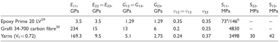
Effect of layer shift on stiffness and strength. The woven composite models were meshed using a voxel meshing technique to avoid possible problems with distorted elements. Validity of the voxel mesh technique was demonstrated earlier for a similar material and loading case.8 Material properties assigned to yarns were obtained using the Chamis micromechanical formulae28 using an intra-yarn fibre volume fraction of 72%. Both matrix and yarn were assumed to be elastic prior to damage initiation which was defined by the maximum stress criterion for yarns and von Mises criterion for matrix. Damage initiation in yarns in longitudinal direction followed by immediate reduction of the lon-gitudinal modulus by factor of 0.001. A simplistic two-parameter damage scheme was chosen for representing gradual degradation of the yarn Young’s modulus in the transverse direction and shear moduli. The matrix Young’s modulus was described by the same scheme. The damage model was coded in UMAT subroutine for Abaqus/StandardTM software. More details on the damage model are given in other papers.6,8 All the material parameters are given in Table 4. Simulations of tensile loading of periodic unit cells were carried out with Abaqus/Standard software using a constant strain increment and mesh of 12012040 voxels for the single layer unit cell and 120120180 voxels for the six-layer unit cell model. Choice of the voxel mesh technique here is dictated by a requirement to generate a large number of FE model in an automatic way which is impossible if a conventional conformal mesh is used as it requires manual check for mesh quality and manual editing to correct for problems. Moreover, it is not always possible to generate a conformal mesh for complex geometries. The voxel mesh technique was validated previously and showed8 that it can be applied for simple loading cases providing the mesh convergence was achieved. Recent studies31 reported strong damage path dependency in voxel models but showed that the voxel approach is suitable for simple 53

55 57 59 61 63 65

0 2 4 6

Y

o

u

n

g's modu

lu

s, GP

a

In-plane model size, unit cells

Periodic BCs, unit cell Mixed BCs, unit cell Dirichlet BCs, unit cell Periodic BCs, 6 layers regular Mixed BCs, 6 layers regular

Figure 9. Effect of BCs on the predicted Young’s modulus

load cases. Mesh convergence was checked over con-vergence of the Young’s modulus and initial damage strain as described in other paper by the present authors.8 Eight-node brick elements (C3D8) were used for the analysis.

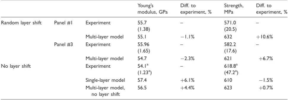
Periodic BCs were applied in the in-plane direction for the multi-layer models and in all three directions for the single layer unit cell model. Resulting stress–strain curves are shown in Figures 10 and 11. Detailed results are presented in Table 5. It can be seen that the single-layer and multi-single-layer unit cell models of a composite with no layer shift yield good predictions resulting in difference of less than 6% for both the Young’s modu-lus and strength. It should be noted that the kink in the stress–strain curve about 1% strain was predicted by both models. However, the multi-layer model yielded closer prediction of the strain when the kink occurs due to more realistic geometry with a finite number of layers and absence of periodic BCs in the through thickness direction. The multi-layer models of the com-posites with random layer shift overpredicted strength by 6–10% of the average experimental value. The Young’s moduli were predicted within 2% of the experimental values.

Effect of yarn path variability. Models of textile with yarn path variability created in TexGen as described in sec-tion Idealised and stochastic geometry models were

meshed using a voxel meshing technique using the same mesh density as in the section on effect of layer shift (12012040 voxels per unit cell). Elastic prop-erties of yarn and matrix materials were assigned according to Table 4. Models of various sizes (11, 22 and 55) were used to study the size effect of a single-layer model. Mixed BCs as described in Boundary conditions section were applied in the in-plane direction. Results of the Monte Carlo simulations with 30 realisations for each size are presented in Figure 12. It can be seen that the Young’s modulus exhibits a size effect, i.e. its value reduces with increase of the model size while its variation decreases. The maximum decrease of the Young’s modulus is only 0.6% and the maximum variation is 0.9%. Predicted variability of the Young’s modulus appears to be several times lower

Table 4. Material properties of constituents and homogenised yarns for the TW model.

E11, GPa

E22¼E33, GPa

G12¼G13, GPa

G23,

GPa 12¼13 23

S11, MPa

S22, MPa

S12, MPa

Epoxy Prime 20 LV29 3.5 3.5 1.29 1.29 0.35 0.35 73a/146b – –

Grafil 34-700 carbon fibre30 234 15 13 6 0.2 0.25 4830 – –

Yarns (Vf¼0.72) 169.3 9.5 5.1 2.75 0.24 0.37 3498 30 42

a

Tension.

b

Compression.

0 100 200 300 400 500 600 700

0 0.5 1 1.5

Stress, MPa

Strain, % Exp

Single-layer model Multi-layer model

Figure 10. Experimental and predicted stress–strain curves for

TW composite with regular layer shift.

0 100 200 300 400 500 600 700

0 0.5 1 1.5

Stress, MPa

Strain, % Experiment

FE prediction

0 100 200 300 400 500 600 700

0 0.5 1 1.5

Stress, MPa

Strain, %

Experiment FE prediction

Figure 11. Stress–strain curves for the models with random

than experimental values which can be up to 3%. It can be noted that there are some realisations exhibiting a Young’s modulus that is higher than the idealised value. This is explained by realisations with almost straight yarns in longitudinal directions and wavy transverse yarns contributing to the increase in Young’s modulus. The other cause of the effect is a slight increase in the fibre volume fraction within an individual model.

The variability of the layer shift was combined with yarn path variability by creating a multi-layer model in the same way as in the section on effect of layer shift and enriching the models by yarn path variation. Monte Carlo simulations were performed on the models of various sizes. The effect of the yarn path variability on the Young’s modulus of multi-layer laminates is pre-sented in Figure 13. This shows the reduction of the average Young’s modulus and its standard deviation in comparison to the Young’s modulus of the idealised composite. As expected, the reduction is greater for the large models as they can include more variations of the yarn paths from the nominal path. At the same time, the standard deviation of the modulus reduction decreases with the size of the model which shows that random models become ‘‘similar’’ to each other. Both graphs seem to plateau at for a model size of 55 unit cells. It also should be noted that the autocorrelation length of the yarn path at the macro-scale was found to be about three to four unit cells, i.e. the in-plane model size of five unit cells covers the autocorrelation length

Table 5. Results of numerical modelling of laminates with various layer shift.

Young’s modulus, GPa

Diff. to experiment, %

Strength, MPa

Diff. to experiment, %

Random layer shift Panel #1 Experiment 55.7 (1.38)

– 571.0

(20.5)

–

Multi-layer model 55.1 1.1% 632 þ10.6%

Panel #3 Experiment 55.96 (1.65)

– 582.2

(17.6)

–

Multi-layer model 54.7 2.3% 621 þ6.7%

No layer shift Experiment 54.1a

(1.23a)

– 618.8a

(47.2a)

Single-layer model 57.4 þ6.1% 610 1.5%

Multi-layer model, no layer shift

56.5 þ4.4% 623 þ0.7%

Note: Standard deviations in parenthesis.

a_{Averaged results for panels #4 and #5.}

56 56.5 57 57.5 58 58.5 59

0 0.2 0.4 0.6 0.8 1

Young's modulus, GPa

P

robabi

li

ty

D

ens

it

y

F

unct

ion

56 56.5 57 57.5 58 58.5 59

0 0.5 1 1.5 2

Young's modulus, GPa

P

robab

ility

D

e

n

sity

F

u

n

c

tio

n

1x1 2x2 5x5

Figure 12. Young’s modulus distribution for 11 RVE (top);

normalised distributions of Young’s moduli for different sized RVEs (bottom).

-0.6 -0.4 -0.2 0 0.2 0.4 0.6 0.8 1 1.2 1.4

0 1 2 3 4 5 6

Reduction of

average

Y

oung's

m

odulus, %

In-plane size of model, unit cells

Modulus reduction (regular) Modulus reduction (Panel #1) Modulus reduction (Panel #3)

Figure 13. Size effect on the Young’s modulus of multi-layer

and the models of this size can be treated as statistically independent. Hence above this size, there should be no further reduction in Young’s modulus and no increase of its standard deviation.

Discussion

This work presents experimental and numerical ana-lyses of two selected geometrical variabilities in a carbon fibre twill weave composite: yarn paths and layer shift variabilities. Experimental analysis is based on multi-scale analysis of the reinforcement’s geometry and mechanical testing of specially prepared samples. Numerical analysis, based on the results of geometric studies, was used to assess the effects of two variabilities in isolation from each other which could be challenging for mechanical testing.

Analysis of geometry variability of a 22 twill weave reinforcement was performed on meso- and macro-scales by means of m-CT and image analysis. The variability at the meso-scale was found to have a magnitude several times smaller than the magnitude of variabilities at the macro-scale. Macro-scale analysis of the textile reinforcement was performed using auto-matic image processing software, making it possible to collect statistics of yarn paths variability from sev-eral samples of the textile. Variation of yarn path from the average path was found to be approximately nor-mally distributed. Correlation characteristics, which describe how fast the yarn path variation decays or changes and hence how fast the mechanical properties change, were calculated as well. It was found that the correlation length in the transverse direction exceeds the size of analysed specimen (200 mm), while the auto-correlation length of yarn paths rapidly decays after three to four unit cells (30–40 mm). A large value of the correlation length in the transverse direction is plausibly explained by tight weaving of the textile where a disturbance in any yarn causes very similar disturbance in adjacent yarns. The autocorrelation length, however, should be related to the elastic proper-ties of the yarns which consist of elastic fibres and hence should behave as elastic beams and have some degree of smoothness and continuity. It is thought that both cor-relation parameters are functions of yarn properties, areal density of textile (spacing between yarns and their width) and weave style. In addition to those vari-ables, handling of textiles can change the geometry of the reinforcement and hence affect variability.23

Mechanical testing showed a significant difference in behaviour of woven laminates with no layer shift and random layer shift. The latter demonstrated almost linear behaviour with a small deviation from this after 0.7% strain while the laminates with no layer shift exhibited significantly non-linear behaviour with a

well defined kink point at about 0.9% strain. This behaviour can be explained by enforced regularity of the structure which magnifies the effect of yarn straightening and regularity of cracks in the transverse yarns which creates weak planes. The observed phe-nomenon highlights the fact that the layer shift has a strong effect on the behaviour of laminates.

Both of the discussed variabilities were also assessed numerically in order to investigate them in isolation. A key aspect of these studies was a unit cell meso-scale model of the composite prepared within TexGen software using averaged meso-scale geometry param-eters collected fromm-CT scans. The model was vali-dated against mechanical experiments of specially manufactured laminates with no layer shift which can be considered as the closest approximation to the idea-lised geometry. The FE analysis on such model showed good qualitative and quantitative agreement with experiments by predicting the kink in the stress–strain curve and yielding the final strength within 2% of the experimental value. Numerical analysis of the non-linear behaviour of the laminates with random layer shift highlighted a qualitative difference in the stress– strain curves caused by the layer shift within a laminate. A possible explanation for the phenomenon of the kink for the case of the no layer shift is proposed: longitu-dinal yarns in the laminate with no layer shift are not restricted from complete straightening and displace the transverse yarns. As for the quantitative difference, the experiments showed that generally the strength of laminates with random layer shift tends to be lower than that of the laminates with no layer shift. However, the standard deviation of the strength of laminates with no layer shift was high and one standard deviation from the mean value included mean values of the strength of the random layer shift laminates. At the same time, numerical analysis showed little difference between strength for laminates with different layer shifts. This means that the quantitative effect of layer shift on the non-linear behaviour of composites is still uncertain.

final failure is dominated by fibre failure mode the model provides good accuracy within 2% of the experi-mental values. The further validation of the model is correct prediction of the kink in the stress–strain curve as discussed earlier. Discrepancy between the numerical predictions and experimental results also can appear due to variability between the samples which is not taken into account for damage modelling.

Yarn path variability was implemented in the idea-lised model of the textile reinforcement by adapting a conventional TexGen model using a random Gaussian field representing deviations from the idealised geom-etry. The Gaussian field was assumed to be represented as OU sheet with properties estimated from reinforce-ment samples. However, only three samples were used to estimate the parameters which can compromise the accuracy of the stochastic model and the results. This technique made it possible to create random realisa-tions of woven composite including multi-layer models. However, a random field of yarn paths gener-ated with the OU sheet lacks the smoothness (in a mathematical sense, i.e. continuity and differentiability) of the realistic yarn paths. This problem was resolved by the automatic refinement procedure within TexGen25 which fits a cubic spline through nodal points of a yarn and then adjusts yarn cross-sections to avoid interpenetrations. Numerical simulations based on the stochastic models showed that the effect of the yarn path variation on the Young’s modulus is not significant. It was found that the variability reduces the Young’s modulus by up to 0.5% and introduces a CoV of up to 0.9%. The results were dependant on the size of the model used for simulations. Larger models yielded a higher reduction of the Young’s modulus and a lower CoV. Larger models (i.e. those containing longer yarns) have higher probability of having more deviations from a straight line and hence a higher prob-ability of larger reduction of modulus. In contrast, the CoV of Young’s modulus reduced with the model size due to higher probability of two large models being similar to each other. The experiments show that the CoV of the Young’s modulus can be up to 3% which is much higher than predicted here. The discrepancy can arise from other sources of variability, e.g. sample orientation during the experiment and accuracy of the experimental procedure.

The combination of the yarn path and layer shift variability showed that the Young’s modulus variabil-ity shows no statistically significant difference between two cases of random layer shift. It should also be noted that no attempt was made to characterise the effect of yarn path variability on the strength of composites. Generally, both of the variabilities combined were found to reduce the Young’s modulus of the composite by as little as 0.5% and introduce a standard deviation

of less than 1% which makes them both insignificant for elastic analysis for this particular reinforcement. However, in the case of a looser reinforcement, yarn path variability may have a more pronounced effect due to larger amplitudes of yarn deviation from nom-inal paths. In contrast, experiments and numerical ana-lyses showed that layer shift variability has a significant effect on the shape of the stress–strain curve.

Conclusions

Performance of a carbon fibre twill weave composite was studied in the light of two structural variabilities: yarn paths and layer shift. Multi-scale analysis of the reinforcement geometry made it possible to establish that meso-scale variabilities are negligible in compari-son to scale variability. It was found that macro-scale variability has a characteristic length of several unit cells (30–40 mm) along the yarns and above 200 mm transverse to the yarns. The latter means that values of stochastic deviations from a straight yarn path of neighbouring yarns are almost identical due to dense weaving of the reinforcement. Mechanical test-ing showed that layer shift is one of the major factors determining the shape of the stress–strain curve, initial elastic modulus and final strength.

Non-linear finite element analysis of the idealised unit cell models under tensile loading yielded a final strength within 11% of the experimental values for all cases. Remarkably good prediction was achieved for the idealised model with no layer shift which was able to capture the kink in the stress–strain curve and pre-dict the final strength within 2% of the experimental value. Numerical analysis of the selected variabilities showed that the quantitative effect of both variabilities is almost negligible (CoV of about 1%) for the elastic analysis of the selected composite. However, the ana-lysis of non-linear behaviour of composites with layer shift variability yielded the same conclusion as experi-ments about its importance for predicting the shape of the stress–strain curve. The question about importance of the yarn path variability for the prediction of the strength of composites remains open.

Declaration of Conflicting Interests

The author(s) declared no potential conflicts of interest with respect to the research, authorship, and/or publication of this article.

Funding

Composites. The authors also wish to express their gratitude for financial support from the University of Nottingham.

References

1. Crookston JJ, Long AC and Jones IA. A summary review of mechanical properties prediction methods for textile reinforced polymer composites. Proc Inst Mech Eng L J Mater2005; 219: 91–109.

2. Daggumati S, Van Paepegem W, Degrieck J, et al. Local damage in a 5-harness satin weave composite under static tension: part II – meso-FE modelling. Compos Sci Technol2010; 70: 1934–1941.

3. Doitrand A, Fagiano C, Chiaruttini V, et al. Experimental characterization and numerical modeling of damage at the mesoscopic scale of woven polymer matrix composites under quasi-static tensile loading.

Compos Sci Technol2015; 119: 1–11.

4. Zhang F, Wu LW, Wan YM, et al. Numerical modeling of the mechanical response of basalt plain woven com-posites under high strain rate compression.J Reinf Plast Comp2014; 33: 1087–1104.

5. Ivanov DS, Baudry F, Van Den Broucke B, et al. Failure analysis of triaxial braided composite. Compos Sci Technol2009; 69: 1372–1380.

6. Green SD, Matveev MY, Long AC, et al. Mechanical modelling of 3D woven composites considering realistic unit cell geometry.Compos Struct2014; 118: 284–293. 7. Phoenix SL and Beyerlein IJ. Statistical strength theory

for fibrous composite materials. In: Kelly A and Zweben C (eds) Comprehensive composite materials. Oxford: Pergamon, 2000, pp.559–639.

8. Matveev MY, Long AC and Jones IA. Modelling of tex-tile composites with fibre strength variability.Compos Sci Technol2014; 105: 44–50.

9. Olave M, Vanaerschot A, Lomov SV, et al. Internal geometry variability of two woven composites and related variability of the stiffness. Polym Compos 2012; 33: 1335–1350.

10. Skordos AA and Sutcliffe MPF. Stochastic simulation of woven composites forming.Compos Sci Technol2008; 68: 283–296.

11. Endruweit A and Long AC. Influence of stochastic var-iations in the fibre spacing on the permeability of bi-directional textile fabrics. Compos Pt A-Appl Sci Manuf2006; 37: 679–694.

12. Mesogitis TS, Skordos AA and Long AC. Stochastic simulation of the influence of cure kinetics uncertainty on composites cure. Compos Sci Technol 2015; 110: 145–151.

13. Vanaerschot A, Cox BN, Lomov SV, et al. Simulation of the cross-correlated positions of in-plane tow centroids in textile composites based on experimental data. Compos Struct2014; 116: 75–83.

14. Vanaerschot A, Cox BN, Lomov SV, et al. Mechanical property evaluation of polymer textile composites by multi-scale modelling based on internal geometry vari-ability. In: 25th international conference on noise and vibration engineering, 4th international conference on

uncertainty in structural dynamics. Leuven, Belgium, 17–19 September 2012.

15. Woo K and Suh YW. Low degree of homogeneity due to phase shifts for woven composites. J Compos Tech Res

2001; 23: 239–246.

16. Ito M and Chou TW. An analytical and experimental study of strength and failure behavior of plain weave composites.J Compos Mater1998; 32: 2–30.

17. Rudd CD. Liquid moulding technologies: resin transfer moulding, structural reaction injection moulding, and related processing techniques. Cambridge: Woodhead Publishing Limited, 1997.

18. Blacklock M, Bale H, Begley M, et al. Generating virtual textile composite specimens using statistical data from micro-computed tomography: 1D tow representations for the binary model. J Mech Phys Solids 2012; 60: 451–470.

19. Wu Q, Merchant FA and Castleman KR. Microscope image processing. Amsterdam: Elsevier/Academic Press, 2008, pp.1–548.

20. Gardiner CW.Handbook of stochastic methods for phys-ics, chemistry, and the natural sciences, 3rd ed. Berlin, New York: Springer-Verlag, 2004, p.415.

21. Vanaerschot A, Cox BN, Lomov SV, et al.

Experimentally validated stochastic geometry description for textile composite reinforcements.Compos Sci Technol

2016; 122: 122129.

22. Gommer F, Brown LP and Brooks R. Quantification of mesoscale variability and geometrical reconstruction of a textile.J Compos Mater2015. DOI: 10.1177/0021998315 617819.

23. Endruweit A, Zeng X and Long AC. Effect of specimen history on structure and in-plane permeability of woven fabrics.J Compos Mater2015; 49: 1563–1578.

24. Kiasat MS and Sangtabi MR. Effects of fiber bundle size and weave density on stiffness degradation and final failure of fabric laminates. Compos Sci Technol

2015; 111: 23–31.

25. Long AC and Brown LP. Modelling the geometry of tex-tile reinforcements for composites: TexGen. In: Boisse P (ed.)Composite reinforcements for optimum performance. Cambridge: Woodhead Publishing Limited, 2011, pp.239–264.

26. Li SG and Wongsto A. Unit cells for micromechanical analyses of particle-reinforced composites. Mech Mater

2004; 36: 543–572.

27. Hashin Z and Rosen W. The elastic moduli of fiber-rein-forced materials.J Appl Mech1964; 31: 223.

28. Chamis CC. Simplified composite micromechanics equa-tions for strength, fracture-toughness and environmental-effects.Sampe Quart1984; 15: 41–55.

29. Prime 20LV Data sheet. 30. Grafil 34-700 Data sheet.