COLD DUST IN HOT REGIONS
Gopika Sreenilayam1, Michel Fich1, Peter Ade2, Dan Bintley3, Ed Chapin3,4,5, Antonio Chrysostomou3, James S. Dunlop6, Andy Gibb5, Jane S. Greaves7, Mark Halpern5, Wayne S. Holland6,8, Rob Ivison6,8,
Tim Jenness3,9, Ian Robson8, and Douglas Scott5
1Department of Physics and Astronomy, University of Waterloo, Waterloo, Ontario, N2L 3G1, Canada 2Cardiff School of Physics and Astronomy, Cardiff University, Queen’s Building, The Parade, Cardiff CF24 3AA, UK
3Joint Astronomy Centre, 660 N. A’ohoku Place, University Park, Hilo, HI 96720, USA 4XMM SOC, ESAC, Apartado 78, E-28691 Villanueva de la Canada, Madrid, Spain
5Department of Physics and Astronomy, University of British Columbia, 6224 Agricultural Road, Vancouver BC V6T 1Z1, Canada 6Institute for Astronomy, University of Edinburgh, Royal Observatory, Blackford Hill, Edinburgh EH9 3HJ, UK
7School of Physics and Astronomy, University of St Andrews, North Haugh, St Andrews, Fife KY16 9SS, UK 8UK Astronomy Technology Centre, Royal Observatory, Blackford Hill, Edinburgh EH9 3HJ, UK
9Department of Astronomy, Cornell University, Ithaca, NY 14853, USA Received 2013 July 3; accepted 2013 December 28; published 2014 January 27
ABSTRACT
We mapped five massive star-forming regions with the SCUBA-2 camera on the James Clerk Maxwell Telescope. Temperature and column density maps are obtained from the SCUBA-2 450 and 850μm images. Most of the dense clumps we find have central temperatures below 20 K, with some as cold as 8 K, suggesting that they have no internal heating due to the presence of embedded protostars. This is surprising, because at the high densities inferred from these images and at these low temperatures such clumps should be unstable, collapsing to form stars and generating internal heating. The column densities at the clump centers exceed 1023cm−2, and the derived peak visual extinction values are from 25 to 500 mag forβ =1.5–2.5, indicating highly opaque centers. The observed cloud gas masses range from∼10 to 103M
. The outer regions of the clumps follow anr−2.36±0.35density distribution, and this power-law structure is observed outside of typically 104AU. All these findings suggest that these clumps are high-mass starless clumps and most likely contain high-mass starless cores.
Key words: dust, extinction – Hiiregions – ISM: clouds – stars: formation – submillimeter: ISM
1. INTRODUCTION
The dust grains in clouds associated with massive star-forming regions absorb the short-wavelength radiation from these stars, heat up, and then re-radiate at far-infrared (FIR) and sub-millimeter wavelengths. For this reason, clouds near Hii regions are good sources of thermal emission. Since thermal radiation from dust is optically thin at FIR and sub-millimeter wavelengths, it is a good tracer of the temperature, density, and gas mass of the clouds, and these properties are significant in characterizing the early stages of star formation. Gas masses are usually determined from CO or dust continuum observations. However, CO is optically thick, its column density subject to an X-factor (Dickman1978) that is not known (the Milky Way value is usually assumed) and is probably sensitive to the local metallicity or background UV field (van Dishoeck & Black 1988; Leroy et al. 2009; Bolatto et al. 2013). Dust mass is usually derived from (sub)millimeter observations on the Rayleigh–Jeans side of the spectral energy distribution (SED), which are sensitive to dust temperatures down to 5–10 K, and in addition are probably also dependent on the metallicity.
Values of dust temperatures and masses estimated from dust emission are subject to the adopted values of the dust emissivity index, β. Values of β in molecular clouds reflect different physical and chemical properties of the clouds, such as the grain size, structure, composition, and environment. At FIR wavelengths, the preferred value of β in the diffuse interstellar medium is∼2 (Draine & Lee1984), and this is the commonly assumed value ofβat long wavelengths. However, a number of observations of cold cores (Shirley et al.2005,2011; Planck Collaboration et al.2011) detected sub-millimeter dust emissivity indices greater than two. In cold, dense regions of
molecular clouds,β can be as steep as∼3.7 (Kuan et al.1996) due to the accretion of ice mantles and grain growth. Toward circumstellar disks, the value ofβcan be as flat as∼1 (Beckwith & Sargent1991). Values of dust emissivity indices as low as∼1 are also observed toward Galactic cores with internal heating sources, perhaps caused by sightline variations in temperature (Juvela et al.2011). Observations of some Class 0 young stellar objects (Kwon et al. 2009) and studies of circumstellar disks around Class II protostars, T Tauri stars (Ricci et al. 2010a, 2010b; Ubach et al. 2012), and young brown dwarfs (Ricci et al.2012) in low-mass star-forming regions suggest even lower values ofβ, less than unity.
Although an accurate measurement ofβ is critical in deter-mining the physical properties of the clouds, the relationship betweenβand dust temperature (Td) is still under debate. Sev-eral studies suggest that β andTd are anti-correlated (Dupac et al.2003; D´esert & et al.2008; Paradis et al.2010). However, such an inverse relation betweenβandTdresulting from least-squares fits to flux densities is sensitive to noise and/or tem-perature variations along the line of sight (Shetty et al.2009a, 2009b). A novel hierarchical Bayesian technique developed by Kelly et al. (2012) finds a weak positive correlation between
β and Td, but they use an unphysical assumption of isother-mal graybody SED parameters. In their comprehensive study to examine the validity of five different potential methods on the shape of theβ–Tdrelation, Juvela et al. (2013) found an inverse
Td–βcorrelation with all the methods, and they noticed a lower bias especially when using the Bayesian method.
One of the best-studied giant molecular cloud (GMC) Hii re-gions is the Orion molecular cloud (OMC)—a moderately lu-minous region (∼5×10⁵Lin the FIR), which is located at a distance of 420 pc. Using the Submillimeter High Angular Res-olution Camera (SHARC), Lis et al. (1998) observed the Orion A molecular cloud, and their studies revealed an average dust temperature of 17±4 K. Dust at temperatures down to 15 K is identified in a clump associated with Orion A (Mookerjea et al.2000) from FIR observations at 138 and 205μm wave-lengths. Mookerjea et al. also found signatures of emission at temperatures between 15 and 20 K, corresponding to cold dust, in a number of Orion clumps, and virtually all of the dust mass is in this cold component. Orion is extensively analyzed using SCUBA by Johnstone et al. in a series of papers: the internal dust temperature of the clumps in the Orion B molecular cloud is in the range 20–40 K (Johnstone et al.2001), whereas the best-fit temperature in the Orion B south molecular cloud is 18±4 K (Johnstone et al.2006), and in Orion A clumps, this is
∼22±5 (Johnstone & Bally2006). However, there is no overall census of the relative amounts of cold dust and warmer dust in clouds such as the OMC. One of the reasons for this is that it has been difficult to observe the extended emission, which is very extended in the case of the OMC.
Cold dust is observed in both low- and high-mass star-forming regions, and the lowest temperatures found toward these regions differ only by a couple of kelvins. The dust temperatures measured toward low-mass star-forming regions are found to be as low as∼7 K in a number of clouds (Evans et al.2001), below∼10–11 K in the pre-stellar cores of the
Oph main cloud (Stamatellos et al.2007), and∼7 K in TMC-1C (Schnee et al.2010). Over the past couple of years, a number of papers have focused on the physical properties of dust near low- and high-mass star-forming regions in the 250–500μm wavelength regime and have found dust temperatures as low as 10 K in molecular clouds. FromHerschel Space Observatory (Pilbratt et al. 2010) data of a collection of low-mass cold, dense globules, Launhardt et al. (2013) obtained temperatures in the range 8–12 K at the interiors. The Balloon-borne Large Aperture Submillimeter Telescope (BLAST; Pascale et al. 2008) observations of an OB-forming complex, Cygnus-X, show some sources with temperatures as cold as∼10 K (Roy et al. 2011). The “Herschel imaging survey of OB Young Stellar objects (HOBYS)” program (Motte et al. 2010) has provided unprecedented details of cold dust associated with Hii regions. Using data from Herschel and other short- and long-wavelength data, the dust temperature map of the Galactic bubble Hiiregion RCW 120, derived by Anderson et al. (2010), shows temperatures down to∼10 K toward local infrared dark clouds (IRDCs). Vela-C, which is a site for both low- and high-mass star formation, shows warmer protostellar sources, with mean dust temperatures of 12.8 K, compared to starless sources with mean dust temperatures of 10.3 K (Giannini et al. 2012). However, not all of these estimates of temperatures can be directly compared because of differences in wavelength coverage, modeling assumptions, and statistical treatments. In particular, the detection of very cold dust requires observations at longer wavelengths. Dust at temperatures below 10 K will have a peak in emission at wavelengths longer than 300μm.
Observations of star formation in other galaxies are dom-inated by regions where clusters of massive stars heat their surrounding region. The properties measured for these regions, such as temperature, luminosity, mass, and star formation effi-ciency, are determined by the interactions of the massive stars
and the molecular clouds near them. Understanding how to turn the observations into measured properties is highly dependent on what we have learned about star formation in similar mas-sive star-forming regions in the Milky Way. However, only a handful of such regions have been well studied, and all of these studies suffer from a number of difficulties. To probe such re-gions, what we really require is higher spatial resolution and longer wavelength observations. In this paper, we use the new SCUBA-2 camera (Holland et al.2013), at 450μm and 850μm wavelengths, to observe a carefully selected sample of massive star-forming regions in the outer Galaxy in order to overcome these problems.
In this paper, we calculate physical properties such as the temperature, density, and mass of the clouds associated with five massive star-forming regions in the outer Galaxy. The clouds are found within 15 of Hii regions, generally with no other significant concentration of interstellar material within many tens of arcminutes. We show the existence of very cold dust, with grain temperatures as low as 7.7 K near very hot massive star-forming regions.
2. OBSERVATIONS AND DATA REDUCTION
We used the SCUBA-2 instrument to observe five regions of massive star formation, centered on the Hiiregions: (1) S148, (2) S156, (3) S159, (4) S305, and (5) S254. Some of these regions only contain one Hii region; some contain as many as five Hiiregions. These Hiiregions are located in the outer Galaxy, and there is very little confusion and contamination with foreground or background cold cores along the line of sight. The distances to our target objects are all well measured, and they are a few kiloparsecs (2.5–5.6) away from the Sun. The target objects are all very bright and could be easily mapped using SCUBA-2, since their angular sizes and separations between their component clumps are small. All of these objects have many observations at other wavelengths from optical to centimeter. The physical properties of all the Hiiregions are summarized in Table 1. Uncertainties on the linear diameter range from∼5% to 27% with a mean uncertainty of∼13% and are primarily due to the uncertainty in the distance to the Hii region.
2.1. SCUBA-2 Data
Name R.A. Decl. d Diameter Diameter Exciting Star
(J2000) (J2000) (kpc) () (pc)
S148 complex
S147 22h55m40s.6 58◦2802.0 5.50±0.89 90 2.44 A4 Va
S148 22h56m05s.7 58◦3055.4 5.60±0.3 90 2.44 O8 Va
S149 22h56m22s.3 58◦3157.1 5.60±0.3 120 3.30 BO Va
S156 complex
BFS15 23h04m42s.6 60◦0456.1 3.0±0.7 61 0.88 . . .
S156 23h05m10s.6 60◦1457.6 2.87±0.75 40 0.56 O8 Vb
BFS18 23h05m47s.3 60◦2406.8 3.0±0.7 59 0.86 . . .
S159 23h15m31s.2 61◦0655.5 2.97±0.31 15 0.22 O9 Vb
S254 complex
S254 06h12m20s.3 18◦0232.5 2.46±0.16 540 6.44 O9.6 Vc
S255 06h13m09s.5 17◦5840.6 2.46±0.16 300 3.58 B0.0 Vc
S256 06h12m39s.3 17◦5648.1 2.46±0.16 120 1.43 B0.9 Vc
S257 06h12m49s.1 17◦5846.1 2.46±0.16 240 2.86 B0 Vd,e
S258 06h13m33s.6 17◦5539.7 2.46±0.16 59 0.7 B1.5 Vc
S305 07h30m07s.0 −18◦3133.5 5.20±1.40 420 10.6 O8.5 V, O9.5 Vf
Notes.The exciting star of S147 is an A4 V star; however, this exciting star cannot produce a Hiiregion and therefore S147 is most likely ionized by a star of a different spectral type.
aCrampton et al. (1978). bRusseil et al. (2007). cChavarr´ıa et al. (2008). dPismis & Hasse (1976). eMoffat et al. (1979). fRusseil et al. (1995).
The SCUBA-2 data were reduced using theStarlinkSMURF (version 1.3.8 for the first three observations and version 1.3.10 for the last two observations) and the iterative map maker (Chapin et al.2013), which is part of the sub-millimeter user reduction facility SMURF (Jenness et al.2011) software pack-age. We followed the recommended “best practice” (Thomas 2013) and used an externally generated zero mask to constrain the map maker and prevent negative bowling.
The final maps were calibrated using flux calibration factors (FCFs) obtained from planet data for the respective observation dates. We derived the FCF using SMURF and the pipeline for combining and analyzing reduced data, PICARD (Jenness et al. 2008),10 which is part of the ORAC-DR (Jenness & Economou1999) pipeline and has the same infrastructure. The FCFs for S156 were derived at both wavelengths using the primary calibrator Mars on the night of the science observation; Uranus was also available as a primary calibrator. Due to bad focusing and atmospheric effects in the Uranus observation (seen primarily at 450μm), which was taken before the period of the science observation in the early evening hours of the observation date, we selected a midnight Mars observation to derive the FCF. In addition, there were standard peak FCF values available from nearly 500 observations at both wavelengths (Dempsey et al.2013). The standard FCFs corresponding to theStarlinkSMURF version at the time of data reduction were (556 ±45) Jy beam −1 pW −1 and (606 ±55) Jy beam −1 pW−1at 850 and 450μm, respectively. The values of the FCFs used for calibrating S156 are 545 Jy beam−1pW−1at 850μm and 563 Jy beam−1pW−1at 450μm, and these are within the uncertainty limits of the standard values. The FCFs for S159 and S148, which were observed on the same day, obtained from both
10 http://www.oracdr.org/oracdr/PICARD
Mars and Uranus, displayed large variations from the standard value, especially at 450μm. We therefore adopted the standard FCFs to calibrate S159 and S148 data.
In finding the FCFs of S305 and S254, we considered two different observations of the planet Mars acquired on the same night. We adopted the FCF derived from the early night Mars observation for calibrating the short-wavelength data. For calibrating the long-wavelength data, we chose a Mars observation near midnight. The values of the FCFs used to calibrate S305 and S254 data at 850 and 450μm wavelengths are, respectively, 566 and 565 Jy beam−1pW−1. The effect of FCF uncertainty on the final fluxes is less than 5% at 850μm and 10% at 450μm (Dempsey et al.2013).
2.2. Role of Background on SCUBA-2 Data
[image:3.612.92.522.76.288.2]field (∼−0.003 Jy beam−1at 850μm and∼−0.009 Jy beam−1 at 450μm) is not significantly different from zero, relative to the noise (∼0.02 Jy beam−1at 850μm and∼0.06 Jy beam−1 at 450μm). Thus, on average, the background emission values are close to zero; therefore, we did not take into account the contribution due to background in the S305 source emission.
In all the target fields of our study, the contribution from the mean value of the background on the source flux is computed to be very low and is neglected in further calculations. Typical on-source signal, especially in the fainter extended regions of S305, is (0.12±0.04) Jy beam −1 at 850μm and (0.36±0.10) Jy beam −1 at 450μm. Note that the absolute value of the mean background emission in S305 is a factor of around 40 (at 850 and 450μm) times smaller than the faint extended on-source emission. For all the target objects, the ratio of the faintest on-source signal to the mean background, on average, is around 41 at 850μm and 17 at 450μm. The total flux due to this offset in the background may be significant for a measure of the integrated flux from these objects, but our main result, the low temperatures of the centers of the clouds, depends on the ratios of surface brightness.
3. PROPERTIES OF THE DUST DERIVED FROM THE IMAGES
Since dust emission at sub-millimeter wavelengths is opti-cally thin, it is a good tracer of the masses of the clouds. In order to estimate temperature, density, and mass, we em-ployed the surface brightness maps of the clouds obtained from SCUBA-2 at 450μm and 850μm wavelengths. In this section we describe the clouds’ physical properties derived using the observed sub-millimeter dust emission maps. The properties are dependent on environmental and instrumental factors, such as calibration, line contamination, knowledge of β, effect of foreground/background, and temperature variations along the line of sight, all of which are examined at the end of Section3.3 and discussed in Section4.
3.1. Dust Emission Morphology
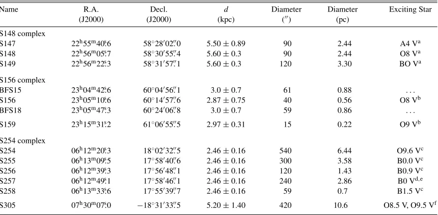
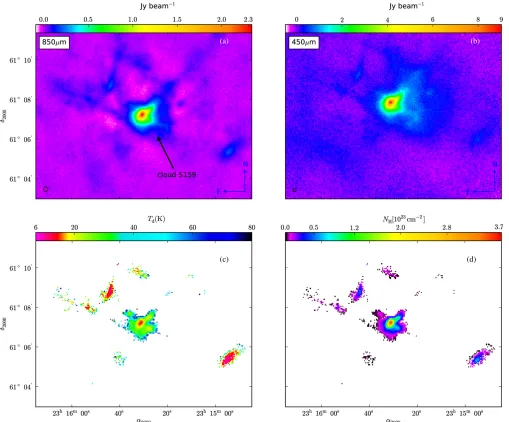
[image:4.612.317.570.72.279.2]The five observed SCUBA-2 maps at 450 and 850μm are displayed in Figures1(a)–5(a) and2(b)–5(b). Hereafter, north is up and east is to the left, with map coordinates in J2000. Due to large-scale sky variations in the 450μm map of S148, we discarded this map from further analysis. A long bar-like cloud whose strongest emission is located at 22h56m45.s8 R.A. and +58◦30 decl., aligned in the north–south direction, is visible in the southeast direction of the cloud associated with the Hii region S148. A third cloud is present in the S148 field at a distance of ∼645 from the map center to the north. Please note that there are no visible optical counterparts for these two unknown clouds in the DSS red image, and therefore these two clouds are most likely some dark clouds along the line of sight or associated with the center cloud. Since the identity and the distances to these clouds are uncertain, we are not taking these two clouds into account in further studies. In the Hii region clouds under discussion, it is apparent that the 450μm maps resemble their 850μm counterparts. The maps presented here are in units of Jy beam−1, and to convert these values to units of MJy sr−1(the other commonly used units), one has to multiply by 185 at 850μm and 426 at 450μm for S159, S148, and S156. For S305 and S254, the Jy beam−1values need to be multiplied by 192 at 850μm and 668 at 450μm to obtain corresponding values in MJy sr−1.
Table 2 Observed Parametersa
Source R.A. Decl. Speak850 Speak450 Tcd
(J2000) (J2000) (Jy beam−1) (Jy beam−1) (K) S148 22h56m17s.2 58◦3101.0 0.50 . . . . . . S156 23h05m08s.9 60◦1448.9 1.09 3.49 11.5 BFS15 23h05m24s.6 60◦0812.8 2.09 5.48 9.5 S156NE 23h06m18s.7 60◦1617.8 0.35 . . . . . . S159 23h15m30s.7 61◦0714.8 2.34 9.03 14.3 S254N 06h12m53s.6 18◦0027.7 4.97 21.7 24.6 S254S1 06h12m53s.8 17◦5924.7 5.33 23.4 23.4 S254S2 06h12m56s.8 17◦5834.0 1.29 4.94 28.6 S305N 07h29m56s.2 −18◦2754.2 0.71 2.22 13.7
S305W1 07h30m00s.3 −18◦3333.5 0.33 0.84 13.8
S305W2 07h30m00s.4 −18◦3109.5 0.26 0.67 14.7
S305W3 07h30m00s.6 −18◦3154.5 0.37 1.01 14.1
S305W4 07h30m00s.9 −18◦3444.5 0.18 0.53 12.9 S305W5 07h30m04s.8 −18◦3103.5 0.29 0.84 13.8 S305E1 07h30m11s.8 −18◦3236.3 0.38 1.04 14.3 S305S 07h30m16s.5 −18◦3551.2 1.10 3.82 16.7 S305E2 07h30m16s.7 −18◦3354.3 0.13 0.37 14.5
Notes.aClouds associated with Hiiregions; peak positions; 850 and 450μm
peak flux densities of the clouds detected in the SCUBA-2 observations of Galactic Hiiregion complexes; and dust temperatures,Tcd(forβ=2), which
come from the peak 450 and 850μm emission. See Figures1–5for maps of these fields.
The observed characteristics of the clouds in the vicinity of the individual Hiiregions are thoroughly discussed in Sreenilayam (2012) and are tabulated in Table2, where the peak positions and flux densities for each object are given. The uncertainties in the peak flux densities are primarily due to uncertainties in the FCF: i.e.,∼5% at 850μm and 10% at 450μm (Dempsey et al.2013). Note that many of these images show more than one area of significant emission. Some of these are more closely associated with other nearby Hiiregions, and we have indicated these with the appropriate names in this table. Some of these emission features are roughly circular and isolated, and later in this paper we identify them as “clumps” and analyze their properties. We presume that these clumps are gravitationally bound collections of cores, and interferometric observations may reveal their fragmentation into individual cores at arcsec resolution. Throughout the paper “cloud” is a general term that, in addition to clumps, refers to less symmetric objects (although some of those might be more correctly described as filaments).
3.1.1. Temperature Distribution
One can derive a pixel-to-pixel dust color temperature map of the clouds by taking the ratio of 450–850μm observed surface brightness maps:
S450(Jy/450 beam)
S850(Jy/850 beam) =
850 450
3+β
exp (17K/Td)−1 exp (32K/Td)−1
(1)
(Kramer et al.2003).
(a) (b)
Figure 1.S148: (a) surface brightness map at 850μm and (b) column density map of S148 at 850μm using temperature derived from assuming aTdof 10 K.
dust grains and is dependent on the dust emissivity index and temperature. In all the temperature maps, the distribution is derived by assuming a constant value for the dust emissivity indexβ. Note that the cloud S148 lacks a good detection at 450μm, and so we were unable to provide a detailed dust temperature map for this cloud. To derive the dust physical properties, we considered a β value of 2, which is often considered to be the standard value at sub-millimeter and millimeter wavelengths (Draine & Lee 1984). The effect of varying emissivity index is discussed in Section3.3in order to investigate the effect of the assumed value ofβon the calculated values of the temperature, density, and mass. The variations in the dust temperature with the flux ratio values are dependent on the adopted values ofβ. If the 450/850 flux ratio is above≈8.3, 11.5, 15.6 forβ =1.5,2,2.5, respectively, then no temperature can be found with the assumptions used here (e.g., uniform dust and dust opacity along the line of sight).
Dust color (450/850) temperature maps of the clouds are calculated using a single dust emissivity index,β = 2.0, and assuming that SCUBA-2 emission at 450 and 850μm are solely originating from dust grains at a single effective temperature. The derived temperatures represent the average of the observed temperatures along the line of sight through the cloud depths (see Figures2(c),3(c),4(c), and5(c)) but with some additional weighting, of an unknown amount, on the hotter outer parts of each cloud.
There are just a few, almost random, points at the outer edges of each structure, where the signal-to-noise ratio (S/N) is low, that are well over 100 K, and they may be just the result of noise. To improve our display of the interior regions, we have set the maximum in the color tables for these figures at 80 K, except for S254, where we have set the maximum to 150 K since the temperatures are much higher in the central regions of this complex. For most of the structures shown, this has resulted in 2 or 3 pixels “disappearing” at the noisy edges, but in the case of S159, approximately 20 “hot” pixels in the outer edge are not shown. In each cloud, a gradient in temperature is observed increasing from the cloud center to the periphery.
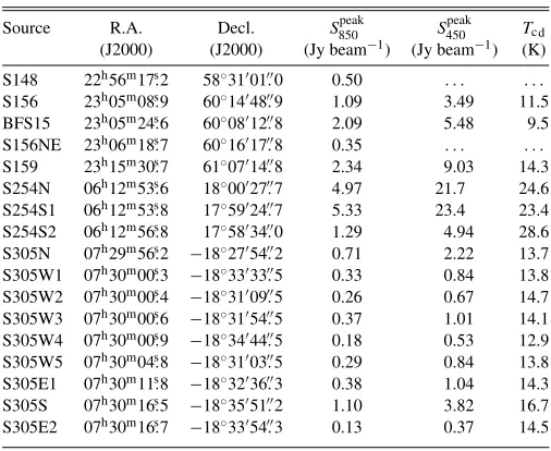
Temperatures are not derived for the cloud associated with S148, due to large-scale sky variations in the 450μm map. We assume a uniform temperature of 10 K throughout S148 to derive the rest of the dust characteristics at sub-millimeter wavelengths. Most of the sources in the S156 field show dust temperature gradients (see Figure 2(c)). The clump near the Hii region S156 is cold, with central temperatures ∼11.5 K, and most of the interior of this clump is below 20 K. The extended region of the clump S156, located in the southeast direction, is relatively warm—reaching on average∼43 K with some pixels at the edge showing temperatures of∼79 K. Note that the clump associated with the Hiiregion BFS15, located in the south, is showing a central temperature of 9.5 K and
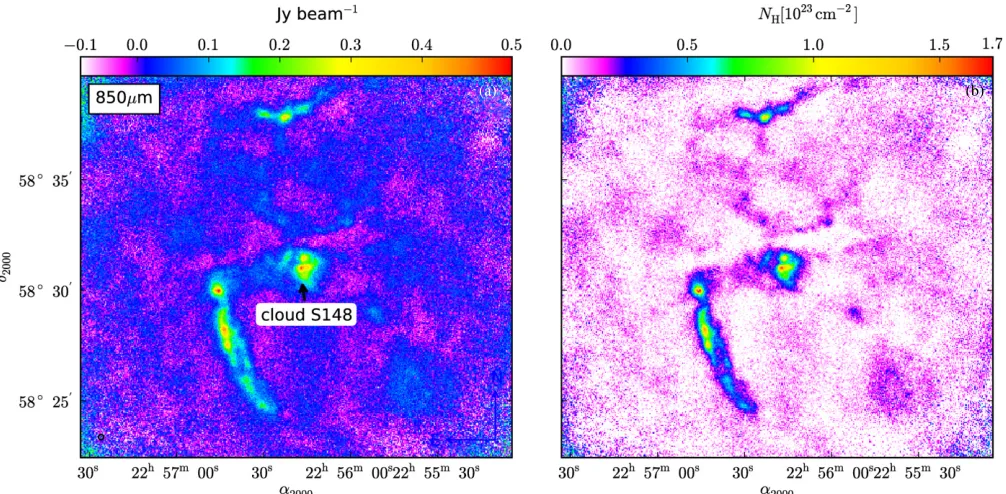
∼28 K, on average, at the outer layers. The 450μm emission of the cloud S156NE is weak (∼1 Jy beam−1) and uniform, while the 850μm emission, although weak, does show a peak in emission. There are a couple of pixels near the center of S156NE showing temperatures below 30 K, possibly due to noise in this generally low S/N region; most of the interior of S156NE shows temperatures of 30–60 K with an increase toward the outer edges. Temperature variations are high in the clump associated with S159, with some of the pixels at the main clump’s outer boundary reaching around 80 K. However, the pixel at the center with the lowest value of Td is at 14.3 K. Outer parts of the clump retain a temperature between 30 and 60 K. All the fragments located in the southwest and northeast directions of the primary cloud show lowest temperatures of around 10 K. The minor fragments visible in the southeast direction are significantly warmer: the temperatures of these regions are found to be above 20 K (see Figure3(c)). S159 is selected for more detailed analysis in Sections3.2and3.3, as this is the largest, and therefore best-resolved, bright, circularly symmetric object.
(a) (b)
[image:6.612.62.559.54.494.2](c) (d)
Figure 2.S156: (a) surface brightness map at 850μm, (b) surface brightness map at 450μm, (c) dust temperature map, and (d) column density map.
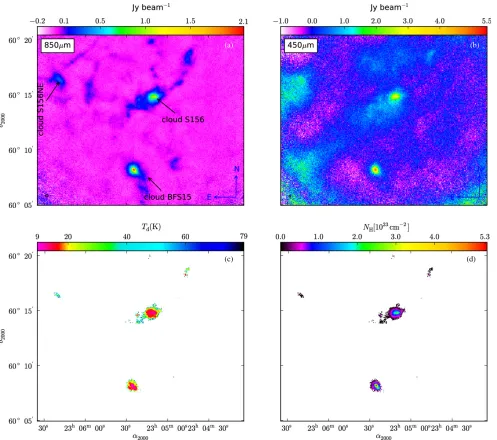
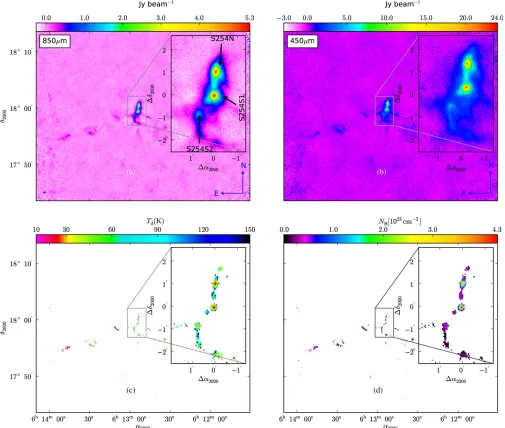
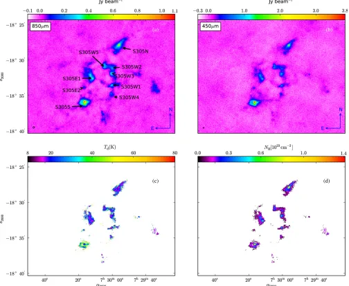
boundary show temperatures beyond 100 K (Figure4(c)). These warmer clumps are most likely associated with the presence of two hot Hii regions on either side of the clouds. This is the hottest environment in our sample, as these clumps are surrounded not only by these two much larger Hii regions, but also by several other large Hii regions in the immediate vicinity. The cloud fragment in the southeast direction, at R.A. 06h13m29s.2 and decl. +17◦5530.8, connected to the Hiiregion S258, shows similar characteristics, with around 23 K dust at its center. However, the cloud located in the southeast direction at R.A. 06h13m47s.0 and decl. +17◦5454.5 shows a relatively colder central temperature of∼11 K. The minimum values of dust temperatures in the clouds of the S305 complex range from∼12 K to 17 K. The clump at the southeast (S305S) is the warmest among all other nebulosities, with central temperatures of∼17 K and grain temperatures reaching∼46 K (on average) at the boundary. All other components of the complex are colder than S305S, with central temperatures ranging from∼12 to 14 K (Figure5(c)).
We identify 15 clouds with good S/N in both 450 and 850μm wavelengths (listed in Table2). We find that 11 of these have
central temperatures,Tcd, below 15 K, and only 3 haveTcdabove 20 K (typical uncertainties inTcdare about 11%). Temperatures below 20 K strongly suggest that there is no central heating source such as an embedded protostar. The average value of the dust temperatures at the centers of all the clouds associated with Hiiregions is∼16 K. The lowest dust temperature is at the center of the clump BFS15 (9.5 K), and the warmest one is in the S254 complex, S254S2 (28.6 K). In all the objects the pixel with the lowest temperature can be driven by noise, and to improve the estimate of the clump, we average over a 14 diameter region; this typically produced a temperature
∼0.7–3.6 K higher. However, in the central clumps of the S254 complex, this produced∼7–25 K higher temperature.
(a) (b)
[image:7.612.55.564.55.477.2](c) (d)
Figure 3.S159: (a) surface brightness map at 850μm, (b) surface brightness map at 450μm, (c) dust temperature map, and (d) column density map.
The majority of the clumps have Td los less than ∼28 K, with temperatures ranging from ∼13–28 K (in the center) to
∼25–50 K (at the edges) except the clumps in the central regions of the S254 complex, where theTd losare higher, with ∼42–54 K at the center and∼90–100 K at the clump boundary. The observedTd losprofile of one of the clumps (near S159) for β = 2 is shown in Figure 7(a) (red curve), where we examine the effect of line contamination andβon our results (as discussed below). The observedTd losdistribution shows a rise in the temperature from the clump’s center to the outer envelope, indicating less input heating in the center, for a constant value of the emissivity index. This feature in our target clumps is most likely attributed to the lack of any central heating source, since cores with increasing temperatures toward smaller radii represent cores that enclose central heating sources (e.g., van der Tak et al.2000). However, in our clumps, there may be external radiation fields, due to the exciting stars of the nearby Hii regions. The only clouds in our sample that would have higher central temperatures due to this are those with lower columns and/or higher external radiation fields, and both of these conditions appear to be true for the sources in the central filament of S254. The range of temperatures found in our study
is slightly higher than that obtained from the low-mass starless core TMC-1C in the Taurus molecular cloud: for aβ of 1.5, they observe dust temperatures ranging from 6 K to 15 K from the center to the outer envelope (Schnee & Goodman 2005), whereas our study on S159 for aβof 2 reveals somewhat higher dust temperatures, ranging from∼14 K to 50 K from the center to the outer envelope.
3.1.2. Column Density Distribution
We calculated the cloud optical depth assuming that the dust emission is optically thin at SCUBA-2 wavelengths. The 850μm map (which is in units of Jy beam−1) is selected to calculate the beam-averaged optical depth. Using the 850μm flux density, the beam area at 850μm, the Planck function at 850μm (B850), and the 450/850 color temperature found above, we can derive the optical depth at 850μm (τ850):
τ850=
F850
ΩbB850(Td)
. (2)
(a) (b)
[image:8.612.55.560.57.485.2](c) (d)
Figure 4.S254: (a) surface brightness map at 850μm, (b) surface brightness map at 450μm, (c) dust temperature map, and (d) column density map. The center for the inset map is at R.A. 06h12m53.s9 and decl. 17◦5924.7.
can follow high column densities, and the column density of hydrogen (H) from 850μm observations can be derived directly from the optical depth using the formula
NH850=
τ850
κ850μmH
, (3)
whereκ850is the mass absorption coefficient, the opacity per unit mass column density, at 850μm. We adoptκ850=0.01 cm2g−1 for a gas-to-dust mass ratio of 100 (opacity per unit dust mass,
κ850,d = 1 cm2 g−1) in the column density calculations of the target objects. The quantityμ(2.33) is the mean molecular weight of the cloud material, andmHis the mass of a hydrogen atom. The measured column density is proportional to the flux at a particular wavelength, as well as the temperature of the dust. We also estimate the extinctionAV at each pixel position
using the widely accepted Milky Way value ofRV = 3.1 in calculations; any change in RV, therefore, changes the value
of visual extinction, AV. For example, if we adopt an RV of
5.5, as found for denser star-forming regions (Mathis 1990;
Draine2003; Whittet2003), in our calculations, then the visual extinction of the clouds will be modified by a factor of∼2.
The maps of the hydrogen column densityNHderived from the 850μm optical depth maps are shown in Figures 1(d), 2(d),3(d),4(d), and5(d). The value ofNH at the outer cloud boundary is very low,≈1021cm−2(S148, S156, S159, S305) and ≈1022cm−2(central regions of the S254 complex). The column densities approach their highest values toward the centers of the clumps. Note that a column density of≈1021cm−2corresponds to an extinction of less than one magnitude, and thus these observed edges of the clouds should match very well with the cloud edges that one would find in an optical image. In fact, in the 450 and especially in the 850μm images we do see slightly farther out than we can accurately compute the temperature and column density, because of low S/N, reinforcing the suggestion that we are seeing the entire cloud.
(a) (b)
[image:9.612.56.560.59.472.2](c) (d)
Figure 5.S305: (a) surface brightness map at 850μm, (b) surface brightness map at 450μm, (c) dust temperature map, and (d) column density map.
S159, S156, and the clump S305S associated with the Hii region S305 also demonstrate peak column densities higher than 1023 cm−2 at the centers. Visual extinction values of the complexes are obtained from their derived column density maps. All the clumps, except those near S148 and S305, show peak visual extinction values above 100. The highest peakAV (283)
is found in the clump near BFS15. In S254N, S254S1, and S254S2, the peak AV values are, respectively, 199, 229, and
41. The other clumps in the sample (near Hii regions S159, S305, and S148) are characterized by peakAV between 63 and
198. The mean central number density,ncof each clump, is the average number density along the line of sight, obtained from the peak column density divided by the size of each clump. The mean central density of the clumps is typically about 8× 104cm−3. However, the central densities of the clumps range over an order of magnitude, from 104 to 105cm−3. The value ofncis lower than the true central density, as it is an average that includes the lower density outer parts of the clump along the line of sight.
The derived clump properties are listed in Table3. The first column gives the source names. The second, third, and fourth columns list the peak values of the optical depth, column density,
Table 3 Properties of the Clumps
Source τ850 NH AV Diameter nc Tcd
(1023cm−2) (mag) (pc) (cm−3) (K)
S148a 6.3×10⁻³ 2.0 86.1 3.56 1.5×10⁴ . . .
S156 9.9×10⁻³ 2.6 136 3.06 6.1×10⁴ 11.5
BFS15 0.02 5.3 283 1.80 1.6×10⁵ 9.5
S159 0.01 3.7 198 1.62 7.4×10⁴ 14.3
S254N 0.01 3.7 199 0.76 1.3×10⁵ 24.6
S254S1 0.02 4.3 229 0.90 1.8×10⁵ 23.4
S254S2 3.0×10⁻³ 0.8 41 0.51 4.9×10⁴ 28.6
S305N 4.6×10⁻³ 1.2 63 1.62 2.3×10⁴ 13.7
S305S 5.4×10⁻³ 1.4 73 2.31 2.0×10⁴ 16.7
Notes.Column 1 lists the clump names associated with the Galactic Hiiregions. Columns 2–4 list the peak values of the optical depth, column density, and visual extinction (using aβof 2) detected toward the centers of the respective clumps. The 850μm size, the central number densities, and the central dust temperatures (forβ= 2) of the clumps are listed in the fifth, sixth, and seventh columns, respectively.
[image:9.612.317.570.516.647.2]Table 4
Properties of the Clumps Usingβ=1.5
Source τ850 NH AV nc Tcd
(1023cm−2) (mag) (cm−3) (K)
S148 . . . . . . . . . . . . . . .
S156 5.1×10⁻³ 1.3 70 3.1×10⁴ 16.9
BFS15 0.01 2.9 154 8.9×10⁴ 12.7
S159 6.2×10⁻³ 1.6 85 3.2×10⁴ 24.9
S254N . . . . . . . . . . . . . . .
S254S1 . . . . . . . . . . . . . . .
S254S2 . . . . . . . . . . . . . . .
S305N 2.0×10⁻³ 0.52 28 1.0×10⁴ 23.1
S305S 1.9×10⁻³ 0.48 26 6.8×10³ 35.1
Notes.Column 1 lists the clump names associated with the Galactic Hiiregions. Columns 2–4 list the peak values of the optical depth, column density, and visual extinction detected toward the centers of the respective clumps, respectively. The central number densities and central dust temperatures of the clumps are listed in the fifth and sixth columns, respectively.
Table 5
Properties of the Clumps Usingβ=2.5
Source τ850 NH AV nc Tcd
(1023cm−2) (mag) (cm−3) (K)
S148 . . . . . . . . . . . . . . .
S156 0.02 4.3 232 1.0×10⁵ 8.9
BFS15 0.03 8.8 469 2.7×10⁵ 7.7
S159 0.03 6.7 360 1.3×10⁵ 10.3
S254N 0.03 8.7 462 3.1×10⁵ 14.2
S254S1 0.04 9.7 518 4.2×10⁵ 13.8
S254S2 7.6×10⁻³ 1.9 104 1.2 ×10⁵ 15.3
S305N 8.2×10⁻³ 2.1 113 4.2×10⁴ 10.1
S305S 0.01 2.7 142 3.7×10⁴ 11.4
Notes.Column 1 lists the clump names associated with the Galactic Hiiregions. Columns 2–4 list the peak values of the optical depth, column density, and visual extinction detected toward the centers of the respective clumps, respectively. The central number densities and central dust temperatures of the clumps are listed in the fifth and sixth columns, respectively.
and visual extinction at the centers of the clumps using the 850μm data, respectively. The size of the clump at 850μm and the average central number density values (nc) are given in the fifth and sixth columns, respectively. The last column provides the values of the central dust temperatures of the clumps. Uncertainties in the diameter and number densities of the clumps are about 18% (due to uncertainties in the cloud distances) and not given in the table. Additional calibration errors of 10% at 450 and 5% at 850μm in the SCUBA-2 flux densities also contribute 11% uncertainties to the values ofτ850,
NH,AV,nc, andTcd(not given in the table). These calculations were repeated forβ =1.5 (see Table4) and forβ =2.5 (see Table5).
3.1.3. Gas Masses from Dust Emission
The gas masses are derived by summing up all the pixel values from the column density maps of the clouds, which are generated from the 850μm dust emission maps, employing a dust temperature distribution assuming a value of β, i.e.,
[image:10.612.43.295.75.198.2]Mgas = μmHNHA, where NH is the total hydrogen column density in cm−2andAis the pixel area in cm2. The gas masses of the clouds are listed in Table6. The first column lists the cloud names. The second, third, and fourth columns list the gas masses corresponding toβ being 2, 1.5, and 2.5, respectively.
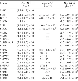
Table 6 Cloud Masses
Source Mgas(M) Mgas(M) Mgas(M)
β=2 β=1.5 β=2.5 S148a (7.3±1.3)×103 . . . . . .
S156 (9.1±1.0)×102 (3.1±0.3×10² (1.7±0.4)×103
BFS15 (9.9±0.6)×102 (4.0±0.2×10² (1.6±0.2)×103
S156NE 11±4 . . . (0.6±0.2)×102
S159 (8.9±0.6)×102 (1.0±0.4)×102 (2.3±0.1)×103
S159C (1.1±0.1)×103 (1.7±0.5)×102 (2.6±0.1)×103
S254N (1.3±0.4)×102 . . . (6.6±1.9)×102
S254S1 (1.1±0.3)×102 . . . (6.0±1.2)×102
S254S2 19±7 . . . (1.3±0.6)×102
S254N and S (2.8±0.5)×102 . . . (1.5±0.2)×103
S254C (4.6±0.7)×102 . . . (1.9±0.3)×103
S305N (8.9±4.0)×102 (2.3±1.0)×102 (1.8±0.9)×103
S305W1 (1.7±0.6)×102 48±7 (3.8±1.5)×102 S305W2 (2.0±0.9)×102 41±9 (4.5±2.4)×102 S305W3 (2.6±1.1)×102 71±17 (5.1±2.7)×102
S305W4 (0.7±0.2)×102 18 (1.5±0.6)×102
S305W5 (2.4±0.6)×102 57±8 (5.4±1.5)×102 S305E1 (7.3±2.3)×102 (1.6±0.4)×102 (1.5±0.6)×103
S305S (5.6±2.1)×102 37 (1.7±0.6)×103
S305E2 15±4 . . . 39±14
S305C (3.1±0.5)×103 6.6×10² (7.1±1.3)×103
Note.aBy assuming a constant temperature of 10 K throughout the cloud.
The uncertainties in the masses are due to the cloud’s shape and they far exceed the flux uncertainties. The mass uncertainties do not include the calibration uncertainties. Flux calibration uncertainties are∼10% at 450 and 5% at 850μm. The letter “C” associated with a cloud in Table6refers to a cloud complex: masses of the S159, S305, and S254 complexes are also included in the table. All the individual clouds in the complexes are massive, with values of gas mass ranging from 11Mto 9.9× 10²M
. The least massive cloud is S156NE, with a gas mass of 11M, while the most massive one is the S305 complex (S305C), with a total mass of 3.1 ×10³M, at least for the
β =2 case. Whenβ =2.5, the least massive cloud is S305E2 (39M) and the most massive one is S305C (3.1×10³M). However, whenβ=1.5, we cannot derive temperature maps of S254C, S156NE, and S305E2, and therefore masses of these clouds are not derived. The difference in mass in all three cases is because of different cloud temperatures corresponding to different values ofβ.
3.2. Analysis of Radial Intensity Profiles
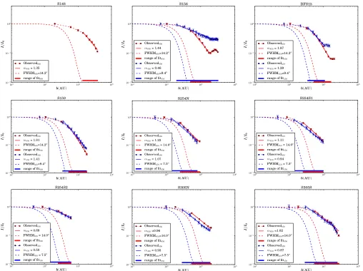
[image:10.612.42.295.281.409.2]Figure 6.Radial profiles of the sources: the 850 (in red) and 450μm (in blue) normalized intensity profiles of the sources plotted as a function of the impact parameter
b(AU) along with the Gaussian main-beam profile at 850 (red dashed curve) and 450μm (blue dashed curve) wavelengths. The thick solid red and blue lines represent the range of the 850 and 450μm fits, respectively.
Normalized, azimuthally averaged radial profiles were con-structed for each intensity map at both SCUBA-2 wavelengths. The images were binned at half the beam width to create equally spaced annuli from the peak intensity of the clumps. Uncertain-ties were estimated from the quadratic sum of the errors due to calibration and the deviation from the azimuthal symmetry at each radial annulus. We calculate the mean value of the intensity
Iν(b) normalized to the peak intensityIν(0) at each radial bin about the impact parameterb(in AU). Following the technique described in Shirley et al. (2000), power-law fits were performed for all clumps using the formIν(b)/Iν(0) =[b/b(0)]−m, with
b(0) corresponding to one-quarter of the beam width. As in Shirley et al. (2000), we only fit each radial profile outside of the FWHM of the beam in each case. The intensity profiles in almost all cases are well fit by a power law (see Figure6). We find a range of values for the power-law indices, with the average value of 1.27±0.37 at 850μm and 0.93±0.31 at 450μm.
The SCUBA-2 beams are much larger than the inner radii of the radial profiles shown in Figure6. Typical physical resolution is greater than∼0.1 pc, or∼2×10⁴AU, which is the 450μm SCUBA-2 beam width of 7.5 at a distance of 2.46 kpc—the distance to the closest object in our sample. The average value of m, obtained by combining the slopes at 850 and 450μm wavelengths, is 1.10±0.34. This value agrees well with the
outer slope of 1 in the intensity distribution of isolated low-mass pre-protostellar cores studied by Ward-Thompson et al. (1994). Our average value ofmis slightly flatter than the mean slope of 1.48±0.35 obtained for low-mass Class 0/I sources by Shirley et al. (2000) and is consistent with the mean inner power-law intensity index of 1.2 found in massive star-forming regions by Beuther et al. (2002).
If we consider an optically thin uniform opacity spherically symmetric clump with Iν(b) ∝ b−m and dust temperature
Td(r) ∝ r−q, then the density profile of the clump ρ(r) will follow r−p, where the power-law indices can be related as
m = p + q − 1 (Adams 1991). The slopes of the radial temperature profiles (corresponding toβ = 2) of our objects, calculated from the dust temperature maps, are used to calculate the density power-law indexp. Since we found an averageqof
−0.26 ±0.10 in five of our clumps, the average value of m therefore translates into an averagep of 2.36±0.35. All the uncertainty values represent uncertainties due to the standard deviation of the sample.
our study have decreasing temperatures toward the centers. Our value of p is steeper than the density power-law index, obtained using one-dimensional (1D) radiative transfer codes, of 1.8±0.4 (Mueller et al.2002—in dense cores associated with massive star-forming regions) and 1.3±0.4 (Williams et al. 2005—in a sample of high-mass protostellar objects). The p values obtained using power-law fits such as 1.6±0.5 (Beuther et al.2002—in a large sample of massive cores in the earliest stages of evolution) and 1.6 ± 0.3 (Pirogov 2009—in high-mass star-forming regions of the southern hemisphere) are also shallower than those from our study. Similarly, 1D radiative transfer studies by Jørgensen et al. (2002) on low-mass Class 0 and Class 1 sources show flatter density power-law indices in the range 1.3–1.9 (±0.2) within∼104AU. However, all these values are dependent on the assumed values of the dust emissivity index,β.
Our power-law indices for densities are steeper than all of these results found by other authors. However, all of these other results are for cores with embedded sources, while our objects do not show any signs of embedded sources. Perhaps this difference in indices is due to this difference in the evolutionary state of the objects. Hydrostatic and hydrodynamic configurations of pressure-bounded cores have density profiles in their outer envelopes that fall off liker−2, similar to what we have found in our studies. The study (Tafalla et al. 2002) of starless cores in low-mass star-forming regions reveals power-law indices ranging from 2 to 4 at large radii, consistent with our mean value ofp. If our objects are truly starless, then we would expect the density structure to flatten in the inner regions. Nevertheless, our resolution (and the source distance) severely limits the ability to see this, and all the power-law structure observed in our study is typically outside of 104AU.
3.3. Caveats
The observed flux densities from sub-millimeter thermal emission are plagued by a number of uncertainties, which can influence the derived dust temperatures and densities. These uncertainties include possible line contamination, variations in the calibration factor, discrepancies in the adopted convolution method, and variations of the value of β. In addition, the assumptions used in the analysis of radial intensity profiles are sensitive to the Rayleigh–Jeans limit.
Spectral line contamination in the SCUBA-2 bolometer bandpasses may be a significant source of uncertainty in the extracted physical properties. Abundant molecules such as CO and its isotopomers embedded in dust clouds are one of the primary sources of dust continuum pollutants at sub-millimeter wavelengths (Gordon1995; Papadopoulos & Allen 2000; Seaquist et al. 2004). The major contributor to line emission in the 850μm band is expected to be the CO(3–2) line at 345 GHz. Methanol and SO2are likely to be significant contributors to the continuum emission—although much weaker than the CO lines, these molecules emit in dozens or even hundreds of separate lines within the bandpass. We can estimate the effect on our results if there is a significant amount of line emission in our 850μm images but none in our 450μm images. This is effectively a “worst” case, because the presence of line emission in the 850μm image would cause us to infer a lower temperature, while such emission in the 450μm image would move our calculated temperatures higher. However, it is possible that in our clouds the line emission is very weak, because the regions are very cold. For example, the CO emission in the 850μm band is theJ = 3 → 2 transition, which is bright in
warm regions. We have CO(3–2) data for some of our objects, and as we discuss below, we find that this is not an important effect in the denser, colder centers of these clouds. The CO has a significant effect on the observed fluxes in the hot outer edges of most of these clouds.
We have obtained CO(3–2) data from the JCMT archives11 for four of our objects: S156, S159, S254, and S305S. The CO(3–2) contribution to the SCUBA-2 850μm dust continuum emission is found to be below∼2%–3% toward the centers of S159, S254N, and S254S, and∼10% at the outermost borders of the clumps. The extended envelopes of the S159 cloud exhibit higher contributions from the CO(3–2) line:∼15%–45% for the northwest and east,∼40%–90% for the northeast envelope. A few pixels at the northwest part of the central S254 cloud show dominant CO(3–2) line contribution,∼30%–60%. Overall, the CO(3–2) line contributes little to the bulk of the S254 cloud. Contamination under ∼15% toward the centers and <40% toward the outer borders of the clumps S156 and S305S is observed. The CO(3–2) line emission contributed∼60%–90% of the SCUBA-2 850μm flux at some parts of the extended envelope of S156. Recent studies on the Perseus B1 clump by Sadavoy et al. (2013) found that CO(3–2) line emission contributed only less than 15% of the 850μm flux on the internally heated regions and less than 1% of the 850μm flux on the colder regions of the B1, with the most significant contribution, ∼90%, at the outflow positions. Studies on a number of nebulae in the Perseus and Orion cloud complexes by Drabek et al. (2012) confirmed less than 20% contribution from the CO(3–2) line emission on the SCUBA-2 850μm flux in regions without outflows and an insignificant contribution from CO(6–5) lines at 450μm dust emission.
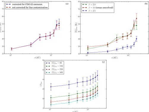
The removal of line-contaminated flux densities from the SCUBA-2 850μm data has only a minor effect on the dust temperatures in the dense clumps (see Figure7(a)): subtraction of the observed S159 CO(3–2) data from the 850μm SCUBA-2 data barely changed the central dust temperatures, although it slightly increased the outer temperatures (Figure 7(a)—blue curve). If there is a higher contribution from CO or from other molecular lines within this band (for example,∼30%), then the clump temperatures alter considerably: removal of an assumed 30% line contamination increased the temperatures by around 93% at the center. However, due to very high 450/850 flux ratio at the edges, the temperatures at the clump edges could not be evaluated. Elimination of the line contribution to the continuum (using the observed CO data) did not change the density power-law index. Although the CO(3–2) emission does not affect the main results of this paper (very cold, dense clumps), it does cause us to slightly underestimate the temperature at the edges of the clouds surrounding the clumps. A more detailed analysis of the CO emission is underway and will appear in a future paper.
Small variations in the adopted value of the FCF have a negligible effect on the results. For example, employing the standard value of FCF to calibrate the S156 map field, by raising the value of FCF by∼2% at 850 and∼7% at 450, caused only
∼4%–5% variations in the central dust temperatures and∼7% variations in the peak dust column densities of the clouds.
Since the 850μm beam solid angle is larger due to the error beam pattern than just the main-beam solid angle and there is large difference in the side-lobe patterns between 450 and 850μm, convolving the 450μm SCUBA-2 map to the 850μm
(c)
Figure 7.(a) Line-of-sight averaged dust temperature (Td los) profiles of the cloud associated with S159, with (red curve) and without (blue curve) line contamination
at 850μm. The blue curve represents temperature obtained from the data corrected for CO(3–2) emission at 850μm, using aβof 2. (b) Variations in theTd losprofile
with different assumed values ofβ. The red curve represents the temperature obtained from the 450/850 ratio map, using aβof 2, after doing cross-convolution (convolving 450μm data to the resolution of 850μm 14.2 primary beam and 850μm data to the resolution of 450μm 9.4 primary beam). Error bars indicate the uncertainty in the temperature due to a combination of calibration and the error in the mean of the temperature distribution in each radial annulus. (c) Variations inβ
corresponding to different possible values ofTdlosfrom 8 K to 50 K. Error bars indicate the uncertainty inβdue to a combination of calibration and the error in
mean of theβdistribution in each radial annulus.
resolution of the JCMT beam, to roughly match the Gaussian main beams at both wavelengths, may lead to some uncertainties in the result. We therefore performed a cross-convolution on one of the clouds (S159), by convolving 450μm data to the resolution of 850μm 14.2 primary beam and 850μm data to the resolution of 450μm 9.4 primary beam as described in Hatchell et al. (2013). The cross-convolution method raised the value of the dust temperature at the center of S159 by around 3 K. However, this method did not make a large increase in the temperature, and all the values obtained from this method are within the uncertainty limits of the temperatures obtained by the method used in this paper (see Figure7(b)).
Variations in the Td los profiles of the clump close to S159, corresponding to different values ofβ, are displayed in Figure 7(b). Since there is some evidence of β > 2 toward low-mass star-forming regions (Schnee et al. 2010; Shirley et al. 2011), we also explored the possibility of β = 2.5 in our calculations. As the value of β increases from 2.0 to 2.5, the Td los profile shifts downward, denoting an anti-correlation between temperature and values ofβ, a very well known effect, discussed by many authors. Our determination
of the temperatures depends on what value ofβ we use in the calculations. The central clump temperatures shift from∼10 K to 14 K as we decrease the value ofβfrom 2.5 to 2.0, indicating cold central regions even in the presence of lowerβ. Similarly, betweenβ of 1.5 and 2.5, Sadavoy et al. (2013) found∼4 K variation in the dust temperature toward the B1-a core. However, whenβis 1.5, the central clump temperature of S159 is∼25 K, but we are unable to plot a temperature profile due to high values of the 450/850 ratio toward the outer layers. The change inβ
barely affects the density power-law index; for example, as we increase the value ofβ from 2 to 2.5, the average value ofp increases by merely 1%. The clouds show another conspicuous feature: regions of lower temperatures correspond to higher column densities if β is uniform throughout the cloud. This feature might imply that the dust grains in the densest regions of the clouds are effectively shielded from the stellar radiation field. As a consequence, grains in these regions are more likely to coalesce than shatter due to lower average kinetic energy (Chokshi et al.1993).
by assuming a constant line-of-sight averaged dust temperature of 8 K, 15 K, 25 K, and 50 K throughout the cloud (see Figure7(c)). The assumed temperatures are considered to be typical temperatures that can be found in different radial layers of the cold GMCs. A radial variation ofβ is observed in all the complexes at all selected temperatures, with low values (e.g.,β ∼1.3 atTd los =50 K) and high values (β ≈3.2 at
Td los=8 K) toward the center of S159. Increasing the assumed temperature from 8 K to 50 K produces on average a decrease inβby 59% toward the center of S159. Much lower values ofβ
(∼0.5) are observed toward the center of the southwest fragment cloud in the S159 complex whenTd los=50 K. Note that the lowest value ofβdetected in the direction of the isolated low-mass star-forming core TMC-1C’s center (Schnee & Goodman 2005) is ∼1.7. At each Td los, one can see lower values of β lostoward the centers of the clouds. Calculating variations in
Td losby assumingβ los∼constant is probably much closer to reality than calculating variations inβ losby assuming that
Td losis constant because the range ofβ losin the latter case is far outside anything actually measured at the sub-millimeter regime (e.g., up to 3.2 in the centers).
The assumption thatm = p+q−1, used in the analysis of radial intensity profiles of the clumps, is valid only in the Rayleigh–Jeans limit, where (hν/k) T. At temperatures below 17 K at 850μm, the Rayleigh–Jeans law breaks down and the interiors of our clumps, whereverTd is less than 17 K, will not satisfy power-law equations. To correct for this, one needs to go back to the Adams (1991) analysis and then change it to account for the low temperatures. However, this will not allow us to directly compare the results to Shirley et al. (2000), Beuther et al. (2002), and Pirogov (2009), as we have done in this paper. Furthermore, modifying the expressions of Adams (1991) is mathematically too challenging for the current paper.
4. DISCUSSION
Stars usually form in locations of cold, dense molecular gas at high densities, over 104 cm−3, and GMCs are ideal sites for such dense concentrations of gas. However, the star formation efficiency, defined as the star formation rate per unit mass of gas, in GMCs is found to be very low, less than 3% (Myers et al. 1986; Lada1987), compared to the star formation efficiency in low-mass star-forming regions. The efficiency of isolated star formation is 9%–15% (Swift & Welch2008) and as high as 30%–50% (Matzner & McKee2000) for clustered low-mass star formation. However, in regions of protostellar outflows, the low-mass star formation efficiency can be 25%–70% (Matzner & McKee2000). Analyzing the clumps within GMCs is therefore important to better understand the low efficiency of their star formation.
The temperatures of the clouds determine the initial stages of star formation. To verify the conditions in the clumps, we calculated the Jeans mass of the clumps (for β = 1.5, 2, and 2.5) using central average number densities, assuming that the gas and the dust temperatures are coupled inside the clumps. At regions of high density, higher than ≈104 cm−3, the gas and the dust temperatures share the same value (Galli et al. 2002; Goldsmith 2001). The derived Jeans masses of the clumps are significantly smaller than the mass of the clumps calculated from the dust emission, suggesting that gravitational attraction overwhelms the thermal pressure, and in the absence of other non-thermal support mechanisms, the clumps will undergo a contraction that in turn is responsible for
a probable eventual collapse. Moreover, there could be cores within these clumps that are collapsing (and still starless); their existence is unknown without higher resolution observations. The support mechanisms may include turbulence or magnetic fields. Ammonia-line observations (to test for turbulence) or observations of sub-millimeter polarization (to look for ordered magnetic fields) would aid in our understanding of how these clumps survive without collapse.
We cannot constrain the values ofβ and temperature simul-taneously using just two wavelengths. We therefore assumed a constantβ to calculate the temperature variations in our cloud samples. However,β may not be uniform in real clouds. Data from shorterHerschelwavelengths (PACS 160 and SPIRE data) with SCUBA-2 data may better constrain the values of the dust temperatures because we can simultaneously calculate temper-ature and β. However, we have not observed the clouds in Herschelbands, and therefore we calculated the physical prop-erties of the clouds with a β of 1.5, 2, and 2.5 to get a pos-sible range of physical values. The inclusion of filtered long-wavelength SCUBA-2 data to Herschel data has been found to increase the reliability of the temperature andβ calculation (Sadavoy et al.2013).Herschelobservations are more sensitive to larger scale structures, but since such structures contribute to both 450 and 850μm emission, it is not clear to what extent this affects our results. In any case, our focus is on the smaller scale structures—the dense clumps—and in order to get color tem-peratures for these, it would be necessary to remove the larger scale structure, which SCUBA-2 already does for us.
We have found cold dust, 9.5–28.6 K forβof 2 and 7.7–15.3 K forβof 2.5, near the Hiiregions considered in this study. But even with very shallow values ofβ, e.g.,β =1.5 everywhere, we have found central temperatures ranging from ∼13 K to 35 K in most of the clouds. The clumps are still unstable to gravitational collapse even with such shallow values ofβ. All these analyses imply that our target clumps are indeed cold and that therefore there is not yet any protostar at their centers. Recent studies by Launhardt et al. (2013) have found similar observational evidence of cold dust (8–12 K) at the interiors, with dominant heating (14–20 K) from the interstellar radiation field (ISRF) at the outer rims, on a number of isolated low-mass starless cloud cores.
Our results of very cold dust near high-mass star-forming regions are consistent with the range of theoretical minimum temperatures found in low-mass starless cores (Evans et al. 2001). Besides dust continuum absorption of the ISRF, Evans et al. (2001) considered different heating mechanisms that will elevate the dust temperature at the center of a starless core/
clump such as cosmic rays, the effect of UV photons that are created following cosmic-ray heating, and collision with warm gas. However, note that all our clouds are farther from the Galactic center than the Evans et al. (2001) clouds—in some cases 50% farther, which means that heating by cosmic rays should be significantly less and our clouds are bigger and denser, and thus heating by ISRF and UV is also considerably less, except, most likely, in the case of the central clumps in the S254 complex.
In nearby, low-mass starless cores, the typical outer dust temperature is ∼20 K for ISRF intensity,G0, ∼few. Typical outer dust temperature in our clumps is∼60 K, and since (for