Understanding seed selection in bootstrapping

Understanding seed selection in bootstrapping

Yo Ehara†∗ Issei Sato‡

†Graduate School of Information Science and Technology ‡Information Technology Center The University of Tokyo / 7-3-1 Hongo, Bunkyo-ku, Tokyo, Japan

∗JSPS Research Fellow

Kojimachi Business Center Building, 5-3-1 Kojimachi, Chiyoda-ku, Tokyo, Japan {ehara@r., sato@r., oiwa@r., nakagawa@}dl.itc.u-tokyo.ac.jp

Hidekazu Oiwa†∗ Hiroshi Nakagawa‡

Abstract

Bootstrapping has recently become the focus of much attention in natural language process-ing to reduce labelprocess-ing cost. In bootstrappprocess-ing, unlabeled instances can be harvested from the initial labeled “seed” set. The selected seed set affects accuracy, but how to select a good seed set is not yet clear. Thus, an “iterative seed-ing” framework is proposed for bootstrapping to reduce its labeling cost. Our framework iteratively selects the unlabeled instance that has the best “goodness of seed” and labels the unlabeled instance in the seed set. Our frame-work deepens understanding of this seeding process in bootstrapping by deriving the dual problem. We propose a method called ex-pected model rotation (EMR) that works well on not well-separated data which frequently occur as realistic data. Experimental results show that EMR can select seed sets that pro-vide significantly higher mean reciprocal rank on realistic data than existing naive selection methods or random seed sets.

1 Introduction

Bootstrapping has recently drawn a great deal of attention in natural language processing (NLP) re-search. We define bootstrapping as a method for harvesting “instances” similar to given “seeds” by recursively harvesting “instances” and “patterns” by turns over corpora using the distributional hypothe-sis (Harris, 1954). This definition follows the def-initions of bootstrapping in existing NLP papers (Komachi et al., 2008; Talukdar and Pereira, 2010; Kozareva et al., 2011). Bootstrapping can greatly

reduce the cost of labeling instances, which is espe-cially needed for tasks with high labeling costs.

The performance of bootstrapping algorithms, however, depends on the selection of seeds. Al-though various bootstrapping algorithms have been proposed, randomly chosen seeds are usually used instead. Kozareva and Hovy (2010) recently reports that the performance of bootstrapping algorithms depends on the selection of seeds, which sheds light on the importance of selecting a good seed set. Es-pecially a method to select a seed set considering the characteristics of the dataset remains largely un-addressed. To this end, we propose an “iterative seeding” framework, where the algorithm iteratively ranks the goodness of seeds in response to current human labeling and the characteristics of the dataset. For iterative seeding, we added the following two properties to the bootstrapping;

• criteria that support iterative updates of good-ness of seeds for seed candidate unlabeled in-stances.

• iterative update of similarity “score” to the seeds.

To invent a “criterion” that captures the character-istics of a dataset, we need to measure the influence of the unlabeled instances to the model. This model, however, is not explicit in usual bootstrapping algo-rithms’ notations. Thus, we need to reveal the model parameters of bootstrapping algorithms for explicit model notations.

To this end, we first reduced bootstrapping al-gorithms to label propagation using Komachi et al.

(2008)’s theorization. Komachi et al. (2008) shows that simple bootstrapping algorithms can be inter-preted as label propagation on graphs (Komachi et al., 2008). This accords with the fact that many papers such as (Talukdar and Pereira, 2010; Kozareva et al., 2011) suggest that graph-based semi-supervised learning, or label propagation, is another effective method for this harvesting task. Their theorization starts from a simple bootstrap-ping scheme that can model many bootstrapbootstrap-ping al-gorithms so far proposed, including the “Espresso” algorithm (Pantel and Pennacchiotti, 2006), which was the most cited among the Association for Com-putational Linguistics (ACL) 2006 papers.

After reducing bootstrapping algorithms to label propagation, next, we will reveal the model param-eters of a bootstrapping algorithm by taking the dual problem of bootstrapping formalization of (Ko-machi et al., 2008). By revealing the model param-eters, we can obtain an interpretation of selecting seeds which helps us to create criteria for the iter-ative seeding framework. Namely, we propose ex-pected model rotation (EMR) criterion that works well on realistic, and not well-separated data.

The contributions of this paper are summarized as follows.

• The iterative seeding framework, where seeds are selected by certain criteria and labeled iter-atively.

• To measure the influence of the unlabeled in-stances to the model, we revealed the model parameters through the dual problem of boot-strapping.

• The revealed model parameters provides an in-terpretation of selecting seeds focusing on how well the dataset is separated.

• “EMR” criterion that works well on not well-separated data which frequently occur as real-istic data. .

2 Related Work

Kozareva and Hovy (2010) recently shed light on the problem of improving the seed set for bootstrap-ping. They defined several goodness of seeds and proposed a method to predict these measures using

support vector regression (SVR) for their doubly an-chored pattern (DAP) system. However, Kozareva and Hovy (2010) does not show how effective the seed set selected by the goodness of seeds that they defined was for the bootstrapping process while they show how accurately they could predict the good-ness of seeds.

Early work on bootstrapping includes that of (Hearst, 1992) and that of (Yarowsky, 1995). Abney (2004) extended self-training algorithms including that of (Yarowsky, 1995), forming a theory different from that of (Komachi et al., 2008). We chose to ex-tend the theory of (Komachi et al., 2008) because it can actually explain recent graph-based algorithms including that of (Pantel and Pennacchiotti, 2006). The theory of Komachi et al. (2008) is also newer and simpler than that of (Abney, 2004).

The iterative seeding framework can be regarded as an example of active learning on graph-based semi-supervised learning. Selecting seed sets cor-responds to sampling a data point in active learn-ing. In active learning on supervised learning, the active learning survey (Settles, 2012) includes a method called expected model change, after which this paper’s expected model rotation (EMR) is named. They share a basic concept: the data point that surprises the classifier the most is selected next. Expected model change mentioned by (Settles, 2012), however, is for supervised setting, not semi-supervised setting, with which this paper deals. It also does not aim to provide intuitive understanding of the dataset. Note that our method is for semi-supervised learning and we also made the calcula-tion of EMR practical.

3 Theorization of Bootstrapping

This section introduces a theorization of bootstrap-ping by (Komachi et al., 2008).

3.1 Simple bootstrapping

Let D = {(y1,x1), . . . ,(yl,xl),xl+1, . . . ,xl+u}

be a dataset. The first l data are labeled, and the following udata are unlabeled. We let n = l+u for simplicity. Eachxi ∈ Rmis anm-dimensional

input feature vector, andyi∈Cis its corresponding

label whereCis the set of semantic classes. To han-dle|C|classes, for k ∈ C, we call ann-sized 0-1 vectory_k= (y1k, . . . , ynk)⊤a “seed vector”, where

yik = 1if thei-th instance is labeled and its label is

k, otherwiseyik = 0.

Note that this multi-class formalization includes typical ranking settings for harvesting tasks as its special case. For example, if the task is to har-vest animal names from all given instances, such as “elephant” and “zebra”, C is set to be binary as C ={animal,not animal}. The ranking is obtained by the score vector resulting from the seed vector

y_animal−y_{not animal}due to the linearity.

By stacking row vectors xi, we denote X = (x1, . . . ,xn)⊤. LetX be an instance-pattern

(fea-ture) matrix where (X)ij stores the value of the

jth feature in the ith datum. Note that we can al-most always assume the matrixX to be sparse for bootstrapping purposes due to the language sparsity. This sparsity enables the fast computation.

The simple bootstrapping (Komachi et al., 2008) is a simple model of bootstrapping using matrix rep-resentation. The algorithm starts fromf₀ def= yand repeats the following steps untilf_cconverges.

1. ac+1=X⊤fc. Then, normalizeac+1．

2. f_c+1 =Xac+1. Then, normalizefc+1.

The score vector after c iterations of the simple bootstrapping is obtained by the following equation.

f =

(

1

m

1

nXX

⊤)c_{y (1)}

“Simplified Espresso” is a special version of the simple bootstrapping whereXij = _maxpmi(i,j_pmi) and we

normalize score vectors uniformly: f_c ← f_c/n,

ac←ac/m. Here, pmi(i, j)def= log_pp_(i(₎i,j_p()_j).

Komachi et al. (2008) pointed out that, although the scoresf_care normalized during the iterations in the simple bootstrapping, when c → ∞, f_c con-verges to a score vector that does not depend on the seed vector y as the principal eigenvector of (₁

m

1

nXX⊤

)

becomes dominant. For bootstrapping purposes, however, it is appropriate for the resulting score vectorf_cto depend on the seed vectory.

3.2 Laplacian label propagation

To makef seed dependent, Komachi et al. (2008) noted that we should use a power series of a ma-trix rather than a simple power of a mama-trix. As the following equation incorporates the score vec-tors((−L)cy) with both low and high c values, it provides a seed dependent score vector with taking highercinto account.

∞ ∑

c=0

βc((−L)cy) = (I+βL)−1y (2)

Instead of using (_m1 _n1XX⊤), Komachi et al.

(2008) usedL def= I −D−1/2XX⊤D−1/2, a nor-malized graph Laplacian for graph theoretical rea-sons. D is a diagonal matrix defined as Dii

def

=

∑

j(XX⊤)ij. This infinite summation of the

ma-trix can be expressed by inverting the mama-trix under the condition that0< β < _ρ(1_L), whereρ(L)be the spectral radius ofL.

Komachi et al. (2008)’s Laplacian label propaga-tion is simply expressed as (3). Giveny, it outputs the score vectorf to rank unlabeled instances. They reports that the resulting score vectorf constantly achieves better results than those by Espresso (Pan-tel and Pennacchiotti, 2006).

f = (I+βL)−1y. (3)

4 Proposal: criteria for iterative seeding

This section describes our iterative seeding frame-work. The entire framework is shown in Algo-rithm 1.

Let gi be the goodness of seed for an unlabeled

instancei. We want to select the instance with the highest goodness of seed as the next seed added in the next iteration.

ˆ_{i= arg max} i

Algorithm 1Iterative seeding framework

Require: y, X, the set of unlabeled instances U, the set of classesC.

Initializegk,i′;∀k∈C,∀i′ ∈U

repeat

Select instanceˆiby (4). Labelˆi. Letk′beˆi’s class. U ←U\{ˆi}

for alli′ ∈U do Recalculategk′,i′

end for

untilA sufficient number of seeds are collected.

Each seed selection criterion defines each good-ness of seedgi. To measure the goodness of seeds,

we want to measure how an unlabeled instance will affect the model underlying Eq. (3). That is, we want to choose the unlabeled instance that would most influence the model. However, as the model parameters are not explicitly shown in Eq. (3), we first need to reveal them before measuring the influ-ence of the unlabeled instances.

4.1 Scores as margins

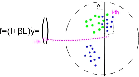
This section reveals the model parameters through the dual problem of bootstrapping. We show that the score obtained by Eq. (3) can be regarded as the “margin” between each unlabeled data point and the hyperplane obtained by ridge regression; specif-ically, we can show that the i-th element of the re-sulting score vector obtained using Eq. (3) can be written as fi = β(yi− ⟨wˆ, ϕ(xi)⟩), where wˆ is

the optimal model parameter that we need to reveal (Figure 1). ϕis a feature function mappingxi to a

feature space and is set to make this relation hold. Note that, for unlabeled instances,yi = 0holds, and

thus fi is simply fi = −β⟨wˆ, ϕ(xi)⟩. Therefore, |fi| ∝ ∥ ⟨wˆ, ϕ(xi)⟩ ∥denotes the “margin” between

each unlabeled data point and the underlying hyper-plane.

LetΦbe defined asΦdef= (ϕ(x1), . . . , ϕ(xn))⊤.

The score vectorf can be written usingΦas in (6). If we setΦas Eq. (6), Eq. (5) is equivalent to Eq. (3).

f =

(

I +βΦΦ⊤

)₋1

y (5)

Figure 1: Scores as margins. The absolute values of the scores of the unlabeled instances are shown as the mar-gin between the unlabeled instances and the underlying hyperplane in the feature space.

ΦΦ⊤=L=I−D−12XXTD− 1

2 (6)

By taking the diagonal of ΦΦ⊤ in Eq. (6), it is easy to see that∥ϕ(xi)∥2 = ⟨ϕ(xi), ϕ(xi)⟩ ≤ 1.

Thus, the data points mapped into the feature space are within a unit circle in the feature space shown as the dashed circles in Figure 1-3. The weight vec-tor is then represented by the classifying hyperplane that goes through the origin in the feature space. The classifying hyperplane views all the points posi-tioned left of this hyperplane as the green class, and all the points positioned right of this hyperplane as the blue gray-stroked class. Note that all the points shown in Figure 1 are unlabeled, and thus the clas-sifying hyperplane does not know the true classes of the data points. Due to the lack of space, the proof is shown in the appendix.

4.2 Margin criterion

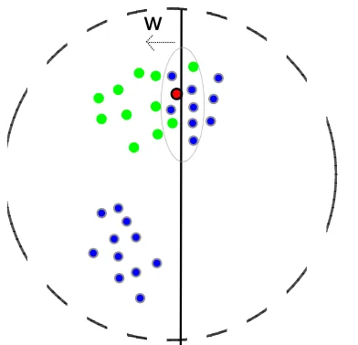
Section 4.1 uncovered the latent weight vector for the bootstrapping model Eq. (3). A weight vector specifies a hyperplane that classifies instances into semantic classes. Thus, weight vector interpretation easily leads to an iterative seeding criterion: an unla-beled instance closer to the classifying hyperplane is more uncertain, and therefore obtains higher good-ness of seed. We call this criterion the “margin cri-terion” (Figure 2).

First, we define gk,i′

def

= |(fk)i′|/sk as the

good-ness of an instancei′ to be labeled as k. sk is the

Figure 2: Margin criterion in binary setting. The instance closest to the underlying hyperplane, the red-and-black-stroked point, is selected. The part within the large gray dotted circle is not well separated. Margin criterion con-tinues to select seeds from this part only in this example, and fails to sample from the left-bottom blue gray-stroked points. Note that all the points are unlabeled and thus the true classes of data points cannot be seen by the underly-ing hyperplane in this figure.

the largest and second largestgk,i′among all classes

as follows:

g_iMargindef= −

(

max k g

Margin k,i′ −2

nd_largest kg

Margin k,i′

) .

(7) The shortcoming of Margin criterion is that it can be “stuck”, or jammed, or trapped, when the data are not well separated and the underlying hyperplanes goes right through the not well-separated part. In Figure 2, the part within the large gray dotted cir-cle is not well separated. Margin criterion continues to select seeds from this part only in this example, and fails to sample from the left-bottom blue gray-stroked points.

4.3 Expected Model Rotation

To avoid Margin criterion from being stuck in the part where the data are not well separated, we pro-pose another more promising criterion: the “Ex-pected Model Rotation (EMR)”. EMR measures the expected rotation of the classifying hyperplane (Fig-ure 3) and selects the data point that rotates the

un-Figure 3: EMR criterion in binary setting. The instance that would rotate the underlying hyperplane the most is selected. The amount denoted by the purple brace “{” is the goodness of seeds in the EMR criterion. This criterion successfully samples from the left bottom blue points.

derlying hyperplane “the most” is selected. This se-lection method prevents EMR from being stuck in the area where the data points are not well sepa-rated. Another way of viewing EMR is that it selects the data point that surprises the current classifier the most. This makes the data points influential to the classification selected in early iteration in the itera-tive seeding framework. A simple rationale of EMR is that important information must be made available earlier.

To obtain the “expected” model rotation, in EMR, we define the goodness of seeds for an instancei′, gi′ as the sum of each per-class goodness of seeds

gk,i′ weighted by the probability that i′ is labeled

ask. Intuitively,gk,i′ measures how the classifying

hyperplane would rotate if the instancei′ were la-beled ask. Then,gk,i′ is weighted by the probability

thati′ is labeled askand summed. The probability for i′ to be labeled as k can be obtained from the i′-th element of the current normalized score vector pi′(k)

def

= |(fk)i′/sk|

∑

k∈C|(fk)i′/sk|

, wheresk is the number

of seeds labeled as classkin the current seed set.

g_iEMR′ def=

∑

k∈C

pi′(k)gk,iEMR′ (8)

The per-class goodness of seedsgk,i′ can be

cal-culated as follows:

gEMR_k,i′ def= 1−

w⊤k

||wk||

wk,+i′ ||wk,+i′||

From Eq. (17) in the proof,w = Φ⊤f. Here,ei′

is a unit vector whosei′-th element is1and all other elements are0.

wk= Φ⊤fk= Φ⊤(I+βL)−1yk(10)

wk,+i′ = Φ⊤fk,+i′ = Φ⊤(I+βL)−1(yk+ei′)(11)

Although Eqs. (10) and (11) use Φ, we do not need to directly calculateΦ. Instead, we can use Eq. (6) to calculate these weight vectors as follows:

w⊤_kwk,+i′ =fk⊤

(

I−D−12XXTD− 1 2

)

fk,+i′ (12)

||w||=

√

f⊤

(

I−D−12XXTD− 1 2

)

f. (13)

For more efficient computation, we cached (I+βL)ei′ to boost the calculation in Eqs. (10)

and (11) by exploiting the fact that yk can be

writ-ten as the sum ofeifor all the instances in classk.

5 Evaluation

We evaluated our method for two bootstrapping tasks with high labeling costs. Due to the nature of bootstrapping, previous papers have commonly evaluated each method by using running search en-gines. While this is useful and practical, it also re-duces the reproducibility of the evaluation. We in-stead used openly available resources for our evalu-ation.

First, we want to focus on the separatedness of the dataset. To this end, we prepared two datasets: one is “Freebase 1”, a not well-separated dataset, and another is “sb-8-1”, a well-separated dataset. We fixed β = 0.01 as Zhou et al. (2011) reports that β = 0.01 generally provides good performance on various datasets and the performance is not keen toβ except extreme settings such as 0 or 1. In all exper-iments, each class initially has1seed and the seeds are selected and increased iteratively according to each criterion. The meaning of each curve is shared by all experiments and is explained in the caption of Figure 4.

“Freebase 1” is an experiment for information ex-traction, a common application target of bootstrap-ping methods. Based on (Talukdar and Pereira, 2010), the experiment setting is basically the same as that of the experiment Section 3.1 in their paper1.

1

Freebase-1 with Pantel Classes, http://www. talukdar.net/datasets/class_inst/

As 39 instances have multiple correct labels, how-ever, we removed these instances from the exper-iment to perform the experexper-iment under multi-class setting. Eventually, we had31,143instances with 1,529features in23classes. The task of “Freebase 1” is bootstrapping instances of a certain semantic class. For example, to harvest the names of stars, given {Vega, Altair} as a seed set, the bootstrap-ping ranks Sirius high among other instances (proper nouns) in the dataset. Following the experiment set-ting of (Talukdar and Pereira, 2010), we used mean reciprocal rank (MRR) throughout our evaluation2. “sb-8-1” is manually designed to be well-separated and taken from 20 Newsgroup subsets3. It has 4,000 instances with 16,282 features in 8 classes.

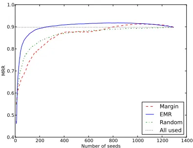
Figure 4 and Figure 5 shows the results. We can easily see that “EMR” wins in “Freebase 1”, a not well-separated dataset, and “Margin” wins in “sb-8-1”, a well-separated dataset. This result can be re-garded as showing that “EMR” successfully avoids being “stuck” in the area where the data are not well separated. In fact, in Figure 4, “Random” wins “Margin”. This implies that the not well-separated part of this dataset causes the classifying hyperplane in “Margin” criterion to be stuck and make it lose against even simple “Random” criterion.

In contrast, in the “sb-8-1”, a well-separated bal-anced dataset, “Margin” beats the other remaining two. This implies the following: When the dataset is well separated, uncertainty of a data point is the next important factor to select a seed set. As “Mar-gin” exactly takes the data point that is the most un-certain to the current hyperplane, “Margin” works quite well in this example.

Note that all figures in all the experiments show the average of 30 random trials and win-and-lose re-lationships mentioned are statistically tested using Mann-Whitney test.

While “sb-8-1” is a balanced dataset, realistic data like “freebase 1” is not only not-well-separated, but also imbalanced . Therefore, we performed ex-periments “sb-8-1”, an imbalanced well-separated dataset, and “ol-8-1”, an imbalanced not-well

sepa-2

MRR is defined asM RR def= _|Q1_|∑_i∈Qr1

i, whereQis

the test set,i∈Qdenotes an instance in the test setQ, andri

is the rank of the correct class among all|C|classes.

3

Figure 4: Freebase 1, a NOT well-separated dataset. Av-erage of 30 random trials. “Random” and “Margin” are baselines. “Random” is the case that the seeds are se-lected randomly. “Margin” is the case that the seeds are selected using the margin criterion described in§4.2. “EMR” is proposed and is the case that the seeds are se-lected using the EMR criterion described in§4.3. At the rightmost point, all the curves meet because all the in-stances in the seed pool were labeled and used as seeds by this point. The MRR achieved by this point is shown as the line “All used”. If a curve of each method crosses “All used”, this can be intepretted as that iterative seeding of the curve’s criterion can reduce the cost of labeling all the instances to the crossing point of the x-axis. “EMR” significantly beats “Random” and “Margin” where x-axis is 46 and 460 with p-value<0.01.

rated dataset under the same experiment setting used for “sb-8-1”. “sl-8-1” have 2,586 instances with 10,764features. “ol-8-1” have2,388instances with 9,971 features. Both “sl-8-1” and “ol-8-1” have8 classes.

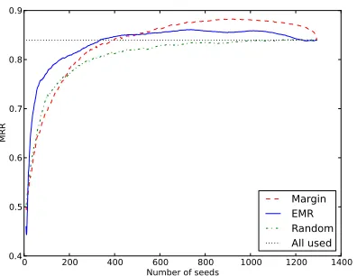
Results are shown in Figure 6 and Figure 7. In Figure 6, “EMR” beats the other remaining two even though this is a well-separated data set. This im-plies that “EMR” can also be robust to the imbal-ancedness as well. In Figure 7, although the MRR of “Margin” eventually is the highest, the MRR of “EMR” rises far earlier than that of “Margin”. This result can be explained as follows: “Margin” gets “stuck” in early iterations as this dataset is not well separated though “Margin” achieves best once it gets out of being stuck. In contrast, as “EMR” can avoid being stuck, it rises early achieving high perfor-mance with small number of seeds, or labeling. This result suggests that “EMR” is pereferable for

reduc-Figure 5: sb-8-1. A dataset manually designed to be well separated. Average of 30 random trials. Legends are the same as those in Figure 4. “Margin” beats “Random” and “EMR” where x-axis is 500 with p-value<0.01.

Figure 6: sl-8-1. An imbalanced well separated dataset. Average of 30 random trials. Legends are the same as those in Figure 4. “EMR” significantly beats “Random” and “Margin” where x-axis is 100 with p-value<0.01.

ing labeling cost while “Margin” can sometimes be preferable for higher performance.

6 Conclusion

Figure 7: ol-8-1. An imbalanced NOT well separated dataset. Average of 30 random trials. Legends are the same as those in Figure 4. “EMR” significantly beats “Random” and “Margin” where x-axis is 100 with p-value<0.01. “Margin” significantly beats “EMR” and “Random” where x-axis is1,000with p-value<0.01.

and improves Espresso-like algorithms.

Our method shows that existing simple “Margin” criterion can be “stuck” at the area when the data points are not well separated. Note that many real-istic data are not well separated. To deal with this problem, we proposed “EMR” criterion that is not stuck in the area where the data points are not well separated.

We also contributed to make the calculation of “EMR” practical. In particular, we reduced the num-ber of matrix inversions for calculating the goodness of seeds for “EMR”. We also showed that the param-eters for bootstrapping also affect the convergence speed of each matrix inversion and that the typical parameters used in other work are fairly efficient and practical.

Through experiments, we showed that the pro-posed “EMR” significantly beats “Margin” and “Random” baselines where the dataset are not well separated. We also showed that the iterative seed-ing framework with the proposed measures for the goodness of seeds can reduce labeling cost.

Appendix: ProofConsider a simple ridge regres-sion of the following form where 0 < β < 1is a positive constant.

minw

β

2 n

∑

i=1

∥yi− ⟨w, ϕ(xi)⟩∥2+∥w∥2. (14)

We defineξi =yi− ⟨w, ϕ(xi)⟩. By usingξi, we

can rewrite Eq. (14) into an optimization problem

with equality constraints as follows:

minw

β

2 n

∑

i=1

ξ_i2+∥w∥2 (15)

s.t.∀i∈ {1, . . . , n};yi =w⊤ϕ(xi) +ξi.(16)

Because of the equality constraints of Eq. (16), we obtain the following Lagrange functionh. Here, each bootstrapping scorefioccurs as Lagrange

mul-tipliers: h(w, ξ,f) def= 1₂∥w∥2 + β₂∑n_i=1ξ2

i −

∑n

i=1(⟨w, ϕ(xi)⟩+ξi−yi)fi.

By taking derivatives of h, we can derive wˆ by expressing it with the sum of eachfiandϕ(xi).

∂h

∂w = 0⇒wˆ =

n

∑

i=1

fiϕ(xi) (17)

∂h ∂ξi

= 0⇒fi =β(ξi=βyi− ⟨wˆ, ϕ(xi)⟩) (18)

Substituting the relations derived in Eqs. (17) and (18) to the equation_∂f∂h

i = 0results in Eq. (19).

∂h ∂fi

= 0⇒ n

∑

j=1

fjϕ(xi)⊤ϕ(xj) + 1

βfi=yi (19)

Equation (19) can be written as a matrix equation using Φ defined as Φ def= (ϕ(x1), . . . , ϕ(xn))⊤.

From Eq. (20), we can easily derive the form of Eq.

(3) as (

ΦΦ⊤+ 1_βI )₋1

y∝(I+βΦΦ⊤)−1y.

(

ΦΦ⊤+ 1

βI )

f =y (20)

2

References

Steven Abney. 2004. Understanding the yarowsky algo-rithm. Computational Linguistics, 30(3):365–395. Klaus Brinker. 2003. Incorporating diversity in active

learning with support vector machines. In Proc. of ICML, pages 59–66, Washington D.C.

Zelling S. Harris. 1954. Distributional structure.Word. Marti A. Hearst. 1992. Automatic acquisition of

hy-ponyms from large text corpora. InProc. of COLING, pages 539–545.

Zornitsa Kozareva and Eduard Hovy. 2010. Not all seeds are equal: Measuring the quality of text mining seeds. InProc. of NAACL-HLT, pages 618–626, Los Angeles, California.

Zornitsa Kozareva, Konstantin Voevodski, and Shanghua Teng. 2011. Class label enhancement via related in-stances. In Proc. of EMNLP, pages 118–128, Edin-burgh, Scotland, UK.

Patrick Pantel and Marco Pennacchiotti. 2006. Espresso: Leveraging generic patterns for automatically harvest-ing semantic relations. In Proc. of ACL-COLING, pages 113–120, Sydney, Australia.

Burr Settles. 2012. Active Learning. Synthesis Lectures on Artificial Intelligence and Machine Learning. Mor-gan & Claypool Publishers.

Partha Pratim Talukdar and Fernando Pereira. 2010. Experiments in graph-based semi-supervised learning methods for class-instance acquisition. In Proc. of ACL, pages 1473–1481, Uppsala, Sweden.

David Yarowsky. 1995. Unsupervised word sense dis-ambiguation rivaling supervised methods. InProc. of ACL, pages 189–196, Cambridge, Massachusetts. Xueyuan Zhou, Mikhail Belkin, and Nathan Srebro.