arXiv:hep-lat/0505023v1 20 May 2005
Practical all-to-all propagators for lattice
QCD
Justin Foley, K. Jimmy Juge, Alan ´
O Cais, Mike Peardon,
Sin´ead M. Ryan, Jon-Ivar Skullerud
∗
(TrinLat Collaboration)
School of Mathematics, Trinity College, Dublin 2, Ireland.
Abstract
A new method for computing all elements of the lattice quark propagator is pro-posed. The method combines the spectral decomposition of the propagator, com-puting the lowest eigenmodes exactly, with noisy estimators which are ‘diluted’, i.e. taken to have support only on a subset of time, space, spin or colour. We find that the errors are dramatically reduced compared to traditional noisy estimator techniques.
Key words: Lattice QCD, Spectral decomposition, Stochastic estimators, Variance reduction
PACS:12.38 Gc
1 Introduction
Hadron spectroscopy has traditionally been performed in lattice QCD by com-puting quark propagators from one or a few points on the lattice (usually the origin) to all other points — so-called point or point-to-all propagators — by inverting the fermion matrix with a point source, and combining the result-ing propagators with appropriate operators to produce the desired hadronic correlators. This method does not require massive computing power, but re-stricts the accessible physics to primarily the flavour non-singlet spectrum.
∗ Corresponding author. Email: jonivar@maths.tcd.ie
Flavour singlet mesons, as well as condensates and other quantities contain-ing quark loops, require propagators with sources everywhere in space, and other methods, notably noisy sources, have been used for this purpose.
Furthermore, point propagators restrict the interpolating operator basis used, for example, to produce early plateaux in effective masses, since a new inver-sion must be performed for every operator that is not restricted to a single lattice point.
Point propagators also throw away a large portion of the information contained in the gauge configurations. It is likely that a limited number of expensive con-figurations with light dynamical fermions will be available in the near future, and it will be highly desirable to extract as much information as possible from these lattices.
All-to-all propagators [1,2,3,4,5,6,7,8,9,10,11,12,13] provide a solution to these problems, but are usually too expensive to compute exactly as this requires an unrealistic number of quark inversions. Stochastic estimates tend to be very noisy and variance reduction techniques are crucial in order to separate the signal from the noise. In this paper we propose an exact algorithm to compute the all-to-all propagator utilising the idea of low-mode dominance corrected by a stochastic estimator which yields the exact all-to-all propagator in a finite number of quark inversions. Some preliminary results were presented in Ref. [14].
The structure of the paper is as follows: In Sec. 2 we describe the principles of the method, and the notation we will use. Sec. 3 describes how QCD cor-relators, and meson two-point functions in particular, are computed in this framework. In Sec. 4 we present results for the meson spectrum, including P-waves and static–light mesons, using this method, and compare these with results using traditional methods. Finally, in Sec. 5 we present our conclusions.
2 Theory and notation
In the following, latin indices i, j, . . . denote colour; greek indices α, β, . . . de-note spin. Indices in brackets dede-note eigenvectors and dilution indices, while indices in square brackets denote independent noise vectors; all of these will be introduced in the following. We useDu, vEto denote the inner product (dot product) of two fermion vectors u and v,
D
u(t), v(t)E≡ X
~ x,α,i
If thet-argument is absent from either of the vectors, the product is taken to be a global dot product, i.e. summed over all t.
2.1 Noisy Estimators and Dilution
The standard method of estimating the all-to-all quark propagator is by sam-pling the vector space stochastically. One generates an ensemble of random, independent noise vectors, {η[1],· · ·, η[Nr]}, with the property
hhη[r](x)⊗η[r](y)†ii=δx,y, (2)
where hh· · ·ii is the expectation value over the distribution of noise vectors. Each component of the noise vectors has modulus 1,
ηiα(x)∗ηiα(x) = 1 (no summation). (3)
The solution vectors ψ[r] are obtained in the usual way,
ψ[r](x) =M−1η[r](y). (4)
The quark propagator from any point x to any other point y is given by
M−1(y, x)ij
αβ =hhψ[r]⊗η[†r]ii ij
αβ = limN
r→∞
1
Nr Nr
X
r
ψiα [r](y)η
jβ [r](x)
†. (5)
This method is noisy because it relies on delicate cancellations in the O(1) noise over many samples to find the signal, which falls off exponentially with the separation. We propose to remove the O(1) random noise by “diluting” the noise vector in some set of variables (j) such that η = P
jη(j), resulting
in an substantial reduction in the variance. A particularly important example of dilution for measuring temporal correlations in hadronic quantities is “time dilution” where the noise vector is broken up into pieces which only have support on a single timeslice each,
η(~x, t) =
N t−1 X
j=0
η(j)(~x, t), (6)
where η(j)(~x, t) = 0 unless t =j.
Each diluted source is inverted, yieldingNdpairs of vectors,{ψ(j), η(j)}, which
then gives an unbiased estimator ofM−1 with asingle noise source,
Nd−1
X
i=0
ψ(i)(~x, t)⊗η(i)(~x
0 5 10 15 20
t/a
0 2 4 6
log C(t)
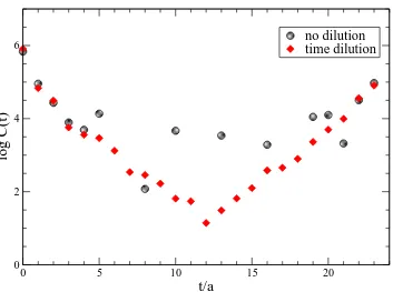
[image:4.612.96.449.65.328.2]no dilution time dilution
Fig. 1. The pseudoscalar propagator computed with and without time dilution.
We show the effect of time dilution on a pseudoscalar propagator on a 123×24 lattice in Fig. 1. The circles are the average of 24 noise sources without any dilution and the diamonds are from a single noise source which has been time-diluted. This particular scenario is analogous to the “wall source on every timeslice” method used by the authors of Ref. [15] to estimate the disconnected diagrams appearing in hadronic scattering length calculations. Our method is, however, more general and can be extended to the spin, colour and space components of the source vector.1 The “homeopathic” limit of the dilution procedure, where we have one noise vector for each time, space, colour and spin component, results in theexactall-to-all propagator in a finite number of steps, because of the property of Eq. (3), see Fig. 2. This limit cannot be reached in practice on realistic lattices, but the path of dilution may be optimised so that the noise from the gauge fields dominate the errors in the hadronic quantities of interest with only a small, manageable number of fermion matrix inversions.
2.2 Spectral Decomposition
In the following we will make use of the hermitian Dirac operator Q≡ γ5M, whereM is the usual Dirac operator. The quark propagator isM−1 =Q−1γ
5,
1 A dilution scheme that includes spin and colour, but not time dilution, was
0 Nmax
N
dilutionerror
[image:5.612.103.448.69.339.2]1/√N
Fig. 2. A cartoon of possible deviations of the stochastic estimates of the exact solution (at Ndil=Nmax) for different dilution paths. Simply adding noise vectors
will give a 1/√N behaviour. We have found that simple dilutions typically follow the behaviour exhibited by the bottom curve.
where Q−1 is given by a sum over all eigenmodes,
Q−1(y, x) =XN i
1
λi
v(i)(y)
⊗v(i)(x)†. (8)
Here, Qv(i) = λ
iv(i) and N is the rank of the matrix. Computing all these
eigenvectors is clearly not feasible; however, theoretical arguments, supported by numerical evidence [16,9,10], suggest that much of the important infrared physics in hadronic interactions is encoded in the low-lying eigenmodes. Trun-cating the sum in Eq. (8) at some finite N → Nev should thus yield a good estimate of the quark propagator for practical purposes. Such a truncation does, however, violate reflection positivity, making it mandatory to correct it.
2.3 Hybrid Method
method with noise dilution is a natural way to accommodate both of those concerns.
First, we note that the exactNevlow eigenmodes obtained separately naturally divide Q into two subspaces, Q=Q0+Q1, defined by
Q0 = Nev
X
i=1
λiv(i)⊗v(i)†, Q1 = N X
j=Nev+1
λjv(j)⊗v(j)†. (9)
Similarly, the quark propagator is broken up into two pieces, Q−1 =Q
0+Q1, where Q0 is the truncated version of Eq. (8) and Q1 = Q−1P
1, where P1 is the projection operator
P1 =1− P0 =1− Nev
X
j=1
v(j)
⊗v(j)†. (10)
We correct the truncation and estimateQ1 using the stochastic method,Q1 = hhψ[r]⊗η[†r]ii withNr noise vectors,{η[1],· · · , η[Nr]}. The solutions are given by
ψ[r]=Q1η[r]=Q−1
P1η[r]
. (11)
We now apply the idea of dilution to the stochastic estimation of Q1. Each random noise vector,η[r], that is generated will be diluted and orthogonalised (with respect to v(i)) so that it can be used to obtainψ
[r]. In other words, we now have the following set of noise vectors:
n
η[1](1),· · ·, η[(1)Nr]
,· · · ,η(Nd)
[1] ,· · · , η (Nd)
[Nr]
o
where the upper indices denote the dilution and the lower indices label the different noise samples. Note that the noise vectors are mutually orthogonal due to the dilution before an average over different random vectors are taken, i.e.,
η[(ri)](~x, t)⊗η[(sj])†(~y, t′) = 0 for alli
6
=j . (12)
This results in smaller variance than the standard method which mixes noise, as Eq. (2) shows.
There is a natural way to combine the two methods to estimate the all-to-all quark propagator. The similarity in the structure of Eq. (8) and Eq. (5) suggests that one construct the following “hybrid list” for the source and solution vectors:
w(i)= (
v(1)
λ1
,· · · ,v
(Nev)
λNev
,P1η(1),· · ·,P1η(Nd) )
(13)
u(i) = (
v(1),· · · , v(Nev)
, ψ(1),· · · , ψ(Nd)
)
0 5 10
t/a
0 0.2 0.4
am
eff
Nev= 50 Nev= 100
Hybrid method N
[image:7.612.96.445.55.313.2]ev= 100
Fig. 3. The pion effective mass from 50, 100 eigenvectors and from the hybrid method with 100 and a time-diluted noise vector.
where the indices run over NHL=Nev+Ndelements. The unbiased, variance
reduced estimate of the all-to-all quark propagator (for a single random noise vector) is then given by
NH L
X
i=1
u(i)(~x, x
4)⊗w(i)(~y, y4)†γ5. (15)
Note that defining w(i) without the projector P
1 on the η-vectors in Eq. (13) also gives an unbiased estimator, which may however have a different variance. Using the pion as an example, we can demonstrate how positivity is recovered from the truncated propagator. In Fig. 3, we show the effective mass from the truncated propagator and from the hybrid method with a time, spin, colour and space (even-odd) diluted noise vector. The truncated propagator, yielding an effective mass that approaches the asymptotic value from below, is corrected by the addition of the diluted noisy propagator.
3 Implementation for QCD correlators
Besides expanding the range of applications accessible in lattice QCD, all-to-all propagators make the construction of hadronic interpolating operators considerably simpler. With the (local) meson creation operator
a meson propagator is constructed using traditional, point-to-all propagators as follows,
CΓ(~x, t;~0,0) = TrM−1(~x, t;~0,0)Γγ5 M−1(~x, t;~0,0)†γ5Γ¯. (17)
This construction, where the local operators are traded for non-local objects constructed from the quark propagators, may work well as long as we restrict ourselves to operators localised at a single lattice site. However, an extended source operator involves connecting quark propagators from sites in the vicin-ity of the source site. This requires at least an additional inversion and entan-gles the matrix inversion and operator construction stages: to a certain extent, the matrix inversion requires knowledge of the operators to be used.
All-to-all propagators eliminate this complication as both source and sink operators are constructed purely from local vectors,
O(Γi,j)(~x, t) =w (i) [1](~x, t)
†γ 5Γu(
j)
[2](~x, t). (18)
The extra factor of γ5 comes from the use of the hermitian Dirac matrix,
γ5M. Two pairs of vectors, (w[1], u[1]) and (w[2], u[2]), are needed for the two independent noisy estimators of the two propagators. Γ can now denote an extended operator acting on the vector u. For complicated operators such as those used to project out hybrid or exotic states, this is a much needed simplification. For example, an interpolating operator for the exotic hybrid 1−+can be constructed from combinations of gluonic paths projecting out the relevant quantum numbers [17]. One term in such a sum may be
w[i](~x)†U
z(~x)Uy(~x+ ˆez)Uz†(~x+ ˆey)u[j](~x+ ˆey), (19)
where the common t-index is suppressed. A standard P-wave state may for example be constructed using
O(i,j)P(~x, t) = w(i)(~x, t)†γ5(Dku(j))(~x, t), (20)
where
Dku(j)(~x, t) =Uk(~x, t)u(j)(~x+ ˆek, t)−u(j)(~x, t). (21)
Using all-to-all propagators, correlation functions are also constructed in an intuitive manner. Hadronic correlation functions are obtained from interpo-lating operators sitting at different time slices, e.g.
CAB(δt) =X t
NH L
X
i,j
O[1(i,j,2])A(t)O (j,i)B
[2,1] (t+δt), (22)
where
O[1(i,j,2])A(t) = X
~x
w[2](i)(~x, t)†γ5ΓAu([1]j)(~x, t)≡ D
w[2](i)(t), γ5ΓAu([1]j)(t) E
and
O([2j,i,1])B(t+δt) = D
w([1]j)(t+δt), γ5ΓBu( i)
[2](t+δt) E
, (24)
for isovector two-point correlators. The correlator is constructed as a product of these meson operators on different time slices. The operators ΓA,B may
now also include phases for momentum projections. As a consequence, once the hybrid list vectors have been constructed, correlation functions for any operator can be computed without any additional inversions.
3.1 Noise recycling
We can take advantage of having saved different random source/solution sam-ples by reusing them in the contraction. In other words, one can generateNR
samples of noise vectors,η[r], save the corresponding solutions,ψ[r]to disk and perform the contraction,
CAB(t, t0) = X
r<s D
w[r](t),ΓAu[s](t) ED
w[s](t0),ΓBu[r](t0) E
, (25)
yielding∼N2
R samples of the correlation function. The errors correspondingly
decrease faster than the naive 1/√NR, although the measurements are
some-what correlated. We have seen in our preliminary tests that the error reduction is comparable to some dilution choices. It is clear that if one can afford to save the noise and solution vectors onto disk, then this is a straightforward method of variance reduction for mass-degenerate mesons.
3.2 Improving Performance
When constructing one of these hadron operators, such as Eq. (23), on a particular time slice t and for a particular operator A, the hybrid technique can be manipulated for computational efficency.
Firstly, compute (and store)
z[1](j)(~x, t) = γ5ΓAu([1]j)(~x, t),∀j. (26)
What now remains for the calculation of the time-slice elements of (Eq. 23) is
NHL×NHL dot-products of spinors on a time slice, since
O[1(i,j,2])A(t) = X
~ x
w[2](i)(~x, t)†z(j)
[1](~x, t)≡ D
We note that time dilution is taken as a minimum requirement in the case of meson two-point functions and that the w(i) hybrid list is naturally divided between our two vector spaces, since
w(i)= (
v(1)
λ1
,· · · ,v
(Nev)
λNev
,P1η(1),· · ·,P1η(Nd) )
. (28)
If we evaluate (and store)
D
w[2](i)(t), z[1](j)(t)E= 1
λi D
v[2](i)(t), z[1](j)(t)E ,∀i≤Nev,∀j , (29)
the elements that remain to be computed are
D
η[2](i)(t),(1− P0)z[1](j)(t) E
=Dη([2]i)(t), z[1](j)(t)E−
Nev
X
k=1
α([22]ik)Dv([2]k), z([1]j)(t)E, (30)
where
α[22](ik) =Dη[2](i)(t), v[2](k)E=Dη[2](i), v([2]k)E. (31)
The first term only needs to be computed ifη[2](i)(t) has support on the relevant time slice. The second term is simply a weighted sum over terms from the eigenvector space of w(i) that have already been calculated. The weights are given by global dot products of quark vectors which can be calculated exter-nally to any particular time slice or operator: Since each η has support on only a single time slice, the global dot product is equal to the dot product of
v with the time-slice restrictedη(t).
This method also reduces the amount of storage required for the noise quark-fields by a factor of Nt since only the supported time slice needs to be stored
on disk, all others being identically zero. This argument is easily extended to include the conjugate operator and all required momenta.
Once the general routine to construct a operator fieldO[(k,li,j])A(t), as in Eq. (23), and the summation over the hybrid list indices required in Eq. (22) are in place, the method becomes a black box to the end user. From Eq. (26), we see that this user need only supply the subroutines to create the required hadron operators from the quark, antiquark and gluon fields on a time slice for each of the required operator fields. These routines would only contain the operations to be performed on the quark field, such asDjψ, and have no reference to the
hybrid lists.
For isoscalar mesons, the disconnected part of the propagator must be in-cluded, yielding the following contraction,
CΓ(I=0)(t, t0) = D
w([2]i)(t), γ5Γu( j) [1](t)
ED
w[1](j)(t0), γ5Γ†u( i) [2](t0)
E
−Dw[1](j)(t), γ5Γu([1]j)(t) ED
w[2](i)(t0), γ5Γ†u([2]i)(t0) E
3.3 Recipe to compute two-point functions
1. Calculate Nev eigenvectors, vj, of γ5M with eigenvalues λj.
2. Calculate solution vectors, ψ(i), of
γ5Mψ(i) =P1η(i),∀i (33)
where η(i) are diluted noise vectors, satisfying Eqs (2), (3) and (6) and
P1 =1− P0 =1− Nev
X
j=1
v(j)⊗v(j)†. (34)
At least two independent noise vectors need to be generated for the two quark propagators required in two-point functions.
3. With the hybrid lists defined as in Eqs (13) and (14), construct the (time-slice) vectors z([rj])(t),
z[(rj])(t) =γ5ΓAu([rj])(t),∀j. (35)
where the operation ΓAu(j)
[r](t) is defined by the end user, and can also represent a conjugate operation.
4. Construct the operator field O[1(i,j,2])A(t)
O([1i,j,2])A(t) = D
w[2](i)(t), z[1](j)(t)E, (36)
on a time slice t and store it to disk. Repeat for all time slices and for both the source and sink operators.
5. Contract these operator fields to obtain the two-point correlator CAB,
CAB(δt) =X t
NH L
X
i,j
O([1i,j,2])A(t)O (j,i)B
[2,1] (t+δt). (37)
6. If increased accuracy is required, calculateN ′
ev −Nevadditional eigenvec-tors of γ5M. The solution vectors ψ(i) can be projected into the reduced orthogonal eigenvector space inγ5M by the addition of a correction term,
ψ(i)
→ψ(i) −
N ′
ev
X
j=Nev
1
λj D
vj, η(i) E
vj (38)
One can also increase the dilution level, from Nd to Nd′ diluted noise
vectors, with onlyN′
d−Ndextra quark inversions. For example, ifγ5Mψ = P1η with η=η(1)+η(2), we need only calculate the solution to
γ5Mψ(1) =P1η(1) (39)
0 5 10 t/a
0 0.5 1 1.5 2
am
eff
π ρ
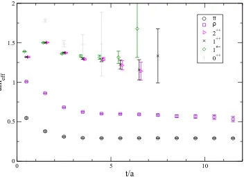
2++ 1++ 1+− 0++
Fig. 4. Effective masses for isovector mesons with 100 eigenvectors, time, colour, spin and space-even-odd dilution and 75 configurations.
4 Results
In this exploratory study, we use a data set consisting of 75 quenched config-urations atβ = 5.7 on a 123×24 lattice. We have used Wilson fermions with hopping parameter κ = 0.1675, corresponding to mπ/mρ = 0.50 [18]. The
100 lowest eigenvectors have been computed for each configuration, and noise vectors have been diluted in time, spin, colour and in space on an even/odd basis.
4.1 Isovector mesons
We have computed correlators for the pion, rho, the 1+−,0++,1++ and 2++ P-wave states, using spatially extended operators for the P-waves [17]. The quark fields were smeared with 10 levels of Jacobi smearing iterations. In cases where we use multiple operators for a single state, we have found some differences in the overlap depending on the spatial size of the operators where typically larger operators were favoured.
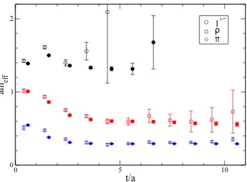
[image:12.612.96.448.71.326.2]0 5 10
t/a
0 1 2
am
eff
1+−
[image:13.612.94.448.67.328.2]ρ π
Fig. 5. Comparison of spectrum from all-to-all and point-to-all propagators. The open symbols are point-to-all, the closed symbols all-to-all with 100 eigenvectors and time, colour, spin and space-even-odd dilution.
We can also compare the results using our method with results using tradi-tional point-to-all propagators on the same number of configurations. These are shown in Fig. 5 for the pion, rho and 1+− P-wave. The P-wave was com-puted using point sources at 3 different spatial points in order to construct the derivative operator. While the improved signal for the pion may not jus-tify the additional computational expense, it is clear that for the rho meson and in particular the P-wave the reduction in noise is very significant with all-to-all propagators. This is particularly important if only a limited number of configurations is available, which will be the case for light, dynamical full QCD configurations. In the case of P-waves (as well as hybrids, and of course isoscalar mesons) all-to-all propagators may be the only way of obtaining any acceptable signal at all.
4.1.1 Effect of dilution
0 5 10 15 20 25
# inversions per timeslice
0 5 10
∆
C
___
C
(t=3) (%)
Nev= 0 Nev= 100
[image:14.612.98.445.70.320.2]π
Fig. 6. Demonstration of the effect of dilution on the statistical errors as a function of dilution, for the pion. The squares denote the errors obtained using only noise vectors, while the diamonds are errors obtained using the hybrid method.
N independent noise samples per time slice. This curve is given by
σ2N =
σ2 1 −σg2
N +σ
2
g, (40)
where σg is the gauge noise, i.e. the statistical uncertainty resulting from
having a finite number of gauge configurations. We have assumed that the gauge noise is given by the errors from the hybrid method with our highest dilution level, σg =σ24hyb. We see in all cases studied here that dilution always works better than accumulating an equivalent number of independent noise samples. A closer inspection reveals that the errors fall off like 1/N rather than the naive 1/√N. This is in addition to the exponential gain due to time dilution.
4.1.2 Effect of eigenvectors
0 5 10 15 20 25
# inversions per timeslice
0 5 10 15 20 25 30
∆
C
___
C
(t=3) (%)
Nev= 0 Nev= 100
10 20
1 2 3
[image:15.612.95.445.79.325.2]ρ
Fig. 7. Demonstration of the effect of dilution on the statistical errors as a function of dilution, for theρ. The squares denote the relative errors on the correlator on time slice 3 obtained using only noise vectors, while the diamonds are errors obtained using the hybrid method. The solid line is the expected behaviour of the errors from accumulating an equivalent number of independent (time-diluted) noise samples. The inset shows the relative errors from the hybrid method in more detail.
0 5 10 15 20 25
# inversions per timeslice
0 50 100 150
∆
C
___
C
(t=3) (%)
Nev= 0 Nev= 100
10 20
5 10
1
+− [image:15.612.96.446.443.688.2]0 5 10 15 20 25
# inversions per timeslice
0 50 100
∆
C
___
C
(t=3) (%)
Nev= 0 Nev= 100
[image:16.612.92.446.69.600.2]1
++Fig. 9. As Fig. 7, for the 1++ P-wave.
0 5 10 15 20 25
# inversions per timeslice
0 10 20 30 40 50
∆
C
___
C
(t=3) (%)
Nev= 0 Nev= 100
[image:16.612.96.445.70.326.2]2
++Fig. 10. As Fig. 7, for the 2++ P-wave.
and lattice spacing used, and the non-chiral action and coarse lattices used in this exploratory study would be unlikely to yield valuable information for more realistic simulations.
0 5 10
t/a
0 0.5 1
am
eff
N ev= 50 N
ev= 100
Hybrid method N
[image:17.612.95.449.67.325.2]ev= 100
Fig. 11. The ρ effective masses from the 50 and 100 lowest eigenvectors alone, and from the hybrid method with 100 eigenvectors. The corresponding figure for the pion is shown in Fig. 3.
hybrid method with 100 eigenvectors. We observe a dramatic decrease in the relative error of the estimated correlator when the lowest 100 eigenvectors are used. The exception is the pion, where the errors remain constant at about 5% (from our 75 configurations) regardless of dilution and eigenvectors. We interpret this as an effect of the pathologies of Wilson fermions on coarse lattices with light quarks, where the large fluctuations of the lowest eigenmode affect the pion in particular.
The insets of Figs 7 and 8 show the errors for the hybrid method in more detail as a function of dilution, for the ρ meson and 1+− P-wave. The gauge noise level appears to be reached somewhere between dilution levels 6 (colour and space even/odd) and 12 (colour and spin), although a slight downward trend may still be observed at Ndil = 24 for the P-waves. It is interesting to note that fractional error reached for the vector meson is much smaller than the pseudoscalar (for this rough action).
4.2 Isoscalar mesons
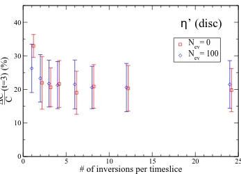
0 5 10 15 20 25
# of inversions per timeslice
0 10 20 30 40
∆
C
___
C
(t=3) (%)
Nev= 0 Nev= 100
[image:18.612.98.445.65.315.2]η
’ (disc)
Fig. 12. As fig. 7, for the disconnected piece of the isoscalar correlation function.
total uncertainty is saturated by the gauge noise almost immediately. This is not surprising on this coarse lattice with a non-chiral action, but it gives confidence that a good signal can be obtained from a proper action.
4.3 Static–light mesons
The benefit of using all-to-all propagators is particularly evident in simulations of heavy-light mesons in the static limit. Using a single point propagator for the light quark means that the source and sink of the static-light correlator are restricted to a single spatial lattice site. All-to-all propagators allow us to place source and sink operators at each spatial site on the lattice, yielding a dramatic increase in statistics. The application of all-to-all propagators to the static-light spectrum has previously been examined in Refs. [6,19].
The mesons considered in the previous sections are classified according to their
JP C quantum numbers. Here, however, the mesons contain non-degenerate
quarks and charge conjugation is no longer a symmetry of the meson. Also, static-light mesons which differ only in the spin of the static quark are de-generate. Therefore, in the static limit, we find a single S-wave channel and two distinct P-wave channels. We label theseJP
ℓ where Jℓ is the total angular
momentum of the light degrees of freedom. The S-wave is then 12− and the P-wave channels are 12+ and 32+.
parame-0 5 10
t/a
0.5 1 1.5
am
eff
1/2+ 3/2+ 1/2−
Fig. 13. Effective masses for the static–light S-wave and P-waves, calculated using 100 eigenvectors and time, colour, spin and space-even-odd dilution.
ters are the same as for the isovector mesons shown in Fig. 4 and, once again, we have used extended operators for the P-waves. We obtain excellent signals in each channel and, as Fig. 14 shows, we are able to determine the P-wave ground-state energies to within 1% accuracy. Physically, the 32+ is expected to be heavier than the 12+ [19] but, given the coarseness of the lattice and the actions used, we do not expect our results to be physically meaningful.
The results were obtained using the variational method with five operators differing by the Jacobi smearing parameters of the light quark. This is a very simple way of extending the basis operators to get a better overlap with the ground state and for identifying excited states. As Fig. 15 shows, we find clear signals for the first and second excited states of the S-wave. We can also resolve signals for the first excited states of both P-waves.
Figures 16–18 show the relative errors for the static–light meson correlators as a function of dilution level. For the 1
2 −
and 3 2 +
the errors are already saturated by the gauge noise with time dilution alone, while for the 1
2 +
[image:19.612.96.448.67.324.2]0 1 2 3 4 5 6 7 8
t/a
0 0.1 0.2 0.3
a(M
1/2
+
−
M
3/2
+
)
[image:20.612.94.448.65.319.2]aδM=0.122(1)
Fig. 14. The energy-difference between the static–light P-wave ground states, with the line denoting the best fit.
0 5 10
t/a
0.6 0.8 1 1.2 1.4 1.6
am
eff
ground state
1st excited state
2ndexcited state
Fig. 15. Effective masses for the three lowest-lying states of the static–light S-wave.
5 Conclusions
[image:20.612.93.448.362.619.2]0 5 10 15 20 25
# inversions per timeslice
0 0.5 1
∆
C
___
C
(t=5) (%)
[image:21.612.96.444.80.331.2]1/2
−Fig. 16. Demonstration of the effect of dilution on the error-bars as a function of dilution, for the static–light S-wave, with 100 eigenvectors. The solid line is the expected behaviour of the errors from accumulating an equivalent number of inde-pendent, time-diluted noise samples.
0 5 10 15 20 25
# inversions per timeslice
0.5 1 1.5 2 2.5
∆
C
___
C
(t=5) (%)
1/2
+ [image:21.612.98.445.430.679.2]0 5 10 15 20 25
# inversions per timeslice
0 0.5 1
∆
C
___
C
(t=5) (%)
[image:22.612.95.445.65.313.2]3/2
+Fig. 18. As fig. 6, for the static–light 32+ P-wave.
in a gauge configuration, which considering the cost to generate full QCD con-figurations may be of crucial importance. They are also a necessary ingredient in flavour-singlet physics and in computing fermionic thermodynamic quanti-ties.
All-to-all propagators have a further advantage over point propagators in that operator construction is considerably simplified: the operators are constructed in a natural way from local fields, and extended operators used in variational methods may be employed at no additional cost.
We have presented evidence that diluting stochastic estimators in time, colour, spin or other variables gives less variance than traditional noisy estimators. This is not unexpected, since dilution will yield the exact all-to-all propagator in a finite number of iterations. More work is needed to determine the optimal dilution path for different observables, although the simplest choices (colour, space even/odd, and to some extent spin dilution) are often sufficient to reach the gauge noise level for the ensemble sizes considered here.
The hybrid method allows one to extract the important physics from low-lying eigenmodes and combine this with a noisy correction in a natural way. This may be implemented so that the user can be blind to the details of the dilution and eigenvector list.
statistics.
Although we have focused on (mainly isovector) mesons in this study, the method is also straightforwardly applicable to baryons and to thermodynamic quantities (condensates and susceptibilities). Work on flavour singlets and thermodynamic observables is currently in progress.
Acknowledgments
This work was funded by an IRCSET award SC/03/393Y and the IITAC PRTLI initiative.
References
[1] K. Bitar et al., Nucl. Phys. B313 (1989) 348.
[2] Y. Kuramashi et al., Phys. Rev. Lett. 71 (1993) 2387.
[3] S.J. Dong and K.F. Liu, Phys. Lett. B328 (1994) 130 [hep-lat/9308015].
[4] G.M. de Divitiis et al., Phys. Lett. B382 (1996) 393 [hep-lat/9603020].
[5] SESAM, N. Eicker et al., Phys. Lett. B389 (1996) 720 [hep-lat/9608040].
[6] UKQCD, C. Michael and J. Peisa, Phys. Rev. D58 (1998) 034506 [hep-lat/9802015].
[7] UKQCD, C. McNeile and C. Michael, Phys. Rev. D63 (2001) 114503 [hep-lat/0010019].
[8] W. Wilcox, Numerical Challenges in Lattice Gauge Theories, edited by A. Frommer et al., , Lecture Notes in Computational Science and Engineering Vol. 15, pp. 127–141, Berlin, 2000, Springer [hep-lat/9911013].
[9] H. Neff et al., Phys. Rev. D64 (2001) 114509 [hep-lat/0106016].
[10] A. Duncan and E. Eichten, Phys. Rev. D65 (2002) 114502 [hep-lat/0112028].
[11] MILC, T. DeGrand and U.M. Heller, Phys. Rev. D65 (2002) 114501 [hep-lat/0202001].
[12] SESAM, G.S. Bali et al., hep-lat/0505012.
[13] M.J. Peardon, Nucl. Phys. Proc. Suppl. 106 (2002) 3 [hep-lat/0201003].
[14] TrinLat, A. O’Cais et al., hep-lat/0409069.
[16] L. Venkataraman and G. Kilcup, hep-lat/9711006.
[17] UKQCD, P. Lacock et al., Phys. Rev. D54 (1996) 6997 [hep-lat/9605025].
[18] F. Butler et al., Nucl. Phys. B430 (1994) 179 [hep-lat/9405003].