The Role of Verification in Computer Modelling: A Case Study in Solidification Processing

THE ROLE OF VERIFICATION IN COMPUTER MODELLING: A CASE STUDY IN SOLIDIFICATION PROCESSING

R.P. Mooney¹ and S.McFadden1

1. Department of Mechanical and Manufacturing Engineering, Trinity College Dublin, Dublin 2, Ireland.

Corresponding author: [email protected]

ABSTRACT

Computer modelling has become an important aspect of engineering science and technology. Bespoke computer models are routinely under development and are often applied to specific manufacturing and materials processes. Solidification processes (casting, for example) is no exception and significant numbers of modelling approaches for solidification are available in the literature. The roles of verification and validation in model development for any physical process ought to be clear, but owing to practicalities, it can be difficult to fully verify or fully validate a computer model to a specific requirement. Hence, the terms verification and validation are routinely interchanged or are misconstrued to mean the same thing. This paper outlines a verification study for a Bridgman Furnace Front Tracking Model (BFFTM) of solidification. A formal order verification procedure was applied which showed that the prediction from the computer model converged, in agreement, with an analytical model of the same process. Hence, verification of the BFFTM was achieved.

KEYWORDS: modelling, verification, solidification

1.

Manufacturing, like so many other engineering disciplines, has enjoyed the benefits of computer modelling. Once confidence in a particular computer model is achieved, the benefits of applying the computer model will include improved prediction of results and improved understanding of the underpinning physical processes involved. When engineers have at their disposal a powerful and well-understood predictive computer model it allows for improved (and cheaper) design and planning of a particular activity—design iteration with a virtual model of the process generally takes less time and costs less than physical design iteration with an experimental rig. (However, it is not suggested that virtual modelling completely replace physical testing.)

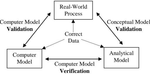
Verification and Validation are terms that are often used in computer modelling. There are differences in opinion in the literature regarding the definition and usage of each term, but for the purposes of this article, we have adopted the approach outlined in several sources such as Sargent [1], Roache [2], and Banaszek [3], among others. Figure 1 gives a flowchart that shows how verification and validation are related to the real-world process and their mathematical descriptions.

Figure 1: Verification and Validation Schematic

Verification applies to computer modelling and analytical modelling only. Specifically, it refers to the process by which one demonstrates that a discretised partial differential equation (PDE) code correctly solves its governing equations. This process involves comparison of numerically simulated results with a known analytical (exact) solution to the PDE. The computer model is verified if this comparison is adequately close (to some acceptable level). In other words, the numerical model accurately solves the equations that constitute the mathematical model. Typically, a successful verification is achieved by the removal of coding errors and by refining the model discretisation scheme to an acceptable level.

Validation refers to applicability of the model (numerical or mathematical) to the physical system under investigation. In computer modelling, validation involves comparison of numerically simulated data with measured experimental data. Validation is carried out to confirm that the PDE being solved is representative of the real system being modelled. Strictly speaking, validation is only achieved within the range of experimental conditions investigated.

Boehm [4] and Blottner [5] define verification as “solving the equations right”, and validation as “solving the right equations”.

Verification and validation are often difficult. Validation relies on the ability to observe or unobtrusively measure some distinct parameter that the computer model simulates. This may not always be the case as some parameter may be unmeasurable. Hence, different levels or subset definitions of validation have been proposed [1]. Verification is often difficult because the analytical (exact) solution to the mathematical model may be difficult or impossible to obtain. Typically, an analytical (or closed-form) solution to a PDE may only be available for a simple case with simplifying assumptions applied.

Real-World Process

Analytical Model Computer

Model

Conceptual Model Validation Computer Model

Validation

Computer Model Verification

This paper uses a case study in modelling to demonstrate a formal order verification procedure [2] applied to a computer model of a Bridgman Furnace Front Tracking Model (BFFTM) of solidification [6].

Fortunately, in this case, an analytical solution for the mathematical problem exists.

1.1 Verification Procedure

The verification procedure is illustrated by the flowchart in Figure 2. First, the theoretical order of accuracy of the model is determined via the governing equations and the finite difference scheme used in the model. Second, a test problem is designed. Third, an exact solution to the PDE of interest must be found. Following this, the code is run at two different grid resolutions. The results from these simulations are then used to calculate the observed order of accuracy,

p. If the observed order of accuracy does not match the theoretical order of accuracy then coding errors exist.

Figure 2. Code verification procedure, adapted from Knupp and Salari [7].

The local numerical errors NEilocal can be calculated by their difference at

each discrete position;

.

num i exact i local

i

T

T

NE









,

1







i

num i exact i global

T

T

N

NE

where N is the total number of control volume or mesh nodes. The observed order of accuracy for the numerical scheme, p, is calculated using the global numerical error at two grid resolutions x1 and x2, as follows,

.

ln

ln

2 1

2 1





































x

x

NE

NE

p

global x global

x

(3)

1.2 The Bridgman Furnace – The Test Problem

A schematic of a Bridgman furnace is shown in Figure 2. The furnace is made up of three zones: a hot zone with heater held at a temperature, TH, having a

heat transfer coefficient with the sample, hH; an insulated adiabatic zone of

length, LA; and a cold zone with heater held at a temperature, TC, having a heat

transfer coefficient with the sample, hC. Normally, the hot zone is held at a

temperature above the melting temperature of the sample material, while the cold zone is held at a temperature below the melting temperature. A cylindrical sample with radius, r, is contained in a hollow thin-walled crucible. The crucible and sample are translated at a fixed velocity, v, through the furnace. A solidification interface is formed at some position in the adiabatic zone where the temperature is equal to the material melting temperature, TM. In steady state solidification the

position of the interface and the temperature profile are stationary relative to the furnace which is fixed to ground.

Figure 2: Schematic of a Bridgman furnace.

and pulling velocity, v, and it is a simple dimensional exercise to show that the product of G and v gives the cooling rate of the solidification process as the sample passes through the liquid-solid phase change.

2.

In order to proceed with the exercise, two models of the same process are required, namely, a computer model, which is to be verified, and a mathematical model (with an exact analytical solution). Both models are based on the PDE given below, which is a 1-dimensional heat equation with a latent heat or source term, an advection term, and a term for the circumferential heat exchange).







T

T



E

,

A

P

h

x

T

C

v

x

T

k

x

T

C

t

C H p

p

_





































_

_

Further details on this equation are available in Mooney et al. [7]. The first term on the left hand side will reduce to zero for the steady state problem.

2.1 Computer Model – Bridgman Furnace Front Tracking Model

The BFFTM is described elsewhere [6,8]. The BFFTM is based on a 1-dimensional discretisation of equation 1 using a Finite Difference Control Volume method. A marker is used to determine the location of the solidification front. This marker is governed by a growth law, thereby allowing the model to determine local equilibrium at the solidification front rather than global equilibrium across the entire domain [9].

2.2 Mathematical Model

The corresponding mathematical model for this test problem is given under steady state conditions as





0

,

2

















T

T

Bi

X

T

Pe

X

T

where Pe is the Péclet number and Bi is the Biot number—as given by equations (6) and (7).

k

rv

C

Pe





k

r

h

Bi



(7)

,

0

0 _X

S S X L L f

X

T

k

X

T

k

L













where Lf is the rate of latent heat of liberated at the interface per unit area;

,

f L

f

v

H

L







and Hf is the latent heat of fusion of the material per unit mass.

3.

The verification exercise was performed using basic data for pure titanium; however, the material selection choice is inconsequential for the purposes of verification. The verification could have proceeded with any pure material. Simulations were carried out at four different grid resolutions starting at x = 0.8 mm and reducing the resolution by a factor of two until x = 0.1 mm. In each case the resulting steady state temperature profile from the numerical model was compared to the analytical solution and the global numerical error was calculated. The observed order of accuracy was then calculated by comparing results over two consecutive grid refinements. Table 1 shows a summary the results obtained.

Table 1: Results from the verification procedure.

Simulation run

Grid resolution,

x [mm]

Global numerical error, NEglobal [°C]

Theoretical order of Accuracy

Observed order of Accuracy, p

#1 0.8 2.11

1 0.61 #2 0.4 1.38

1 1.07 #3 0.2 0.66

1 0.98 #4 0.1 0.33

4. DISCUSSION

The results show that as the grid resolution was reduced from 0.8 mm to 0.1 mm the global numerical error also reduced. The theoretical order of accuracy, constant throughout the procedure, was deduced from the equations to be unity. The observed order of accuracy, p, which was calculated by comparing results at various grid resolutions, was shown to tend towards unity especially at the finer grid resolutions. Hence, the observed order of accuracy converged to the theoretical order of accuracy, as required.

prediction for simulation #3, i.e., 0.02% of the domain size, and 0.02 mm for simulation #4, i.e., 0.01% of the domain size.

5. CONCLUSION

The distinction between verification and validation in computer modelling was reviewed in this manuscript. A validation exercise relates the suitability of a model to simulate the intended real-world process. Verification is the process of checking if a numerical solution is correctly implemented and so is required before a validation can be achieved. This paper demonstrated a formal verification procedure for a benchmark manufacturing process, namely, solidification processing in a Bridgman furnace.

References

[1] R.G. Sargent, Verification, Validation, and Accreditation of Simulation Models, in J.A Jones, R.R. Barton, K. Kang and P.A. Fishwick (eds)

proceedings of the 2000 Winter Simulation conference, Orlando, 2000, 50– 58

[2] P.J. Roache, Verification of Codes and Calculations, AIAA Journal. Vol. 36 (1998) 696–702

[3] J. Banaszek, Credibility analysis of computer simulation of complex heat transfer problems, in Nowak, A.J., Białecki, R., Węcel, G. (eds) Eurotherm Seminar 82 Numerical Heat Transfer, Gliwice-Cracow, 2005, 141–63. [4] B.W. Boehm, Software Engineering Economics, Prentice-Hall (1981) [5] F.G. Blottner, Accurate Navier-Stokes results for the hypersonic flow over a

spherical nosetip, Journal of Spacecraft and Rockets. Vol 27 (1990) 113–122 [6] R.P. Mooney, S. McFadden, M. Rebow, D.J. Browne, A Front Tracking Model for Transient Solidification of Al–7wt%Si in a Bridgman Furnace,

Tranaction of the Indian Institute of Metals. Vol. 65 (2012) 527–530

[7] P. Knupp, K. Salari, Verification of Computer Codes in Computational Science and Engineering, CRC Press (2003)

[8] R.P Mooney, S. McFadden, Z. Gabalcová, J. Lapin, An experimental-numerical method for estimating heat transfer in a Bridgman furnace,

Applied Thermal Engineering, Vol.67 (2014) 61–71

[9] R.P. Mooney, S. McFadden, Order Verification of a Bridgman Furnace Front Tracking Model in Steady State, Simulation Modelling Practice and Theory,

accepted for publication.

[10] R.J. Naumann, An analytical approach to thermal modeling of bridgman-type crystal growth: I. One-dimensional analysis, Journal of Crystal Growth.