Munich Personal RePEc Archive
Gravity for Outsourcing: an Application
with Input-Output Dataset.
de Mello-Sampayo, Felipa
ISCTE-IUL
2014
Online at
https://mpra.ub.uni-muenchen.de/59843/
Gravity for Outsourcing: an Application with Input-Output
Dataset
∗Felipa de Mello-Sampayo
Abstract
This paper examines the impact of gravity on outsourcing. We derive a gravity equation from the classical spatial supply problem in which firms purchase some of their inputs from other firms paying the required transport costs. We also allow for different levels of productivity of the firms and build a gravity equation from entropy maximiza-tion. Even if the gravity equations look similar, we show that their underlying structures are different. In general terms, countries are viewed as competing with each other for interaction. The competing destinations gravity model represents a step forward in the recognition of interdependencies in spatial choice. Thus, we include a variable to explain the spatial structure of outsourcing countries in a geographical system. We find much stronger support for the gravity equation derived from the probabilistic input demand function than for the deterministic gravity model. The model shows that outsourcing is carried out mostly because of factor cost differentials and technological differences, but that distance and the gravity of other countries adversely affect trade in intermediate goods and services.
JEL Classification: C21; F12; F23; R15
Keywords: Outsourcing, Gravity Model, Trade, MNEs, Poisson regression
Postal address: ISCTE-IUL, Department of Economics, Av. For¸cas Armadas, 1649–026, Lisbon, Portugal.
∗Financial support from Funda¸c˜ao para a Ciˆencia e Tecnologia, under UNIDE-BRU is gratefully
1
Introduction
One of the distinctive characteristics of the current globalization process is the emergence of global value chains. Within global value chains and international production networks, not only are final goods traded internationally, but also intermediate goods (parts, components, and semi-finished goods) and services. Exports of final goods are no longer an appropriate indicator of the competitiveness of countries, as following the emergence of global value chains, final goods increasingly include a large proportion of intermediate goods that have been imported into the country. This trend greatly alters the economic relationships between countries and casts increasing doubt on empirical indicators such as trade and FDI, which are traditionally used to measure globalization.
Trade flows have been analyzed using gravity equations. Although first put forward as an intuitive explanation of bilateral trade flows, the gravity model has more recently acquired a range of micro-founded theoretical bases. These approaches are important to policy researchers because they affect the data, specification, and econometric technique used to estimate the gravity model. Use of a theoretically-grounded gravity model can lead to substantially different results and interpretations from those obtained via an intuitive for-mulation, and high quality policy research and advice increasingly needs to be based on a rig-orously established methodology. The literature provides a variety of theoretically-grounded gravity models (Anderson, 1979, Bergstrand, 1985, Anderson and van Wincoop, 2003, 2004, Anderson, 2010, Baier and Bergstrand, 2001, 2002, 2007, 2009, Eaton and Kortum, 2002, Evenett and Keller, 2002, Feenstra, 2004, Bergstrand, Egger and Larch, 2007). It is only recently that gravity models have been applied to the empirical analysis of cross-border long-term capital flows or cross-border multinational activities (Brainard, 1997, Braconier, Norb¨ack and Urban, 2005, Egger and Pfaffermayr, 2004, de Mello-Sampayo, 2009, Kleinert and Toubal, 2010). Chaney (2008) and Helpman, Melitz and Rubinstein (2008) develop gravity-like equations based on underlying models of trade in which firms are heterogeneous in productivity. Although there are important differences among the exact forms of grav-ity produced by these models, they all retain some fundamental similarities with the basic model.
problem in which firms purchase some of their inputs from other firms paying the required transport costs. There are many reasons why the classical specification is not realized in practice. These include imperfect information available to the firms, differences in tech-nology between the so-called identical firms, and differences in strategic objectives. In the second model, we allow for different levels of productivity of the firms and build a gravity equation from entropy maximization. Even if the gravity equations look similar, we show that their underlying structures are different.
Anderson and van Wincoop (2003) demonstrate that the traditional gravity equation is mis-specified and coefficient estimates are likely biased owing to omission of nonlinear mul-tilateral resistance terms. These mulmul-tilateral resistance variables capture the dependence of trade flows between trading countries on trade costs across all possible trading suppliers. Fol-lowing Anderson and van Wincoop’s (2003) seminal paper addressing omitted variables bias in the gravity equation, we include a variable to explain the spatial structure of outsourcing countries in a geographical system. In general terms, countries are viewed as competing with each other for interaction. One possible measure of destination competition is the com-petition factor, a composite variable that attempts to capture the gravity of the competing destinations (de Mello-Sampayo, 2009). The competing destinations gravity model repre-sents a step forward in recognition of interdependencies in spatial choice (Fotheringham, 1983a,b, Thorsen and Gitlesen, 1998). Its main difference from the classic version stems from the fact that a competition factor encompassing the ability of third destinations to attract interaction flows is included as a dampening factor to inputs flowing to any potential destination.
loss in degrees of freedom imposed by the fixed effects estimator. The method of Anderson and Yotov (2010) avoids the approximation error observed by Baier and Bergstrand (2009). The empirical application of the gravity model is fundamentally about inferring trade costs (Anderson and van Wincoop, 2004, Anderson, 2010). There have been several notable advances in modeling and inferring trade costs, namely dealing with the implications of zeros in the bilateral trade flow data. One view of zeros is that they stand for flows too small to report. Interpreting zeros in this way, it is legitimate to drop the zero observations from estimation because there is no economic significance to the zeros relative to the non-zero observations. Alternatively, zeros may be explained by high fixed costs of export. If no firm is productive enough to make incurring the fixed cost of exporting profitable, then zero trade results (Helpman et al., 2008). One way of dealing with this problem is to use the sample selection correction introduced by Heckman (1979). The selection effect determines which markets are active and also determines a volume effect due to productivity heterogeneity among firms whereby markets that are active have a greater or lesser number of firms active depending on the same selection mechanism. In the presence of heteroskedastic errors, Santos-Silva and Tenreyro (2006) point out that inconsistent estimation arises from the usual econometric gravity practice using logarithmic transformation and estimated with Ordinary Least Squares (OLS). Since the data have many zeros, the disturbance term must have a substantial mass at very small values, violating the normal distribution assumption. They propose instead to model the disturbance term as generated from a Poisson distribution, leading to estimation with a Poisson Pseudo-Maximum Likelihood (PPML) technique. Their results show that PPML leads to smaller estimates of trade costs compared to OLS.
We derive the gravity equation from two different models, using the derived gravity equations to discriminate between the deterministic gravity model and the probabilistic gravity model. In order to discriminate between the gravity equations, we need intermediate sales data with variation in factor endowments and in market size. We use an input-output dataset for the the United States, Europe, Japan, Brazil, Russia, India, and China, for 2005. Input-output tables offer complementary insights into the globalization of value chains as they provide information on the value of intermediate goods and services that have been imported from outside the country. A key advantage of I-O tables is that they classify goods according to their use, as an input into another sector’s production or as final demand, instead of classification schemes that divide goods into intermediate and other categories based on their descriptive characteristics. Another key advantage of I-O tables is that they also include information on inputs in services sectors, so that the outsourcing activities can be monitored.
analytical framework proposed in this paper.
The paper is structured as follows. In the following sections we derive the theoretical explanations for the gravity equation applied to outsourcing. In Section 2 we derive a gravity equation from the classic spatial supply optimization problem. In Section 3 we depart from the assumption of symmetric firms, and present a heterogeneity-based gravity equation based on the entropy maximization problem. In Section 4 we discuss the estimation strategy, and present the estimation results in Section 5. We conclude in Section 6.
2
The Deterministic Gravity Model
The economy consists of two sectors of activity. Final good firms, which employ labor and a set of inputs to produce a unique consumption good; intermediate good firms which have monopoly power over the production of its input. The technology to produce final goods is represented by the following production function:
Y =L1y−α
n
Z
0
xαvdv, (1)
wherexv is the quantity of the inputv,nis the measure of inputs available,Ly is the labor,
and α gives the intensity of the preference for inputs’ variety, 0 < α < 1. The additive separability of the function implies that the inputs are different (imperfect substitutes), although they are neither intrinsically better nor worse. The marginal product of each input is decreasing but there are constant returns to the number of inputs, n, which can be regarded as the level of technical knowledge.
Let wy denote the salary in the final sector, and pv be the price of the variety v of
intermediate input. The final product is the numeraire. The representative firm in the competitive final sector maximizes profits, given by:
Πy =L1y−α n
Z
0
xαvdv−wyLy−
n
Z
0
pvxvdv. (2)
The first-order conditions provide the following factor demand functions:
pv =αL1y−αxvα−1, v ∈[0, n], (3)
and
wy = (1−α)L−yα
Z n
0
xαv. (4)
The marginal cost of producing any inputs is equal to wv. The profit of intermediate firms
is given by:
Maximize Equation (5) subject to the demand function as given by Equation (3), to get the price and the quantity, respectively:
pv=
wv
α , (6)
and
xv =α
1 1−αLyp
1
α−1
v . (7)
Consider the world economy is divided into final good producing countries i,i= 1,2, . . . , I, and input suppliers’ countries, j= 1,2, . . . , J. However, some countries might produce both the final goods and intermediates. Let X = Pvijxvij be defined as the total number of
input interactions, and we wish to model the interaction pattern between countries, i.e. xijs
the flow of inputvbetween countryj andi. Thus, final good firms located in countryibuy some of their inputs from countryj, paying the required transport costs. When a firm ships inputs from country j to country i, it must send τij >1 units in order for a single unit to
arrive:
Pvij =pvjτij, (8)
where pvj is the price of the input v produced in country j. Thus, the price of the input
is increased by distance costs of the iceberg type. When inputs are produced in the home countryi,i=j, the firm continues paying transport costs, τii>1.
Countryi’s import of input v from county j is given by:
xvij =Pvijxvj, (9)
wherexvj is the quantity of the inputv produced in countryj. Substituting Equations (6),
(7), and (8) into Equation (9), we obtain the countryi’s demand for varietyv from country
j:
xvij = (wvjτij)
α
α−1 αLyi. (10)
In equilibrium, all intermediate firms in a given country-sector are symmetrical in terms of marginal cost, sales, price, etc. Using the measure of firms active in country j, nj, we can
write total sectoral imports as:
xij = n
X
v
xvij =nj(wjτij)
α
α−1αLyi. (11)
This equation of bilateral intermediates’ trade can be transformed into a gravity equation for intermediates. It contains home country’s demand characteristics and supply characteristics of the outsource country. Following Redding and Venables (2003), we refer to njw
α α−1
j as
outsource country’s supply capacity and denote it by sj. We call αLyi home country i’s
market capacity and denote it by mi. Equation (11) can be written as xij =sj(τij)
The standard form of the gravity model as presented in Equation (11) contains an in-dependence from the irrelevant alternatives (IIA) property: the ratio of flows to any two destinations is independent of any other destination (Fotheringham, 1984). The IIA axiom may be modified to reflect interdependencies in spatial choice. If these interdependencies are introduced into the gravity model, the ratios of predicted flows from remaining suppliers will be affected by the choice of a particular supplier region (Fotheringham, 1984). Problems with the IIA principle occur in other choice modeling contexts, see for example Anderson and van Wincoop (2003) on trade and de Mello-Sampayo (2009) on FDI location choices.
In general terms, destination areas are viewed as competing with each other for interac-tion. One possible measure of destination competition is the competition factor, a composite variable that attempts to capture the gravity of the competing destinations. Country i’s total expenditure on inputs from country j′scompetitors,Di, is given by:
Di =αLyi
X
k6=j
nk(wkτik)
α
α−1 . (12)
Solving Equation (12) forαLy and substituting the result into the sectoral imports Equation
(11) gives:
xij=
nj(wj)
α α−1 (τij)
α α−1 P
k6=jnk(wkτik)
α α−1
Di. (13)
Equation (13) can be written as xij = sj(τij)
α
α−1 micj, where sj = njw
α α−1
j stands for
country j’s supply capacity, mi =Di gives country i’s market capacity sinceDi converges
asymptotically, in the limit, to the total demand of country i, andcj =Pk=6 jnk(wkτik)
α α−1
is a composite variable that captures the gravity of the competing destinations.
There are many reasons why the above classic solution is not realized in practice. These include imperfect information available to the firms, differences in technology between the so-called identical firms, and differences in strategic objectives. In fact, if for a certain base period we have enough commodity flow data to evaluate the actual realized profits by substitution of the observed flows into Equation (2), the resulting total profits can never be greater than the results of the classic deterministic solution, and will often be considerably less. Thus, if we are interested in projecting the state of the spatial supply system at a future point in time, we formulate and fit a model to reproduce the observed total profits, ΠObs, which at the same time has the asymptotic property that it converges in the limit to the classic solution of Equation (2).
3
The Probabilistic Gravity Model
Consider the observed stock of inputs XObs
vj of each input v in country j, as well as the
unknown usage Xvi =Pjxvij of each input v for the output of the final good in country
we would not identify the firms with individual shipments, as above, but would look at the receiving firms, i.e. country i’s total expenditure on inputs, Di. Thus, we consider the
number of waysS that distinct observed shipments from region j,XObs
vj , can be allocated in
groups xvij to the countryiand the number of ways the Xvi shipments arriving at country
ican be arbitrarily allocated to the Di distinct receiver firms:
S =
Q
vj
XObs vj !
Q
i
xvij!
Q
vi
DXvi
i . (14)
The log-linearized form of Equation (14) is determined, the Stirling approximation1 applied, and constant terms omitted, then the entropy S comes out as:
S=−X
vij
xvij[ln(
xvij
Di
)−1]. (15)
Now, assuming that we are going to reproduce the observed input flowsXObs
vj of each inputv
out of each countryj, which the firms at countryicompete for, an extra calibration feature not available to the classic deterministic model, the following sum constraints should be applied:
X
i
xirs =XvjObs. (16)
The maximization of Equation (15) is constrained by the model flows being induced to con-form with certain aggregate base period quantities. If we have the observed total production
YObs based on the observed sales in all countries i, the following production constraint is
applied:
X
i
Yi =YObs, (17)
whereYiis given by Equation (1). Inputs that are imported from countryjinto countryiare
subject to melting-iceberg transport costs. Reproducing the observed average generalized cost of travel τObs, yields:
X
vij
xvijτij =XτObs. (18)
Now assume there is a potential measurecj that measures the relative competitive position
of country j, i.e. the competing destinations’ potential relative to countryj. Reproducing the observed average generalized competing destinations’ potentialcObs, yields:
X
vij
xvijcvj =XcObs. (19)
1The Stirling approximation is given byx! =x(lnx
Maximize Equation (15) under the row sum constraints in Equation (16) with Langrange multiplierλ, and the key behavioral constraint Equation (17) with multiplierβ,and Equation (18) with multiplier ϕ, and Equation (19) with multiplier δ, making use of Equation (7), and imposing that the predicted total interaction flow leaving each origin should equal the observed value, i.e. XObs
vj =
P
ixirs to obtain:
xvij =
XvjObsDieβ
nj wvj
α +ϕτij+δcvj
P
iDieβ
nj wvj
α +ϕτij+δcvj
. (20)
which has a similar form to a conditional logit model (probabilistic input demand function) and where β,ϕand δ are parameters to be estimated. The parameters β and ϕreflect the perception of outsource countries’ attractiveness and distance as determinants of interactions by the firms of countryi. The balance of total flows are ensured byXObs
vj /
P
iFieλ
nj wvj α +βτij. The variablenjwvj
α represents the country j’s competitiveness for outsourcing. We expectβ
to be positive, indicating that as the competitiveness of countryj’s outsource increase, the volume of interactions between iandj increase. Conversely, we expectϕto be negative: as the economic distance between country iand region j increases, the volume of interaction between them decreases.
In general terms, destination areas are viewed as competing with each other for interac-tion and when a variable measuring such competiinterac-tion is included in the gravity framework, the resulting interaction models are known as competing destinations models (Fothering-ham, 1983a). One possible measure of destination competition is the competition factor, a composite variable that seeks to capture the gravity of the competing destinations (see de Mello-Sampayo, 2009):
cvj =
X
k6=j
βnkwvk
α /ϕτik, (21)
wherecvj is the sum, weighted by economic distance, of all other outsource countries’
char-acteristics (except country j) in supplying inputs to i. The variable nkwvk
α represents the
competitiveness of outsource countryk;τik represents the economic distance between
coun-tryiand outsource countryk;βandϕare defined as in the gravity model given by Equation (20). Often they are set to one in the competition formulation (Roy, 2004). A negative value of δ in Equation (20) demonstrates the presence of competition or congestion forces. The above model structure clearly represents a great step forward in recognition of interdepen-dencies in spatial choice. Its main difference from the classic version stems from the fact that a competition factor encompassing the ability of third destinations to attract interaction flows is included as a dampening factor to inputs flowing to any potential destination.
avj =
X
k6=i,j
βnkwvk
α /ϕτjk, (22)
where avj represents the accessibility of country j in relation to all other countries. The
higher the competitiveness of country k, and the closer these countries are to j (i.e., the smaller isτjk), the lower is the flow expected fromjtoisince there is a spatial concentration
of opportunities in the neighborhood of j. In this situation the access measure avj models
competition effects since it will be high but the flow low, so that this type of accessibility has a negative impact on flows if several countries with large masses are close to each other. Alternatively, it may model agglomeration effects if the higher the competitiveness of country
k, and the closer these countries are to j, the higher is the flow expected from j to isince there is a spatial concentration of opportunities in the neighborhood of j. In this situation the access measure avj will be high and the flow high, so that this type of “accessibility”
has a positive impact on flows if several areas with large masses are close to each other. Comparing the sectoral imports Equation (13) and the conditional logit model as given by Equation (20), we observe that though they look similar, there are differences. The main difference is the aggregation level of Equation (13). There is aggregation bias due to sectorally varying trade costs and sectorally varying elasticities of trade with respect to trade costs (Anderson and van Wincoop, 2004, Anderson and Yotov, 2010). The second aggregation problem is specification bias because GDP, is a value added concept with a variable relationship to gross trade flows. Much recent attention to the vertical disintegration of production and its international aspect emphasizes the variable intertemporal relationship of gross trade to GDP and its variation across countries is also significant. Disaggregation and use of the appropriate sectoral output and expenditure variables fixes both problems (Anderson, 2010). The other difference relates to the restrictions on the parameters of the models. The gravity equation derived from the deterministic model as given by Equation (13) imposes restrictions on the parameters of the country’s supply capacity and market capacity to be one, the parameter on distance to be negative and, on competition factor to be minus one. This suggests that the probabilistic gravity model is more general.
4
Data and Estimation Strategy
We use an input-output dataset that has been taken from the Institute of Developing Economies, Japan External Trade Organization, IDE-JETRO, for the the United States, Europe, Japan, Brazil, Russia, India, and China, for 2005. The Input-Output Database shows transactions, wherever possible, in industry-by-industry symmetric tables at basic prices. The non-energy imported intermediate inputs’ dataset are disaggregated into six sectors: agriculture, livestock, forestry and fishery; Manufacturing; Electricity, gas and wa-ter supply; Construction; Trade and transport; and Services.
Data on the Technological environment and dissemination of technology are from Profils Institutionnels database of CEPII. Distances come from GeoDist database of CEPII. We use bilateral distance in kilometers between the two capitals, and distance weighted by the share of the city in the overall country’s population developed by Head and Mayer (2002). The labor costs proxies considered here are the wage per capita by economic activity. The descriptive statistics are shown in the Appendix.
We start estimating the gravity equation for imports of intermediate inputs as derived from the deterministic model, but disaggregating the dependent variable, the labor cost, and the competition factor at the industry level, and using fixed effects. The log-linearized form of Equation (13) yields the following gravity equation:
ln (xvij) =γ0+γ1ln (nj) +γ2ln (wvj) +γ3ln (τij) +γ4ln (Di) +γ4ln (cvj) +λv+λi+λj+εvij,
(23) where γ0 is a constant, γ2 = γ3 = αα−1, i denotes the importing country, j the exporting
country, xvij denotes the log of intermediate imports of inputv from countryj to country
i, τij is the distance between country i and country j measured in kilometers, Di is the
importing country’s real GDP, nj is the exporting country’s level of technical knowledge,
wvj is the exporting country’s labor costs, cvj is the competition factor or an index that
yields the gravity faced by countryj from all other countryi’s trading partners;λv denotes
industry effects, λi the importer country effects,λj the exporter country effects, andεvij is
an error term.
The labor cost parameter γ2 and distance parameterγ3 are negative, since 0< α <1.
The structural gravity equation implies a constraint on the estimates of parameter γ1 and γ4. They must equal one, and γ5 equals minus one. It is straightforward to test whether
these constraints hold in the empirical analysis.
Then, we estimate the probabilistic gravity model. We follow Santos-Silva and Tenreyro (2006) and estimate a Poisson model pseudomaximum likelihood. The conditional logit model as given by Equation (20) for the matrix of input flows,xvij, from countryjto country
i may be specified in terms of Poisson sampling (Guimaraes, Figueiredo and Woodward, 2003):
xvij ∼Poisson(µvij), i= 1,2, . . . ,7; j= 1,2, . . . ,7, v = 1,2, ...,6 (24)
where the Poisson mean is predicted by:
b
µvij =Di :nj :wvj:τij :cvj. (25)
In Equations (24) and (25), all variables are identical to Equation (23); with the exception of the dependent variable. The dependent variable, xvij, is the number of inputs vimported
from country j into countryi.
be biased because log-linearization of the dependent variable changes the property of the error term, which becomes correlated with the explanatory variables in the presence of het-eroskedasticity. In addition, log-linearization is incompatible with the existence of zeros in affiliates sales data. As emphasized by Helpman et al. (2008) and Baltagi, Egger and Pfaf-fermayr (2014), omitting the zero-valued observations leads to a nonrandom sample that can result in biased or inconsistent estimates.
5
Results
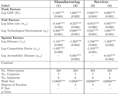
The results are presented for two separate cases. In the first case, presented in Table 1, we use the full set of non-energy industries. Each observation corresponds to a reporting country–partner–sector combination. The second part of our empirical approach, presented in Table 2, uses data for individual industries, taking the manufacturing and services sectors separately. As in manufacturing, the outsourcing of intermediates in services has been increasing in the last decade. While outsourcing of intermediates, just like the trade of final products, has traditionally been occurring in manufacturing industries, the emergence of global value chains increasingly stretches out to services sectors.
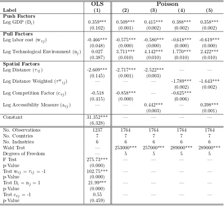
(Insert table 1 here)
Table 1 is arranged into two main sections. The first is composed of column (1), which corresponds to the estimation of the gravity equation as given by Equation (23), and the other composed of columns (2) to (5), which correspond to the gravity equation as given by Equations (24) and (25). All specifications include a full set of industry, country i, and country j fixed effects. The robust standard errors have been computed as described by Wooldridge (1999). Columns (3) and (5) show the results for the estimation of the probabilistic gravity equation when the competition factor, cvj, in columns (2) and (4) is
replaced by the accessibility measure variable, avj, to test the competition-agglomeration
hypothesis. In a robustness check, columns (4) and (5) show the results for the estimation of the probabilistic gravity equation when the bilateral distance in kilometers between the two capitals used in columns (2) and (3) is replaced by distance weighted by the share of the city in the country’s overall population. In Table 1, for every Poisson model, according to the Wald test the overall significance of the regressors is not rejected at the 1% significance level. The deterministic model is also not rejected with a highly significant F-test.
one, and that the coefficients on distance and labor costs are equal and negative. The re-strictions on the coefficients on countryi’s GDP and country j’s technological environment being equal to unity and that the coefficients on distance between countries and countryj’s labor costs being equal are rejected at the 1% level of significance. Still, the constraint that the coefficient on the competition composite variable that captures the competition faced by countryj in outsourcing to countryito be equal to minus one is supported by the data. Regarding the estimation of the probabilistic gravity model, the coefficient estimates all have the correct signs and are significant as observed in columns (2) to (5). Overall, the em-pirical results give more support to the probabilistic gravity model, since all variables have the expected sign and are statistically significant. The estimates of the gravity model under both spatial patterns’ characterizations suggest, as expected, a positive and significant coef-ficient for countryi’s GDP, a positive and significant coefficient for countryj’s technological environment, and a negative and significant coefficient for the countryj’s labor costs, which suggests that comparative advantages play an important role in outsourcing. With regard to the variables that make up the spatial factors in the model, namely distance in kilometers between the two capitals used in columns (2) and (3) and distance weighted by the share of the city in the country’s overall population used in columns (4) and (5), the results show the importance of distance in outsourcing. With respect to the variables that characterize the geographical pattern in the model, competition factor and accessibility measure, the estimated negative and significant effect of the competition factor on intermediates’ imports reflects the fact that the higher the competitiveness and the better localized the concurrent outsourcing countries, the less outsourcing one expects to occur to a particular country. The result by which the accessibility measure affects outsourcing positively is explained by the fact that the more accessible a outsourcing country is to its competitors raises its outsourcing opportunities. However, the remarkable feature of the present results is the strong impact of the competition factor. The relevance of such a result in the present context is that, by highlighting the importance of the gravity of alternative countries on input flows, it lends overwhelming support to the analytical framework proposed in this paper.
(Insert table 2 here)
reflecting the generally greater complexity of technology-intensive goods as they typically require a broad range of inputs.
6
Conclusion
Gravity has long been one of the most successful empirical models in economics. Incorpo-rating the theoretical foundations of gravity into recent practice has led to a richer and more accurate estimation and interpretation of the spatial relationships described by gravity. We derive competing destinations gravity equations explaining outsourcing from two very dif-ferent models to argue that the success of the gravity equation in empirical studies results from the fact that it can be derived from various models. In both models firms fragment their production process in order to benefit from countries’ comparative advantages. First, we derive a gravity equation from the classic spatial supply problem in which firms purchase some of their inputs from other firms paying the required transport costs. Then, we allow for different levels of productivity of the firms and build a gravity equation from entropy maximization. Even if the gravity equations look similar, we show that their underlying structures are different. The derived gravity equation additionally entails a competition fac-tor, a variable to explain the spatial structure of outsourcing countries in the geographical system under consideration.
References
Anderson, J. E. (1979), ‘A theoretical foundation for the gravity equation.’,American Eco-nomic Review69, 106–116.
Anderson, J. E. (2010), The gravity model., Technical report, NBER Working Paper No. 16576.
Anderson, J. E. and van Wincoop, E. (2003), ‘Gravity with gravitas: a solution to the border puzzle’,American Economic Review93, 170–192.
Anderson, J. E. and van Wincoop, E. (2004), ‘Trade costs.’,Journal of Economic Literature
42, 691–751.
Anderson, J. E. and Yotov, Y. V. (2010), ‘The changing incidence of geography.’,American Economic Review100, 2157–86.
Baier, S. L. and Bergstrand, J. H. (2001), ‘The growth of world trade: tariffs, transport costs, and income similarity.’,Journal of International Economics53, 1—-27.
Baier, S. L. and Bergstrand, J. H. (2002), On the endogeneity of international trade flows and free trade agreements., Technical report, University of Notre Dame, Available from
http://www.nd.edu/ jbergstr/W orkingPapers/EndogeneityAug2002.pdf.
Baier, S. L. and Bergstrand, J. H. (2007), ‘Do free trade agreements actually increase mem-bers’ international trade?’,Journal of International Economics71, 72––95.
Baier, S. L. and Bergstrand, J. H. (2009), ‘Bonus vetus OLS: A simple method for approx-imating international trade cost effects using the gravity equation.’, Journal of Interna-tional Economics77, 77–85.
Baltagi, B. H., Egger, P. and Pfaffermayr, M. (2014), Panel data gravity models of interna-tional trade., Technical report, CESIFO Working Paper No. 4616.
Bergstrand, J. H. (1985), ‘The gravity equation in international trade: some microeconomic foundations and empirical evidence.’,Review of Economics and Statistics 67, 474–481.
Bergstrand, J. H., Egger, P. and Larch, M. (2007), Gravity redux: Struc-tural estimation of gravity equations with asymmetric bilateral trade costs., Technical report, University of Notre Dame, Available from http :
//www.nd.edu/ jbergstr/W orkingPapers/GravityReduxOctober2007.pdf.
Braconier, H., Norb¨ack, P.-J. and Urban, D. (2005), ‘Reconciling the evidence of the knowl-edge capital model.’,Review of International Economics 13, 770–786.
Chaney, T. (2008), ‘Distorted gravity: The intensive and extensive margins of international trade.’,American Economic Review98, 1707–1721.
de Mello-Sampayo, F. (2009), ‘Competing-destinations gravity model: an application to the geographic distribution of FDI’,Applied Economics 41, 2237–2253.
Eaton, J. and Kortum, S. (2002), ‘Technology, geography, and trade.’, Econometrica
70, 1741–1779.
Egger, P. and Pfaffermayr, M. (2004), ‘Distance, trade and FDI: A SUR.’,Journal of Applied Econometrics19, 227–246.
Evenett, S. and Keller, W. (2002), ‘On theories explaining the success of the gravity equa-tion.’,Journal of Political Economy110, 281–316.
Feenstra, R. (2004), Advanced International Trade: Theory and Evidence., Princeton Uni-versity Press, Princeton, NJ.
Fotheringham, A. S. (1983a), ‘A new set of spatial-interaction models: The theory of com-peting destinations’,Environment and Planning A 15, 15–36.
Fotheringham, A. S. (1983b), ‘Some theoretical aspects of destination choice and their rele-vance for production-constraint gravity models’,Environment and Planning A 15, 1121– 32.
Fotheringham, A. S. (1984), ‘Spatial flows and spatial patterns’, Environment and Planning A16, 529–42.
Grossman, G. M. and Rossi-Hansberg, E. (2006a), The rise of offshoring: It’s not wine for cloth anymore, The New Economic Geography: Effects and Policy Implications, Federal Reserve Bank of Kansas City.
Grossman, G. M. and Rossi-Hansberg, E. (2006b), Trading tasks: A simple theory of off-shoring, Working Paper 12721, National Bureau of Economic Research.
Guimaraes, P., Figueiredo, O. and Woodward, D. (2003), ‘A tractable approach to the firm location decision problem.’,Review of Economics and Statistics 85, 201–04.
Head, K. and Mayer, T. (2002), Illusory border effects: Distance mismeasurement inflates estimates of home bias in trade., Technical report, CEPII, Working Paper No 2002-01.
Heckman, J. (1979), ‘Sample selection bias as a specification error.’, Econometrica47, 153– 61.
Kleinert, J. and Toubal, F. (2010), ‘Gravity for FDI.’, Review of International Economics
18, 1–13.
Redding, S. J. and Venables, A. J. (2003), ‘South-East-Asian export performance: External market access and internal market supply.’, Journal of the Japanese and International Economies17, 404–441.
Roy, J. R. (2004), Spatial Interaction Modelling: A regional Science Context, Springer– Verlag, Berlin Heidelberg New York.
Santos-Silva, J. and Tenreyro, S. (2006), ‘The log of gravity.’,The Review of Economics and Statistics88, 641–58.
Thorsen, I. and Gitlesen, J. P. (1998), ‘Empirical evaluation of alternative model specifica-tions to predict commuting flows’,Journal of Regional Science 38, 272–92.
Data
Descriptive Statistics
Variables Mean Std. Dev. Min. Max.
Dependent Variable
Input Imports (in millions) 17.7 143 0 3431 Log Input Imports 10.885 4.671 -4.605 21.956 Push Factors
Log GDP 28.626 1.177 27.36 30.26 Demand for inputs 21 521.11 5 049.17 10 180 42 220 Pull Factors
Log Labor cost 0 2.746 -8.08 8.08 Log Technological Environment 0 0.388 -0.92 0.92 Spatial Factors
Tables to be Included in Main Text
Table 1: Model Estimates
OLS Poisson
Label (1) (2) (3) (4) (5)
Push Factors
Log GDP (Di) 0.359*** 0.509*** 0.415*** 0.388*** 0.358***
(0.102) (0.001) (0.002) (0.002) (0.002)
Pull Factors
Log labor cost (wvj) -0.466*** -0.575*** -0.580*** -0.618*** -0.619***
(0.048) (0.000) (0.000) (0.000) (0.000) Log Technological Environment (nj) 0.027 3.711*** 4.142*** 1.770*** 2.422***
(0.387) (0.010) (0.010) (0.010) (0.010)
Spatial Factors
Log Distance (τij) -2.609*** -2.717*** -2.522*** — —
(0.145) (0.001) (0.003) Log Distance Weighted (τw
ij) — — — -1.789*** -1.643***
(0.002) (0.002) Log Competition Factor (cvj) -0.518 -0.858*** — -0.625***
(0.415) (0.000) (0.006)
Log Accessibility Measure (avj) — — 0.442*** — 0.398***
(0.003) (0.001) Constant 31.352*** — — — —
(6.328)
No. Observations 1237 1764 1764 1764 1764
No. Countries 7 7 7 7 7
No. Industries 6 6 6 6 6
Wald Test — 253000*** 257000*** 289000*** 289000*** Degrees of Freedom — 5 5 5 5
F Test 275.73*** — — — —
p-Value (0.000)
Test wvj =τij = -1 102.75*** — — — —
p-Value (0.000)
Test Di = nj = 1 21.99*** — — — —
p-Value (0.000)
Test cvj = -1 0.55 — — — —
p-Value (0.459)
Standard errors in parentheses. Robust Standard errors in parentheses in columns (3) and (4).
Table 2: Poisson Estimates for Manufacturing and Services Sectors
Manufacturing Services
Label (1) (2) (3) (4)
Push Factors
Log GDP (Di) 1.103*** 1.065*** 0.935*** 0.898***
(0.004) (0.002) (0.004) (0.001)
Pull Factors
Log labor cost (wvj) -0.448*** -0.357*** -0.074*** -0.007***
(0.002) (0.000) (0.000) (0.000) Log Technological Environment (nj) 0.262*** 0.980*** 0.947*** 1.695***
(0.001) (0.001) (0.001) (0.001)
Spatial Factors
Log Distance (τij) -1.181*** -1.202*** -1.556*** -1.202***
(0.003) (0.002) (0.004) (0.002) Log Competition Factor (cvj) -1.037*** — -1.319***
(0.000) (0.001)
Log Accessibility Measure (avj) — 0.364*** — 0.443***
(0.003) (0.004)
Constant — — — —
No. Observations 294 294 294 294
No. Countries 7 7 7 7
No. Industries 6 6 6 6
Wald Test 113000*** 113000*** 422000*** 422000*** Degrees of Freedom 5 5 5 5
F Test — — — —
p-Value