External Balances, Trade Flows and Financial Conditions

Munich Personal RePEc Archive

External Balances, Trade Flows and

Financial Conditions

Evans, Martin

Department of Economics, Georgetown University

1 May 2014

Online at

https://mpra.ub.uni-muenchen.de/55644/

External Balances, Trade Flows and

Financial Conditions

Martin D. D. Evans

Department of Economics, Georgetown University.

30th April 2014

This paper studies how changing expectations concerning future trade and financial conditions

are reflected in international external positions. In the absence of Ponzi schemes and arbitrage

opportunities, the net foreign asset position of any country must, as a matter of theory, equal

the expected present discounted value of future trade deficits, discounted at the cumulated world

stochastic discount factor (SDF) that prices all freely traded financial assets. I study the forecasting

implications of this theoretical link in 12 countries (Australia, Canada, China, France, Germany,

India, Italy, Japan, South Korea, Thailand, The United States and The United Kingdom) between

1970 and 2011. I find that variations in the external positions of most countries reflect changing

expectations about trade conditions far into the future. I also find the changing forecasts for the

future path of the world SDF is reflected in the dynamics of the U.S. external position.

Keywords: Global Imbalances, Foreign Asset Positions, Current Accounts, Trade Flows,

Interna-tional Asset Pricing

JEL Codes: F31, F32, F34

1

Introduction

This paper studies how changing expectations concerning future trade and financial conditions are

reflected in international external positions. Economic theory links a country’s net foreign asset

(NFA) position to agents’ expectations in a precise manner. In the absence of Ponzi schemes and

arbitrage opportunities, the NFA position of any country must equal the expected present discounted

value of future trade deficits, discounted at the cumulated world stochastic discount factor (SDF)

that prices all freely traded financial assets. In practice this means that changes in observed external

positions of countries across the world should reflect changing expectations about future trade flows

and future financial conditions represented by the world SDF, or some combination of the two. The

aim of this paper is to assess whether this is in fact the case. More specifically, the paper examines

the extent to which changing expectations about future trade and financial conditions are reflected

in the evolving external positions of 12 countries between 1970 and 2011.

To undertake this analysis, I present an new analytic framework that links each country’s current

NFA position to its current trade flows, expectations of future trade flows, and expectations

concern-ing future returns on foreign assets and liabilities in an environment without arbitrage opportunities

or Ponzi schemes. This framework incorporates several key features. First it accommodates the

secular increase in international trade flows and national gross asset/liability positions that have

taken place over the past 40 years. The secular growth in both trade flows and positions greatly

exceeds the growth in GDP on a global and country-by-country basis. Between 1970 and 2011,

the annual growth in trade and positions exceeds the growth in GDP by an average of 2.6 and 4.8

percent, respectively, across the countries studied.1

The second key feature concerns the identification of expected future returns. As a matter of

logic, expected future returns on a country’s asset and liability portfoliosmust affect the value of its

current NFA position, so pinning down these expectations is unavoidable when studying the drivers

of external positions. This is easily done in textbook models where the only internationally traded

asset is a risk free bond, but in the real world countries’ asset and liability portfolios comprise equity,

FDI, bonds and other securities, with risky and volatile returns. Pinning down the expected future

returns on these portfolios requires forecasts for the future returns on different securities and the

composition of the portfolios. To avoid these complications, I use no-arbitrage conditions to identify

the impact of expected future returns on NFA positions via forecasts of a single variable, the world

SDF. SDFs play a central role in modern finance theory (linking security prices and cash flows) and

appear in theoretical examinations of the determinants of NFA positions (see, e.g., Obstfeld, 2012).

A key step in my analysis is to show how the world SDF can be constructed from data on returns

and then used to pin down how expectations concerning future financial conditions are reflected in

external positions.

1

In the empirical analysis I study the external positions of 12 countries (Australia, Canada, China,

France, Germany, India, Italy, Japan, South Korea, Thailand, The United States and The United

Kingdom). I first show how the world SDF can be estimated from data on returns and discuss how

the estimates can be tested for specification errors. Next I turn to the identification of expectations.

In theory, external positions reflect expectations concerning the entire future paths of trade flows

and the world SDF, so we need to forecast over a wide range of horizons. For this purpose I use VARs

- a common approach in the literature following Campbell and Shiller (1987). I then compare the

present values of future trade flows and the world SDF based on the VAR forecasts with external

positions. If the actual expectations embedded in the external positions are well represented by

the VAR forecasts, the present values computed from those forecasts should be strongly correlated

with the external positions. This implication is borne out by my empirical findings using the VAR

forecasts for trade flows. Forecasts of trade flows far into the future are strongly correlated with

the external positions of 10 countries I study. Evidence on the role of expected future financial

conditions is less clear cut. While VAR forecasts for the world SDF suggest that there have been

persistent and sizable variations in the prospective future financial conditions that are relevant for

the determination of external positions, the forecasts are only weakly correlated with the positions of

many countries. One notable exception to this pattern is the United States, whose external position

is strongly correlated with the forecasts.

These findings add to a growing empirical and theoretical literature on international external

adjustment. The analytic framework I present is most closely related to the work of Gourinchas and

Rey (2007a). They derive an expression for a country’s NFA position from a “de-trended” version of

the consolidated budget constraint (that governs the evolution of a country’s NFA position from trade

flows and returns), that filters out the secular growth in trade flows and positions mentioned above.

Thus their analysis focuses on the “cyclical” variations in NFA positions, rather than the “total”

variations. Similarly, Corsetti and Konstantinou (2012) use the consolidated budget constraint to

derive an approximation to the current account that includes deterministic trends in the log ratios

of consumption, gross assets and gross liabilities to output to accommodate the long-term growth in

trade flows and positions (relative to GDP).2

On the theoretical side, Pavlova and Rigobon (2008),

Tille and van Wincoop (2010) and Devereux and Sutherland (2011) all study external adjustment in

open economy models with incomplete markets. In these models changing NFA positions primarily

reflect revisions in expected future trade flows and the world risk-free rate because the equilibrium

risk premia on foreign assets and liabilities are (approximately) constant. In contrast, the framework

I use allows for variations in the risk premia on assets and liabilities to also affect NFA positions.

My analysis also extends a related literature on international returns. Early papers in this

2

literature (Obstfeld and Rogoff, 2005; Lane and Milesi-Ferretti, 2005; Meissner and Taylor, 2006

and Gourinchas and Rey, 2007b) estimated that the return on U.S. foreign assets was on average

approximately three percent per year higher than the return on foreign liabilities. Subsequent papers

by Curcuru, Dvorak, and Warnock (2007) and Lane and Milesi-Ferretti (2009) argued that these

estimates were biased upward because of inaccuracies in data. In their recent survey, Gourinchas

and Rey (2013) show that alternative treatments of the data can produce average return differentials

between U.S. foreign assets and liabilities that differ by as much as 1.1 and 1.8 percent, depending

upon the sample period. My analysis shifts the focus away from average U.S. returns in two respects.

First, I use the returns on the assets and liabilities of major economies to estimate the world SDF.

Second I model how conditional expectations concerning the world SDF are related to external

positions. Gourinchas and Rey (2007a) also consider the short-horizon (one quarter) forecasting

power of the (cyclical) U.S. external position for returns on its NFA portfolio, and the return

differential between equity assets and liabilities. Here I study forecasting power of external positions

over longer horizons.

The remainder of the paper is structured as follows: Section 2 describes the data. I present the

analytic framework in Section 3. Section 4 describes how I estimate the world SDF and compute

long-horizon forecasts. I present the empirical results in Section 5. Section 6 concludes.

2

Data

I examine the external positions of 12 countries: the G7 (Canada, France, Germany, Italy, Japan,

the United States and the United Kingdom) together with Australia, China, India, South Korea

and Thailand. Data on each country’s foreign asset and liability portfolios and the returns on the

portfolios come from the databased constructed by Lane and Milesi-Ferretti (2001), updated in Lane

and Milesi-Ferretti (2009), available via the IMF’s International Financial Statistics database. These

data provide information on the market value of the foreign asset and liability portfolios at the end

of each year together with the returns on the portfolios from the end of one year to the next. A

detailed discussion of how these data series are constructed can be found in Lane and Milesi-Ferretti

(2009). I also use data on exports, imports and GDP for each country and data on the one year U.S.

T-bill rate, 10 year U.S. T-bond rate and U.S. inflation. All asset and liability positions, trade flows

and GDP levels are transformed into constant 2005 U.S. dollars using the prevailing exchange rates

and U.S. price deflator. All portfolio returns are similarly transformed into real U.S. returns. The

Lane and Milesi-Ferretti position data is constructed on an annual basis, so my analysis below is

conducted at an annual frequency.3

Although the span of individual data series differs from country

3

Milesi-to country, most of my analysis uses data spanning 1970-2011.

The Web Appendix describes the characteristics of the data in detail. Here I simply note several

prominent features. First, for many countries, variations in the ratios of net exports and NFA to

GDP are highly persistent. Second, the cross-country dispersion in the ratios has widened in the

last decade. Third, gross financial positions (i.e., the sum of foreign assets and liabilities) and trade

(i.e., the sum of export and imports) have grown much faster than GDP. Averaging across all the

countries, trade grew approximately 2.6 percent faster than GDP, while foreign asset and liability

positions grew 4.8 percent faster. There have also been swings in global trade growth and position

growth that are much larger than global business cycles. In light of these facts, the next section

presents an analytic framework that links a country’s current external position to prospective future

trade and financial conditions while accommodating the growth in trade and positions.

3

Analytic Framework

3.1

NFA Positions

The framework I develop contains three elements: (i) the consolidated budget constraint that links

a country’s foreign asset and liability positions to exports, imports and returns; (ii) a no-arbitrage

condition that restricts the behavior of returns; and (iii) a condition that rules out international

Ponzi schemes.

I begin with country’sn0

sconsolidated budget constraint:

F An,t F Ln,t=Xn,t Mn,t+Rn,tF An,tfa 1 Rn,tflF Ln,t 1. (1)

Here F An,t andF Ln,t denote the value of foreign assets and liabilities of country n at the end of

yeart, whileXn,t andMn,t represent the flow of exports and imports during yeart, all measured in

real terms (constant U.S. dollars). The gross real return on the foreign asset and liability portfolios

of country n between the end of years t 1 and t are denoted by Rfa

n,t and Rfln,t, respectively.

Equation (1) is no more than an accounting identity. It should hold true for any country provided

the underlying data on positions, trade flows and returns are accurate. Notice, also, thatF An,t and

F Ln,t represent the values of portfolios of assets and liabilities comprising equity, bond and FDI

holdings, and thatRfa

n,tandRfln,t, are the corresponding portfolio returns. These returns will generally

differ across countries in the same year because of cross-country differences in the composition of

asset and liability portfolios.

Next, I introduce the no-arbitrage condition. In a world where financial assets with the same

payoffs have the same prices and there are no restrictions on the construction of portfolios (such as

short sales constraints), there exists a positive random,Kt+1, such that

1 =E_t[Kt+1Ri_{t+1], (2)}

where Ri

t+1 is the (gross real) return on any freely traded asseti. Here Et[.] denotes expectations

conditioned on common period-tinformation. The variableKt+1is known as the stochastic discount

factor (SDF). This condition is very general. It does not rely on the preferences of investors, the

rationality of their expectations, or the completeness of financial markets.4

I assume that it applies

to the returns on every security in a country’s asset and liability portfolios, and so it also applies to

the returns on the portfolios themselves; i.e.

1 =E_t[Kt+1Rfa_n,t

+1] and 1 =Et[Kt+1Rfln,t+1]. (3)

Equations (1) and (3) enable me to derive a simple expression for a country’s NFA position.

First I multiply both sides of the budget constraint in (1) by the SDF and then take conditional

expectations. Applying the restrictions in (3) to the resulting expression and simplifying gives

E_{t[Kt+1N F An,t+1] =}E_{t[Kt+1(Xn,t+1 Mn,t+1)] +N F An,t. (4)}

Rearranging this expression and solving forward using the Law of Iterated Expectations we obtain

N F An,t =E_t

1

X

i=1

Dt+i(Mn,t+i Xn,t+i) +Et lim

i!1Dt+iN F An,t+i, (5)

whereDt+i =Qi_j=1Kt+j.

The last term on the right-hand-side on (5) identifies the expected present value of the country’s

NFA position as the horizon rises without limit using a discount factor determined by the world’s

SDF. To rule out Ponzi-schemes, I assume that

E_{t lim}

i!1Dt+iN F An,t+i= 0, (6)

for all countries n. For intuition, suppose a debtor country (i.e. a country with N F An,t < 0)

decides to simply roll over existing asset and liability positions while running zero future trade

balances. Under these circumstances, the country’s asset and liability portfolios evolve asF An,t+i=

Rfa

n,t+iF An,t+i 1 and F Ln,t+i =Rfln,t+iF Ln,t+i 1 for all i > 0. Since Et[Kt+1Xt+1] identifies the period tvalue of any periodt+1payoffXt+1, (4) implies that the value of claim to the country’s net

assets next period is just E_{t[Kt+1N F An,t+1] =}E_{t[Kt+1(Xn,t+1 Mn,t+1)] +N F An,t =N F An,t.}

This same reasoning applies in all future periods, i.e.,E_{t+i[Kt+i+1N F An,t+i+1] =N F An,t+i for all}

i >0, so the value of a claim to the foreign asset positionτ periods ahead isE_{t[Dt+τN F An,t+τ] =}

4

E_t[Dt+

τ 1Eτ 1[Kt+τN F An,t+τ]] = .. = N F An,t. Taking the limit as τ ! 1 gives N F An,t =

E_tlimi!1[Dt+iN F An,t+i]<0.Thus, the country’s current NFA position must be equal to the value

of a claim on rolling the asset and liability positions forward indefinitely into the future. Clearly

then, no country n can initiate a Ponzi scheme in period t when E_tlimi!1Dt+iN F An,t+i 0.

Moreover, sincePnN F An,t = 0by market clearing, if Etlimi!1Dt+iN F A˜n,t+i >0 for any one

country,˜n, then at least one other must be involved in a Ponzi scheme. Thus, the restriction in (6)

prevents any country from adopting a Ponzi scheme in periodt.

We can now identify the determinants of a country’s NFA position by combining (5) and the

no-Ponzi restriction (6):

N F An,t=E_t

1

X

i=1

Dt+i(Mn,t+i Xn,t+i). (7)

This equation states that in the absence of Ponzi schemes and arbitrage opportunities, the NFA

position of any countrynmust equal the expected present discounted value of future trade deficits,

discounted at the cumulated world SDF. As such, it describes the link between a country’s current

external position and the prospects for future trade flows (i.e. exports and imports) and future

financial conditions, represented by the future SDF’s inDt+i.

Several aspects of equation (7) deserve note. First, the equation is exact; i.e., it contains no

approximations. It must hold under the stated conditions for accurate NFA and trade data given

market expectations and the world SDF. Second, (7) holds whatever the composition of the country’s

asset and liability portfolios (i.e. whatever the fractions held in equity, bonds, etc.), and however

those fractions are determined (by optimal portfolio choice or some other method). Third, the

equation applies simultaneously across all countries. If news about prospective future financial

conditions anywhere change expectations concerning future world SDFs, it affects the NFA position

of all countries that anticipate running future trade surpluses or deficits. Equation (7) also takes

explicit account of risk. It states that a country’s NFA position is equal to the value of a claim to

the future stream of trade deficits in a world where those deficits are uncertain.

Finally, it is worth emphasizing that the expected future trade flows and SDF on the

right-hand-side of (7) represent the proximate determinants of the country’s NFA position. More fundamental

factors, such as demographic trends, fiscal policy or productivity growth, can only affect the NFA

position insofar as they impact on these expectations. Moreover, since the same SDF applies to all

countries, such fundamental factors can only account for cross-country differences in NFA positions

insofar as they impact prospective future trade flows.

3.2

Forecasting Implications

Equation (7) implies that all variations in a country’s NFA position reflect revisions in

forecasting power for future trade flows and/or SDFs. To investigate this empirical implication, we

must overcome two challenges: The first concerns the identification of the world SDF,Kt. Section

4 describes how I estimate Kt from data on returns. The second arises from fact that the present

value expression in (7) includes forecasts forDt+iMn,t+iandDt+iXn,t+i withDt+i =Q i

j=1Kt+j for

alli >0rather and forecast forMn,t+i,Xn,t+i andKt+iseparately. To meet this challenge, I use a

standard approximation.

To approximate the present value expression for each country’s NFA position, I first rewrite (7)

as

N F An,t =Mn,tE_t

1

X

i=1

exp⇣Pi_j=1∆mn,t+j+κt+j

⌘

Xn,tE_t

1

X

i=1

exp⇣Pi_j=1∆xn,t+j+κt+j

⌘

, (8)

whereκt= lnKtis the log SDF, and∆is the first-difference operator. (Throughout I use lowercase

letters to denote the natural log of a variable.) This transformation simply relates the NFA position

to the current levels of imports and exports and their future growth rates, ∆mn,t+i and ∆xn,t+i,

rather than the future levels of exports and imports shown in (7).

Next, I approximate to the two terms involving expectations. If δt is a random variable with

meanE_{[δt] =δ<0,then a first-order approximation toδt+j aroundδproduces}

E_t

1

X

i=1

exp⇣Pij=1δt+j

⌘

=E_{texp(δt+1) +}E_{texp(δt+1+δt+2) +...}

' ρ

1 ρ+ρEt(δt+1 δ) +ρ

2_E

t(δt+1 δ) +ρ3Et(δt+2 δ) +....

= ρ

1 ρ+

1 1 ρEt

1

X

i=1

ρi(δt+i δ), (9)

whereρ= exp(δ)<1.

To apply this approximation, I make two assumptions:

E_{[∆mn,t] =}E_{[∆xn,t] =g, and (A1)}

g+κ=δ<0, with E_[κt] =κ, (A2)

where E_{[.] denotes unconditional expectations. Under assumption A1 the mean growth rate for}

imports and exports are equal. This will be true of any economy on a balanced growth path and

appears consistent with the empirical evidence for the G7 countries. To interpret assumption A2,

note that in the steady state the log risk free ratersatisfies1 =E_{[exp(κt)] exp(r). Thusδ=g+κ}' g r 1₂V_{[κt], where}V_{[.]denotes the variance, so A2 will hold provided}V_{[κt]>2(g r).The mean}

growth rate for trade across the countries in the dataset is approximately 6.5 percent, which is well

above any reasonable estimate of the mean risk free rate of close to 1 percent. Clearly then, A2

bound is easily exceeded by estimates of the log SDF derived below.

Applying the approximation in (9) to the expectations terms in (8) and simplifying the result

gives

N F An,t= ρ

1 ρ(Mn,t Xn,t) +

1

2(1 ρ)(Mn,t+Xn,t)Et

1

X

i=1

ρi(∆mn,t+i ∆xn,t+i)

+ 1

1 ρ(Mn,t Xn,t)Et

1

X

i=1

ρi(∆τn,t+i g)

+ 1

1 ρ(Mn,t Xn,t)Et

1

X

i=1

ρi(κt+i κ), (10)

where ∆τn,t = 1₂(∆mn,t+∆xn,t). This expression identifies the three sets of factors determining

a country’s NFA position in a clear fashion. The first term on the right-hand-side identifies the

influence of the current trade balance. This would be the only factor determining the NFA

posi-tion in the stochastic steady state where import growth, export growth and the log SDF followed

i.i.d. processes because the terms involving expectations would equal zero. As such, this first term

identifies theatemporal influence of trade flows on the NFA position. The remaining terms on the

right-hand-side identify the intertemporal factors that were present in (7). In particular they make

clear how expectations concerning future trade flows and financial conditions, represented by the

world SDF, are (approximately) linked to a country’s current NFA position.

The influence of future trade and financial conditions on external positions can be further clarified

with a simply transformation of (10). For this purpose, I define countryn0

sexternal position by

N XAn,t= N F An,t

Mn,t+Xn,t

ρ

1 ρT Dn,t where T Dn,t=

Mn,t Xn,t Mn,t+Xn,t.

In words, the country’s NXA position is defined as the gap between its current NFA position and

the steady state present value of the future trade deficits, all normalized by the current volume of

international trade. Combining this definition with (10) gives

N XAn,t= ₂₍₁1_ρ)E_t

1

X

i=1

ρi₍

∆mn,t+i ∆xn,t+i) +₁1_ρT Dn,tEt 1

X

i=1

ρi₍

∆τn,t+i g)

+₁1_ρT Dn,tE_t

1

X

i=1

ρi(κt+i κ). (11)

Equation (11) provides us with the (approximate) link between a country’s current external

position and expectations concerning future trade flows and the SDF that forms the basis for the

empirical analysis below. For intuition, consider the effects of news that leads agents to revise

their forecasts for future trade deficits upwards. If there is no change in the expected future path

of the SDF, according to (7) there must be a rise in assets prices and/or a fall in liability prices

represented by the first two terms on the right-hand-side of (11).

The third term on the right-hand-side of (11) identifies how news concerning the future financial

conditions, as reflected by the SDF, affects a country’s external position. To illustrate the economic

intuition behind this term, consider the effect of news that lowers agents’ forecasts of the future

SDF but leaves their forecasts for future trade flows unchanged. Under these circumstances, (7)

shows that future trade deficits are discounted more heavily so the country’s current NFA position

is more closely tied to the value of a claim on its near-term deficits. Thus the NFA positions of

countries currently currently running trade deficits deteriorate while the NFA positions of those

running current trade surpluses improve. These variations in NFA are reflected one-to-one in NXA.

Equation (11) contains expectations conditioned on the common information set of agents in

period t, much of which is unavailable to researchers. To take this into account, let Φt denote a

subset of agents’ information attthat includesN XAn,tandT Dn,t. Taking expectations conditioned

onΦton both sides of (11) and applying the Law of Iterated Expectations, we find that

N XAn,t= 1

2PV(∆mn,t ∆xn,t) +T Dn,tPV(∆τn,t g) +T Dn,tPV(κt κ), (12)

where PV(υt) = ₁1_ρP 1

i=1ρiE[υt+i|Φt]. This equation takes the same form as (11) except the

agents’ expectations are replaced by expectations conditioned on Φt. Conditioning down in this

manner doesn’t affect the link between the country’s external position and the expectations because

information used by agents is effectively contained in Φtvia the presence ofN XAn,t andT Dn,t.

The implications of (12) for forecasting are straightforward. NXA should have forecasting power

for any stationary variable yt+k insofar as expected future values of that variable, E[yt+k|Φt], are

correlated with the present value terms on the right-hand side of (12). Suppose, for the sake of

illustration, thatytis independent of the trade flows and that the countryn’s long-run trade deficit

is equal to T Dn. Then a projection of yt+k on N XAn,t (i.e. a regression without an intercept)

would produce a projection coefficient equal to

E_{[yt+kN XAn,t]} E⇥_{N XA}2

n,t

⇤ = 1 1 ρE

"

T Dn,t 1

X

i=1

ρiE[(κt+i κ)|Φt]yt+k

E⇥_{N XA}2

n,t

⇤ #

= T Dn 1 ρ

1

X

i=1

ρi

CVhE_[κt+i|Φt],E_[yt+k|Φt]i E⇥_{N XA}2

n,t

⇤ .

where CV_{[., .] denotes the covariance. Notice that in this case the size of the coefficient depends}

on the both long run trade deficit, T Dn, and the covariance between the expectations ofyt+k and

κt+i over a range of horizonsi. In the empirical analysis below, I examine the forecasting power of N XAn,t for future trade flows withyt=∆mt ∆xt andyt=∆τt, and future financial conditions

withyt=κt at particular horizonsk. I also study the forecasting power ofN XAn,t for trade and

PV(∆mn,t ∆xn,t),PV(∆τn,t g)andPV(κt κ).

4

Empirical Methods

4.1

Estimating the World SDF

In a fully specified theoretical model of the world economy the world SDF would be identified from

the equilibrium conditions governing investors’ portfolio and savings decisions. Fortunately, for

our purposes, we can avoid such a complex undertaking. Instead, I adopt a “reverse-engineering”

approach in which I construct a specification for the SDF that explains the behavior of a set of

returns; the returns on the asset and liability portfolios for six of the G7 countries.5

This approach

is easy to implement and allows us to empirically examine how prospective future financial conditions

are reflected in external positions.

Leter_t+1 denote ak_⇥1 vector of log excess portfolio returns,eri

t+1 =rit+1 rttb+1, whererit+1 denotes the log return on portfolio i andrtb

t+1 is the log return on U.S. T-bills. I assume that the

log of the SDF is determined as

κt+1=a rtbt+1 b

0

(er_t+1 E[er_t+1]). (13)

This specification for the SDF contains k+ 1 parameters: the constant a and the k⇥1 vector

b. In the “reverse-engineering” approach values for these parameters are chosen to ensure that the

no-arbitrage conditions are satisfied for the specified SDF. More specifically, I find values foraand

bsuch that the portfolio returns for the asset and liability portfolios of the six G7 countries and the

U.S. T-bill rate all satisfy the no-arbitrage conditions.

Consider the condition for the i0

th portfolio return: 1 =E_{t[exp(κt+1+r}i

t+1)].Taking

uncondi-tional expectations we can rewrite this condition as

1 = E_{[exp(κt+1+rt}i_+1)]

' exp E_[κt+1+ri_t

+1] + 12V[κt+1+rti+1] . (14)

When the log returns are normally distributed the second line holds with equality because (13)

implies thatκt+1andrit+1are jointly normal. Otherwise, the second line includes an approximation error.

Next, I substituting for the log SDF from (13) in (14) and take logs. After some re-arrangement

this gives

a+E⇥_erti₊₁⇤₊1

2V

⇥

eri t+1

⇤

+1 2b

0

V_[er_t+1]b=CV⇥eri_t+1,er0_t+1⇤b. (15) 5

This equation must hold for the T-bill return (i.e., whenri

t+1=rtbt+1, or erit+1= 0) so

a+1 2b

0_V

[er_t+1]b= 0. (16)

Imposing this restriction on (15) gives

E⇥_erti₊₁⇤₊1

2V

⇥

eri t+1

⇤

=CV⇥_erti_+1,er0_t+1⇤b.

This equation holds for each of thek portfolio returns. So stacking thek equations we obtain

E_[er_t+1] +1

2Λ=Ωb, (17)

whereΩ=V_[er_t+1]andΛ is ak⇥1vector containing the leading diagonal of Ω.

Finally, we can solve (16) and (17). Substituting the solutions fora andb in (13) produces the

following expression for the log SDF:

κt+1= 1₂µ

0

Ω 1µ rtb

t+1 µ

0

Ω 1(er_t+1 E[er_t+1]). (18)

By construction, equation (18) identifies a specification for the log SDF such that the

uncondi-tional no-arbitrage condition,1 =E_[exp(κt+1+ri

t+1)], holds for thek log portfolio returns and the

return on U.S. T-bills. This specification would also satisfy the conditional no-arbitrage condition,

1 = E_{t[exp(κt+1+r}i

t+1)], if log returns were independently and identically distributed. However,

since this is not the case, we need to amend the specification to incorporate conditioning information.

Consider condition 1 = E_{t[exp(κt+1+r}i

t+1)]. Let ωt be a valid instrument known to market

participants in periodt. Multiplying both sides of the no-arbitrage condition byexp(ωt)and taking

unconditional expectations produces, after some re-arrangement

1 =Eh_exp(κt+1+ri,ω

t+1)

i

, (19)

where ri,ω

t+1 =rti+1+ωt lnE[exp(ωt)]. Notice that (19) takes the same form as (14) used in the

constructions of the log SDF in (18). The only difference is that (19) contains the adjusted log

return on portfolioi,ri,ω

t+1,rather than the unadjusted returnrti+1.This means that we can reverse

engineer a specification for the log SDF that incorporates the conditioning information if we add

adjusted log returns to the set of returns. Specifically, leteri,ωj

t+1 =rti+1 rtbt+1+ω

j

t lnE[exp(ω j t)]

denote the log excess adjusted return on portfolio iusing instrument ωjt. If ert+1 now represents a vector containing eri

t+1 and er

i,ωj

t+1, the log SDF identified in (18) will satisfy the non-arbitrage

condition

1 =Eh_exp(κt+1+ri_{t+1) ω}j_ti_,

Three aspects of this reverse engineering procedure deserve comment. First, equation (18) doesn’t

necessarily identify a unique SDF that satisfies the no-arbitrage conditions for a set of returns.

In-deed, we know as a matter of theory that many SDF exist when markets are incomplete. Rather

the specification in (18) identifiesone specification for the SDF that satisfies the no-arbitrage

condi-tions. Second, this reverse engineering approach makes no attempt to relate the SDF to underlying

macro factors. This complex task is unnecessary if our aim is simply to identify how prospective

future financial conditions affect external positions. The third aspect concerns the use of

instru-mental variables to control for conditioning information. In principle the conditional expectations

of market participants that appear in the no-arbitrage conditions equal expectations conditioned

on every instrumental variable in their information set. In practice, there is a limit to the number

of instruments we can incorporate into the log SDF specification. I chose instruments that have

forecasting power for log excess portfolio returns and I examine the robustness of my results to

alternative specifications for the log SDF based on different instrument choices.

I consider two empirical specifications for the log SDF. The first, denoted by κˆi

t, is estimated

from (18) without conditioning information. To assess whether the estimates satisfy the no-arbitrage

condition,1 =E_[exp(ˆκi

t+1+rit+1)|ω

j

t], I estimate regressions of the form:

exp(ˆκit+1+r

i

t+1) 1 =b1(f an,t f ln,t) +b2(xn,t mn,t) +vt+1, (20)

wherexn,t,mn,t,f an,t andf ln,t denote the logs of exports, imports, the value of foreign assets and

foreign liabilities, respectively, for countryn. Panel A of Table 1 reports the estimation results for

the log returns on the asset and liability portfolios. Notice that the log ratios of assets-to-liabilities

and export-to-imports are valid instruments so the estimates of b1 and b2 should be statistically

insignificant under the null of a correctly specified SDF. As Panel A shows, this is not the case

for the portfolio returns of four countries. The log asset-to-liability ratio has predictive power for

German, U.K. and U.S. returns, while the log export-to-import ratio has power for the returns on

Japanese assets.

In the light of these results, I incorporate conditioning information in my second specification

for the log SDF, denoted by ˆκii

t. Specifically, I now add the adjusted log return on U.S. assets,

ri,zt+1 =raus,t+1+ (f aus,t f lus,t) lnE[exp(f aus,t f lus,t)], whereraus,t+1 is the log return on U.S. assets, to the set of returns used to estimate the log SDF in (18). This specification incorporates

information concerning the future value of the SDF that is correlated with variations in the U.S.

NFA position. Thus, f aus,t f lus,t should not have forecasting power for exp(ˆκiit+1 +rit+1) 1 by construction. To check whether the other instruments retain their forecasting power, I then

re-estimate regression (20) withˆκii

t+1replacingκˆit+1. Panel B of Table 1 reports these regression results. In contrast to Panel A, none of theb1andb2coefficient estimates are statistically significant. Notice,

also, that theR2_{statistics are (in most cases) an order of magnitude smaller than their counterparts}

Table 1: Forecasting Returns

Asset Returns Liability Returns

b1 b2 R2 b1 b2 R2

A:κˆi

France 0.059 -0.210 -0.001 0.117 -0.205 0.003 Germany -0.428⇤

0.669 0.124 -0.442⇤⇤

0.594 0.129

Italy -1.031 2.436 0.135 -1.009 2.667⇤

0.143

Japan 0.299 2.304⇤⇤

0.098 0.327 2.374 0.106 United Kingdom -5.852⇤⇤

0.324 0.183 -5.843⇤⇤

0.437 0.177 United States -1.108⇤⇤

0.216 0.132 -1.059⇤⇤

0.252 0.115

B:ˆκii

France -0.188 -0.636 0.023 -0.116 -0.610 0.017 Germany -0.083 2.824 0.057 -0.091 2.862 0.059 Italy -0.653 -0.668 0.018 -0.653 -0.453 0.016

Japan 0.742 1.809 0.050 0.774 1.874 0.055

United Kingdom -4.595 2.237 0.052 -4.698 2.529 0.054 United States -0.229 0.515 0.022 -0.163 0.558 0.023

Notes: The table reports the OLS estimates of the regression (20) using theκitspecification for the log SDF in panel A and the κiit specification in panel B. “∗∗” and “∗” indicate statistical significance at the 5% and 10% levels, respectively. All regression estimated in annual data between 1971 and 2011.

meaningful fraction of the variation in exp(ˆκii

t+1+rit+1) 1. These findings appear robust to the

choice of estimation period and instruments. Re-estimating (20) over a sample period that ends in

2007 gives essentially the same results. I also find statistically insignificant coefficients in regressions

using ˆκii

t+1 as the log SDF when GDP growth rates and/or lagged returns are used as alternate

instruments.6

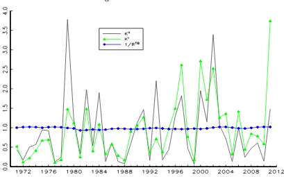
Figure 1 plots the two estimated SDFs,Kˆi

t= exp(ˆκit)andKˆtii= exp(ˆκiit), together with the inverse

of the real return on U.S. T-bills, 1/Rtb

t . In the special case where the expected excess portfolio

returns on assets and liabilities are zero, equation (18) implies that the SDF is equal to1/Rtb

t . Thus

differences between 1/Rtb

t and the estimated SDF’s arise because the SDFs must account for the

expected excess portfolio returns. As the plots clearly show, both estimates of the SDF are more

volatile than 1/Rtb

t . In fact, variations in the log return on U.S. T-bills contribute less than one

percent to the sample variance ofˆκi

tandˆκiit. Changes in U.S. T-bill returns do not appear to have an

economically significant impact on estimates of the SDF that “explain” returns on asset and liability

portfolios in major economies. The plots in Figure 1 also show that there are numerous episodes

where the estimated SDFs are well above one. Ex ante, the conditionally expected value of the SDF,

E_{tKt+1, identifies the value of a claim to one real dollar next period. So safe dollar assets sold at a}

premium during periods where these high values for the SDF were forecast ex ante.

6

Recall that specification forκ_tin (18) was derived using a log normal approximation to evaluate expected future returns. Based of these regression estimates, there is no evidence to suggest that the approximation is a significant source of specification error forκˆii

Figure 1: SDF Estimates

Notes: The figure plots two estimates of the world SDF,Kˆi

t= exp(ˆκit)andKˆtii= exp(ˆκiit), withκtdetermined in (18); and the inverse of the real return on U.S. T-bills,1/Rtb

t .

4.2

Estimating External Positions

The estimates of the log SDF, κˆii

t, allow us to pin down the discount rate ρ = exp(g+κ) used

in computing the NXA positions and the present value terms in equation (12). Recall that g is

the unconditional growth rate for exports and imports, which I estimate to be 0.064 from the

pooled average of import and export growth across countries. My estimate of κ computed from the average value of κˆii

t is -0.59. These estimates, denoted by gˆ and ˆκ, imply a discount rate of

ρ= exp(ˆg+ ˆκ) = 0.586. This is the value I use to construct the NXA measures of each country’s external position.

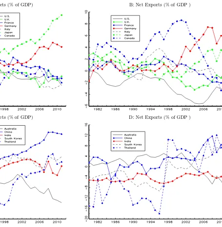
Figure 2 plots the NXA positions for each country in the dataset between 1980 and 2011. The

upper panel shows that the NXA positions for all but one of the G7 countries have remained between

±1 during the past 30 years. The one exception is the Japanese NXA position, which persistently

increased from 0.1 to 2.6 during the period. Variations in the NXA positions of countries outside

the G7 are generally larger. The plots in the lower panel of Figure 2 show large improvements in the

external positions of India and South Korea while Australia’s NXA position has remained largely

unchanged. It is also interesting to note that the steady improvement in the NXA position of China

in the last twenty years is not nearly as pronounced as the improvement in Japan’s position.7

Of

7

course the time series for the NXA positions reflect changes in NFA positions and trade deficits both

measured as a fraction of annual trade, N F An,t/(Mn,t+Xn,t)and (Mn,t Xn,t)/(Mn,t+Xn,t).

Plots for these variables are shown in the Web Appendix.

4.3

Long-Horizon Forecasts

In principle, variations in the NXA positions could reflect revisions in the expectations concerning

theentirepath for future imports, exports and the SDF. One way to investigate this possibility would

be to estimate regressions of realized present values; i.e.,Pk_i=1ρi_yt

+iforyt={∆mt ∆xt,∆τt g,

κt κ}, on N XAn,t for some finite horizon k. For example, with ρequal to 0.586, ρi < 0.01 for i >8, so a finite horizon of eight or nine years ought to be sufficient for this purpose. Unfortunately,

there are two well-known econometric problems with this approach. First, the coefficient estimates

may suffer from finite sample bias when the independent variables are persistent and predetermined

but not exogenous (see, e.g. Campbell and Yogo 2006). Second, the asymptotic distribution of the

estimates provides a poor approximation to the true distribution when the forecasting horizon is

long relative to the span of the sample (see, e.g. Mark, 1995), as it would be here with just a 40

year span.

To avoid these problems, I examine the relation between the NXA positions and P1

i=1ρiEˆtyt+i,

where the conditional expectationsEˆ_{tyt+iare computed from VARs. Specifically, let the vectorzt=}

[ yt, ., .. ]0

follow ap0

th. order VAR, which can be written in companion form asZt=AZt 1+Ut,

whereZt stacks thezt vectors appropriately. I estimate the present value foryt by

d

PV(yt) = 1 1 ρ

P1

i=1ρiEˆtyt+i= ₁ρ_ρı1Aˆ(I ρAˆ) 1Zt, (21) where ı1 is a vector that picks out the first row of Zt (i.e., yt = ı1Zt) and Aˆ denotes the

esti-mated companion matrix from the VAR. [The 1/(1 ρ) term is included for compatibility with the expression for the NXA position in equation (12)]. I compute present values for trade flows

where yt = ∆mn,t ∆xn,t or yt = ∆τn,t gˆ from VARs estimated country-by-country, and for

the log SDF with yt = κii

t ˆκ using a single world-wide specification. In all these calculations

ρ= exp(ˆg+ ˆκ) = 0.586.

I estimate the present value terms involving future trade flows (i.e., dPV(∆mn,t ∆xn,t) and

d

PV(∆τn,t ˆg)) from VARs that include the import-export growth differential∆mn,t ∆xn,t,trade

growth∆τn,t, and the log export-to-import ratioxn,t mn,t. Below I report results based on

first-order VARs estimated separately for each country,n; higher-order VARs give very similar results.

In addition, I considered estimates that includedN XAn,tand the log return on U.S. T-bills,rtb

t ,in

the VARs. The results presented below are robust with respect to the presence of these variables.8

I also use a VAR to compute the present value of the log SDF,dPV(ˆκii

t ˆκ). In this case the VAR

includesκˆii

t ˆκ, the log return on U.S. T-bills,rtbt ,the U.S. inflation rate, πtus,the spread between

the real yields on ten and one year U.S. T-bonds, sprus

t , and the average rate of real GDP growth

across the G7,∆yG7

t . In addition, I use the VAR to compute the present value of the log return on

8

U.S. T-bills, dPV(rtb

t rˆtb), where ˆrtb is the sample average ofrttb. Comparing dPV(ˆκiit ˆκ) with

d

PV(rtb

t rˆtb)proves useful when we examine how future financial conditional are reflected in the

NXA positions below.

5

Results

5.1

Forecasting Future Trade Flows

I begin by examining the short-horizon forecasting power of the NXA positions for trade flows. Panel

A of Table 2 reports slope coefficients, (heteroskedastic-consistent) standard errors andR2_statistics

from regressions ofyt+1on a constant andN XAn,t for each of the countries,n, over the full sample.

Columns I and II show estimates whereyt+1=∆mn,t+1 ∆xn,t+1 andyt+1= (∆τn,t+1 gˆ)T Dn,t are the forecast variables, respectively. These are the trade flows that appear in the present value

terms that determine the NXA position of countrynin equation (12). The estimates in column III

use the combination of trade flows that appears on the right-hand side of (12).

The results in Panel A of Table 2 show that information contained in the NXA positions

con-cerning future near-term trade flows differs considerably across countries. Among the G7, there is

no evidence that the NXA positions contain information about next year’s import-export growth

differential; none of the estimated slope coefficients are statistically significant at conventional

lev-els. By contrast, the NXA positions of China and South Korea appear to have reasonably strong

forecasting power for the differential. In both cases an increase in the NXA position forecasts a rise

in∆mn,t+1 ∆xn,t+1. Ceteris paribus, this is consistent with equation (12). For perspective on the size of coefficient estimates, the value of 10.3 implies that an increase in the Chinese NXA position

of 0.1 forecasts an increase in the growth differential of approximately one percent.

External positions have more widespread forecasting power for trade growth. Column II shows

that six slope coefficients are statistically significant at the one percent level. According to (12),

an increases in N XAn,t should, ceteris paribus, forecast a rise in trade growth for current deficit

countries and a fall in growth for surplus countries. This prediction is not borne out in five of

the six countries with significant coefficients. Finally, column III shows the forecasting power of

the NXA positions for the combined trade flows. Here there is very little evidence of any

short-horizon forecasting power. With the exception of China, none of the estimated slope coefficients are

statistically significant at the 10 percent level, and all theR2_{statistics are extremely small.}

All-in-all, the results in Panel A suggest that variations in prospective near-term trade flows play

no more than a minor role in driving variations in external positions. This doesn’t mean that future

trade flows are irrelevant. On the contrary, changes in external positions could reflect revisions in

expectations concerning the entire future path for trade flows (i.e. expectations well beyond the one

year horizon studied above). The results in Panel B of Table 2 allow us to examine this possibility.

Table 2: Forecasting Trade Flows

A: Short Horizon Forecasts

I II III

Forecast Variables ∆mn,t+1 ∆xn,t+1 ∆τn,t+1T Dn,t ∆mn,t+1 ∆xn,t+1+∆τn,t+1T Dn,t

coeff std R2 _{coeff std R}2 _{coeff std R}2

Canada 2.407 (1.811) 0.042 0.141 (0.186) 0.014 1.345 (0.885) 0.055 France -0.698 (0.646) 0.028 0.187⇤⇤⇤

(0.037) 0.386 -0.163 (0.323) 0.006 Germany 4.693 (3.818) 0.036 -0.802⇤⇤⇤

(0.280) 0.170 1.544 (1.991) 0.015 Italy 5.121 (3.683) 0.046 0.222 (0.236) 0.022 2.782 (1.848) 0.054 Japan 2.338 (1.947) 0.035 -0.210 (0.186) 0.031 0.959 (0.992) 0.023 United Kingdom 1.925 (1.806) 0.028 -0.419⇤⇤⇤

(0.096) 0.325 0.543 (0.883) 0.009 United States 0.877 (1.822) 0.006 -0.064 (0.199) 0.003 0.374 (0.919) 0.004

Australia -1.279 (4.853) 0.002 -0.308 (0.316) 0.023 -0.947 (2.374) 0.004

China 10.311⇤⇤

(4.929) 0.131 -0.920⇤⇤⇤

(0.351) 0.192 4.235⇤

(2.395) 0.097 India 0.518 (0.848) 0.009 -0.028 (0.099) 0.002 0.231 (0.457) 0.006 South Korea 2.603⇤⇤

(1.108) 0.124 -1.276⇤⇤⇤

(0.171) 0.588 0.025 (0.574) 0.000 Thailand 8.945⇤

(5.356) 0.065 -1.688⇤⇤⇤

(0.656) 0.142 2.785 (2.635) 0.027

B: Long-Horizon Forecasts

I II III

Forecast Variables PVd(∆mn,t ∆xn,t) PVd(∆τn,t g)T Dn,t dPV(∆mn,t ∆xn,t) +dPV(∆τn,t g)T Dn,t

coeff std R2 _{coeff std R}2 _{coeff std R}2

Canada 1.923 (1.244) 0.058 0.144 (0.386) 0.004 2.067 (1.478) 0.048 France -1.123⇤⇤⇤

(0.315) 0.246 -0.405⇤⇤⇤

(0.130) 0.199 -1.528⇤⇤⇤

(0.443) 0.234 Germany 7.750⇤⇤⇤

(1.530) 0.397 3.233⇤⇤⇤

(0.699) 0.354 10.982⇤⇤⇤

(2.213) 0.387 Italy 0.021 (2.105) 0.000 0.237 (0.814) 0.002 0.258 (2.908) 0.000

Japan 3.848⇤⇤⇤

(0.933) 0.304 0.607 (0.429) 0.049 4.455⇤⇤⇤

(1.309) 0.229 United Kingdom 5.004⇤⇤⇤

(0.725) 0.550 2.281⇤⇤⇤

(0.302) 0.594 7.284⇤⇤⇤

(0.900) 0.627 United States 3.522⇤⇤

(1.585) 0.112 1.039⇤⇤⇤

(0.361) 0.175 4.562⇤⇤

(1.898) 0.129

Australia 5.338⇤⇤⇤

(1.980) 0.157 2.021⇤⇤

(0.969) 0.100 7.359⇤⇤⇤

(2.498) 0.182

China 12.564⇤⇤⇤

(2.117) 0.548 2.911⇤⇤⇤

(0.651) 0.408 15.475⇤⇤⇤

(2.683) 0.534

India 2.647⇤⇤⇤

(0.281) 0.695 1.923⇤⇤⇤

(0.289) 0.531 4.569⇤⇤⇤

(0.487) 0.693 South Korea 3.216⇤⇤⇤

(0.449) 0.568 -0.002 (0.251) 0.000 3.214⇤⇤⇤

(0.650) 0.385 Thailand 13.923⇤⇤⇤

(2.012) 0.551 4.706⇤⇤⇤

(0.836) 0.448 18.628⇤⇤⇤

(2.526) 0.582

Notes: The table reports OLS estimates of the slope coefficients, (heteroskedastic-consistent) standard errors andR2_{statistics from regressions of the variables shown at the top of} each panel onN XAn,tand (an unreported constant). Each row reports estimates for countryn. “∗∗∗”, ”“∗∗” and “∗” indicate statistical significance at the 1%, 5% and 10% levels, respectively. All regressions estimated in annual data between 1971 and 2011.

-1

8

-constant andN XAn,t. Notice that these are not forecasting regressions - the dependent variable is

not the realized present value of the future trade flows. Rather the regressions measure the degree to

which changes in the present value of future trade flows computed from VAR forecasts are reflected

in N XAn,t variations.9

If the forecasting information captured by the VARs is also embedded in

agents’ expectations that are reflected in the NXA positions, we should expect to find positive and

statistically significant slope coefficients.

The results reported in Panel B generally confirm this prediction. The slope coefficients in

column I are positive and highly statistically significant for nine countries. And, judging by the

R2 _{statistics, the variations inN XAn,t capture a sizable portion of the variance in the VAR-based}

present values for the import-export growth differential. This evidence is consistent with notion

that the information contained in the long-term VAR forecasts for∆mn,t+i ∆xn,t+i is positively

correlated with that used to form the actual expectations embedded in the NXA positions. The

estimates based on French data prove an exception to this pattern. Here the slope coefficient is

negative and highly statistically significant - a counterintuitive finding. The estimates shown in

Panel II continue this pattern. In this case the slope coefficients are positive and highly statistically

significant in seven countries, with France again proving the exception. Column III shows how the

VAR-based forecast for the combined future trade flows relate to external positions. Again, the

slope coefficients are positive and highly significant for most countries (except France). It is also

worth noting that the R2 _{statistics from these regressions are over 0.5 in the U.K., China, India,}

and Thailand. The time series variations in the NXA positions of these countries during the past

40 years are quite informative about changes in the VAR forecasts of future trade flows.

Overall, the results in Table 2 are consistent with the view that changing expectations about

trade flows far into the future contribute to the year-by-year variations in the NXA positions of many

countries. Expectations concerning near-term trade flows appear far less relevant. These results are

broadly consistent with the findings reported by Gourinchas and Rey (2007a). They estimate that

changing expectations concerning future trade flows account for approximated 30 percent of the

cyclical variations in the U.S. external position between 1952 and 2004. Here variations in the U.S.

NXA position are strongly correlated with the forecasts of future trade flows, but not as strongly as

the NXA positions of other countries.

5.2

Forecasting Future Financial Conditions

I now consider the influence of prospective financial conditions on country’s external positions.

Panel A of Table 3 reports on the short-horizon forecasting power of the NXA positions for different

measures of future financial conditions. As above, the table shows slope coefficients,

(heteroskedastic-9

consistent) standard errors andR2_{statistics from regressions of the forecast variable on a constant}

and N XAn,t estimated over the full sample. Recall that variations in the expected log SDF only

affect N XAn,t insofar as the country is running a current trade surplus or deficit, so the forecast

variables are multiplied by the current trade deficit,T Dn,t, to be consistent with the right-hand-side

of (12).

Column I shows the results when N XAn,t is used to forecast the one-year ahead deviation of

the log SDF from its unconditional mean multiplied by the current trade deficit,(ˆκii

t+1 κˆ)T Dn,t. Recall that, ceteris paribus, an increase in the expected future SDF should raise (lower) the NXA

position of a deficit (surplus) country because future trade imbalances are discounted more heavily

when valuing current asset and liability positions. So, if revisions in expected near-term financial

conditions are a source ofN XAn,tvariations over the sample, and those expectations are reflected in

actual conditions as represented by the SDF estimates, we should see positive and significant slope

coefficients in the forecasting equations. The estimates in Column I show that this is the case for

four countries: Germany, the United Kingdom, India and South Korea. N XAn,t does not appear to

have significant near-term forecasting power across the other countries, with the exception of France;

where, once again, the significant negative coefficient is counterintuitive.10

Columns II and III provide further perspective on these findings. Here I show the results from

forecasting regressions that include the log return on U.S. T-bills, rtb

t+1. In the absence of

arbi-trage opportunities1 =E_t[exp(ˆκii

t+1+rttb+1)], which (approximately) implies thatEt[κt+1+rtbt+1] = 1

2Vt[κiit+1+rttb+1], whereVt[.]denotes the conditional variance. Subtracting unconditional

expec-tations from both sides and re-arranging using (18) gives

E_{t[κt+1 κ] =} E_t⇥_rttb

+1 r

tb⇤ 1 2{Vt[b

0

er_t+1] E[V_t[b0er_t+1]]}. (22)

Thus, changing expectations concerning the future SDF must either reflect revisions in expected

future T-bill returns and/or changes in perceived risk measured by the conditional variance of future

excess portfolio returns on asset and liabilities across the major economies.

Column II shows the regression results when the T-bill returns (multiplied by the trade deficit)

are the forecast variable. Here we see a different cross-country pattern of forecasting power. The

NXA position have forecasting power for near-term T-bill returns in Italy, Japan, Australia, China

and Thailand; all countries whereN XAn,t appeared not to forecast the log SDF. When judged by

the R2 _{statistics, these forecasting results are particularly strong in the Chinese and Thai cases.}

Column III shows results whenκˆii

t+1+rtbt+1 (multiplied by the trade deficit) is used as the forecast variable. Mathematically, the estimated slope coefficients are equal to the difference between their

counterparts in columns I and II, but economically they show the extent to which changing

per-10

Table 3: Forecasting Financial Conditions

I: Short Horizon Forecasts

I II III

Forecast Variables (ˆκii

t+1 κˆ)T Dn,t (rtbt+1 rtb)T Dn,t (ˆκiit+1+rtbt+1)T Dn,t

coeff std R2 _{coeff std R}2 _{coeff std R}2

Canada -3.216 (3.567) 0.020 -0.017 (0.084) 0.001 -3.200 (3.562) 0.020 France -2.277⇤⇤⇤

(0.697) 0.215 0.008 (0.014) 0.008 -2.285⇤⇤⇤

(0.693) 0.218 Germany 13.258⇤⇤⇤

(4.172) 0.206 0.005 (0.092) 0.000 13.253⇤⇤⇤

(4.166) 0.206 Italy -6.327 (3.810) 0.066 0.222⇤⇤⇤

(0.079) 0.169 -6.549⇤

(3.804) 0.071 Japan 3.439 (2.499) 0.046 -0.146⇤⇤

(0.058) 0.142 3.585 (2.477) 0.051 United Kingdom 6.548⇤⇤

(2.571) 0.143 0.252⇤⇤⇤

(0.072) 0.238 6.295⇤⇤

(2.589) 0.132 United States 1.834 (4.113) 0.005 0.039 (0.077) 0.006 1.795 (4.104) 0.005

Australia -2.234 (6.107) 0.003 -0.239⇤⇤

(0.099) 0.130 -1.996 (6.093) 0.003 China 6.216 (3.999) 0.079 0.347⇤⇤⇤

(0.088) 0.357 5.869 (3.992) 0.072

India 5.476⇤⇤

(2.469) 0.112 -0.034 (0.065) 0.007 5.510⇤⇤

(2.474) 0.113 South Korea 6.630⇤⇤⇤

(1.709) 0.284 -0.083⇤

(0.043) 0.090 6.712⇤⇤⇤

(1.714) 0.288 Thailand 5.795 (7.428) 0.015 0.727⇤⇤⇤

(0.165) 0.332 5.068 (7.480) 0.012

II: Long-Horizon Forecasts

I II III

Forecast Variables dPV(ˆκii

t κˆ)T Dn,t dPV(rtbt rtb)T Dn,t PVd(ˆκiit+rtbt )T Dn,t

coeff std R2 _{coeff std R}2 _{coeff std R}2

Canada 2.525 (1.644) 0.057 -0.467⇤⇤⇤

(0.152) 0.195 2.992⇤

(1.706) 0.073

France 0.812⇤⇤

(0.378) 0.106 -0.146⇤⇤⇤

(0.039) 0.268 0.959⇤⇤

(0.405) 0.126 Germany -2.153 (2.523) 0.018 0.340⇤

(0.194) 0.073 -2.493 (2.604) 0.023 Italy 2.537 (2.183) 0.033 -0.558⇤⇤

(0.256) 0.109 3.095 (2.400) 0.041 Japan -0.374 (1.167) 0.003 0.299⇤⇤

(0.116) 0.145 -0.672 (1.262) 0.007 United Kingdom -1.371 (1.553) 0.020 0.070 (0.173) 0.004 -1.441 (1.661) 0.019 United States 5.293⇤⇤⇤

(1.752) 0.190 -0.692⇤⇤⇤

(0.156) 0.336 5.985⇤⇤⇤

(1.790) 0.223

Australia 4.777⇤

(2.625) 0.078 -0.148 (0.300) 0.006 4.924⇤

(2.801) 0.073 China 2.721 (1.997) 0.060 -0.318⇤⇤

(0.135) 0.160 3.040 (2.048) 0.071

India -3.247⇤⇤

(1.246) 0.148 0.558⇤⇤⇤

(0.150) 0.263 -3.805⇤⇤⇤

(1.341) 0.171 South Korea -3.168⇤⇤⇤

(0.901) 0.241 0.650⇤⇤⇤

(0.096) 0.543 -3.818⇤⇤⇤

(0.973) 0.283 Thailand 0.189 (4.080) 0.000 -0.338 (0.551) 0.010 0.527 (4.500) 0.000

Notes: The table reports OLS estimates of the slope coefficients, (heteroskedastic-consistent) standard errors andR2_{statistics from regressions of the variables shown at the top of} each panel onN XAn,tand (an unreported constant). Each row reports estimates for countryn. “∗∗∗”, ”“∗∗” and “∗” indicate statistical significance at the 1%, 5% and 10% levels, respectively. All regressions estimated in annual data between 1971 and 2011.

-2

1

-ceptions concerning near-term risk is reflected in the NXA positions. Notice that the cross-country

pattern of the coefficient estimates closely corresponds to the pattern in column I. To the extent

thatN XAn,tvariations reflect prospective near-term financial conditions, revisions in perceived risk

appear more important than expectations concerning future returns on U.S. T-bills.

Of course N XAn,t variations may reflect revisions in expectations concerning the SDF further

into the future. To gauge the importance of variations in these long-horizon expectations, Figure 3

plots the estimated present value for the log SDF,dPV(ˆκii

t κˆ), and minus one times the estimated

present value of the return on U.S. T-bills dPV(rtb

t rˆtb). The plotted series are computed from a

VAR estimated from the full sample. Alternative series derived from a VAR estimated on pre-crisis

data (1971-2006) follow a similar pattern. As the figure clearly shows, time series variations in the

present value for the log SDF follow a cyclical pattern and are much larger in magnitude than the

changes in the present value of the log return on U.S. T-bills. This means that the changing VAR

forecasts for the log SDF largely reflect revisions in perceived future risk, represented by the last

term on the right-hand-side of (22). For example, the sizable swings in the log SDF between 1998

and 2008 appear to reflect, in turn, an large rise, fall, and rise again in expectations concerning the

level of risk well into the future.

Figure 3: The Present Value of the log SDF

Notes: The figure plots the estimated present value of the log SDF,dP V(ˆκiit −ˆκ), and minus one times the present value of the log return on U.S. T-bills−dP V(rtbt −rˆtb).

To what extent are these estimates of changing risk perceptions reflected in the NXA positions?

To address this question Panel B of Table 3 reports estimates from regressions of the VAR-based

dependent variables in these regressions are multiplied by the trade deficit for consistency with the

right-hand-side of (12). The estimates in Column I show that the variations in NXA are only weakly

related to those indPV(ˆκii

t ˆκ)T Dn,t for many countries. The most notable exception is the United

States, where the estimated slope coefficient is positive, highly statistically significant, and theR2_is

0.19. This finding contrasts with the U.S. estimates in Panel A, where the coefficient is insignificant

and the R2 _{statistic is smaller that 0.01. It suggests that changes in the U.S. external position}

are in part a reflection of changing perceptions concerning future financial conditions beyond the

immediate future, particular future risk. The NXA positions of three other countries also appear

to reflect prospective future financial conditions. The estimate slope coefficient on the French NXA

position is positive and significant, but the regressionR2_{is only 0.1, while those for India and South}

Korean are negative and significant.

The cross-country pattern of statistical significance changes when we focus on forecasts for U.S.

T-bill returns. Column II shows that the NXA positions of many countries are quite closely related

to dPV(rtb

t ˆrtb)T Dn,t: the estimated slope coefficients are significant at the five percent level in

eight countries. To interpret these estimates, recall from Table 2 that most country’s NXA positions

appeared to reflect prospective future trade conditions. Their NXA positions will also reflect

long-term forecasts for U.S. T-bill returns insofar as they are correlated with their forecasts for future

trade flows. The estimation results in column II reflect these correlations and the importance of

expected future trade flows for the determination of NXA across countries. Finally, note that the

results in column III closely mirror those in column I. This is due to the fact that the changing VAR

forecasts for the future log SDF primarily reflect revisions in the forecasts of risk rather than U.S.

T-bill returns (see Figure 3).

Overall, the results in Table 3 provide only limited support for the view that revisions in

expecta-tions about future financial condiexpecta-tions contribute significantly to the changing NXA posiexpecta-tions across

countries. Although the VAR s forecasts reveal sizable and persistent swings in the present value

of the log SDF, the NXA positions of most countries are not strongly correlated with this measure

of prospective financial conditions. The one notable exception to this pattern is the United States,

where variations in the NXA position are strongly correlated with the estimated present value of

the future SDF.

6

Conclusion

In the absence of Ponzi schemes and arbitrage opportunities, the NFA position of any country must

equal the expected present discounted value of future trade deficits, discounted at the cumulated

world SDF. In this paper I investigated the forecasting implications of this theoretical insight. To

do so, I first developed a measure of a country’s external position,N XAn,t, that is simply linked to