The Synchronizability and Optimized Analysis of the Hierarchical Network

http://www.scirp.org/journal/cn ISSN Online: 1947-3826 ISSN Print: 1949-2421

DOI: 10.4236/cn.2017.93015 Aug. 30, 2017 207 Communications and Network

The Synchronizability and Optimized Analysis

of the Hierarchical Network

Hang Lin, Zhen Jia

*

, Yongshang Long

College of Science, Guilin University of Technology, Guilin, China

Abstract

A large number of research results show that the synchronizability of complex networks is closely related to the topological structure. Some typical complex network models, such as random networks, small-world networks, BA scale-free network, etc, have totally different synchronizability. In this paper, a kind of hierarchical network synchronizability of self-similar module structures was studied, with more focus on the effect of the initial size of the module and network layer to the synchronizability and further research on the problem of network synchronous optimization. The Law of Segmentation Method was employed to reduce the maximum node betweenness and the Law of Parallel Reconnection employed to improve the ability of synchronizability of com-plex network by reducing the average path length of networks. Meanwhile, the effectiveness of proposed methods was verified through a lot of numerically simulative experiments.

Keywords

Complex Networks, Hierarchical Network, Synchronizability, Optimization

1. Introduction

A large number of empirical studies show that many complex networks in reality, such as the Internet, gene regulatory networks. Internet interpersonal rela-tionship networks have two common features, that is small world effect and scale-free property. In addition, many networks also have the Hierarchical mod-ularity [1][2]. These kinds of networks are composed of some internally inten-sive modules. The connections between modules are relatively loose, organized according to some hierarchical relationship. The network with this kinds of or-ganizational structures is called Hierarchical network which is a relatively com-mon network model, such as administrative management network model, the

How to cite this paper: Lin, H., Jia, Z. and Long, Y.S. (2017) The Synchronizability and Optimized Analysis of the Hierarchical Network. Communications and Network, 9, 207-218.

https://doi.org/10.4236/cn.2017.93015

Received: August 8, 2017 Accepted: August 27, 2017 Published: August 30, 2017

Copyright © 2017 by authors and Scientific Research Publishing Inc. This work is licensed under the Creative Commons Attribution International License (CC BY 4.0).

http://creativecommons.org/licenses/by/4.0/

DOI: 10.4236/cn.2017.93015 208 Communications and Network semantic memory network model, electronic commerce network, database management, etc. Therefore, the study of complex networks is of great signific-ance for design and management of many real networks.

Synchronization is a common collective sports phenomenon in nature, such as synchronous flash of fireflies, applauding at the same time and so on. Since the 21st century, the Synchronous Dynamics of complex networks has become a heated research topic for scholars in many fields as the foundation of WS small-world network and BA scale-free network model. Some typical networks, such as synchronous and controlled problems of random networks, regular networks, small-world networks and scale-free networks have gained abundant research results [3]-[10].

In 2004, Hong and other people found in the process of studying the WS small-world network that the network degree distribution heterogeneity and the network synchronizability had positive correlation, and then pointed out that the biggest node betweenness was the most appropriate influence factor for network topology characteristics. Besides, they pointed out the smaller the maximum node betweenness was, the stronger the network synchronous ability would be [9].

Zhou Tao et al. put forward an effective method to improve the synchroniza-bility of the network upon the Law of “Random Crossing Edge” [3] and found out that with the increase of the crossing edge distance, the average distance of the network decreases and the capacity of the network synchronization improves obviously. It proves that the smaller the average distance of the network is, the more advantageous it is for the synchronization of the dynamic system on the network [11].

However, the above mentioned typical network models do not have a Hierar-chical module topology. Due to the more complex modular structure of hierar-chical networks, it is difficult to do research on the theory of the synchronized dynamics so that there are less relative research outcomes. The synchronizability of a kind of self-similar hierarchy network of network synchronization capability will be examined in this paper. We mainly focus on the effects of initial module sizes of hierarchy network and layers on network synchronizability, and further improve the ability of hierarchy network synchronization by changing two work structural characteristics—the biggest betweenness of the hierarchy net-work and average distances.

2. Mathematical Model and Basis

2.1. The Hierarchical Network Model

DOI: 10.4236/cn.2017.93015 209 Communications and Network module into the network, then comes the third layer. This process can be an in-finite loop, which constitutes a hierarchical network of the self-similar hierar-chical module structure.

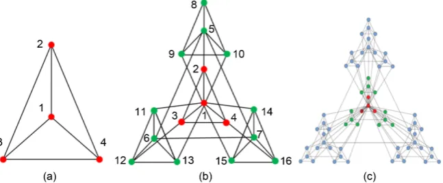
Taking the hierarchial network in Figure 1 as an example, its construction processes are as follow:

Figure 1(a) is the initial module, a complete graph made up of four nodes, and then we select node 1 as a center node while other nodes are called peri-pheral nodes;

Make three copies of Figure 1(a), link all peripheral nodes (node 8 - 16) of three copies with the central node (node 1) of the initial network together, and then connect the central nodes (node 5 - 7) from three copies which form the two layers network as shown in Figure 1(b).

Next, Make three copies of Figure 1(b), then link all the most peripheral nodes (the nodes corresponding to node 8 - 16 in the replica) with the central node of initial network (node 1) together. Finally, connect the central node (the node corresponding to node 1 in the replica) of three copies together, forming a three layers network model as shown in Figure 1(c). And so on, a hierarchical network model with more layers can be constructed.

There are I

M nodes in the network with I layer (in which, M is initial network node number). We can see from the network structure and Figure 1(c) that the hierarchical network is extremely regular, and has obvious characteris-tics of hierarchy and module, and even self-similar feature. We will study the synchronizability and the optimization problem of hierarchical network.

2.2. Description of Network Synchronizability

Considering a dynamic network with numerous identically dynamical systems as nodes, its state equation is:

( )

(

( )

)

(

( )

)

1

, 1, 2, ,

N

i i ij j

j

x t x t δ x t i N

=

=F −

∑

L H =

  (1)

Among which, m i

[image:3.595.213.537.559.693.2]

x∈R is the state variables of i node, x t_i

( )

=F

(

x t_i

( )

)

is the dynamic equation of i node. The constant δ >0 is the coupling strength

DOI: 10.4236/cn.2017.93015 210 Communications and Network and H

( )

. :Rm→Rm is the internal coupling function between the state va-riables of each node.

( )

N N

ij _{N N}

× ×

= ∈

L L R is the Laplace matrix of the network (external coupling matrix).

When t→ ∞, it satisfies

( )

( )

lim i

t→∞x t =S t (2)

Then the dynamic network (1) is said to achieve synchronization. The syn-chronization manifold is the solution to the isolated node equation, satisfying

( )

(

( )

)

s t =F s t (3) Mark that the synchronization area of the network (1) is C, and the eigenva-lue of the matrix

( )

N N

ij _{N N}

× ×

= ∈

L L R is λk,k=1,,N. From the main stabil-ity function theory, when λk satisfied

, 2, ,

k C k N

δλ ∈ = _

The synchronization manifold of network (1) is asymptotically stable. Ac-cording to the different situations of the synchronous region, we generally divide the network into three types shown as follow.

Type I network: the synchronous region is C= −∞

(

,

α α

1

)

, 1<0

Type II network: the synchronous region is C=

(

α α α

1, 2

)

, 2<

α

1<0

Type III network: the synchronous region is an empty set. This type of net-work cannot achieve the synchronous state for any coupling strength and coupling matrix.

In addition, there are also synchronous regions for multiple limited regions, but such network is rare.

This type of network is determined by the internal and isolated node dynam-ics of the network, which is irrelevant to the topology of the network. For net-works of type I and type II, only when it satisfied δλ2>α1 or λ λN 2<α α2 1,

the synchronous flow of the network can be asymptotically stable (λ2, λ λN 2

is the minimum non-zero eigenvalue of corresponding Laplace matrix and the maximum nonzero eigenvalues), and when λ2 gets bigger or λ λN 2 gets

smaller, the network synchronous ability will be stronger. Therefore, we usually use λ2 or λ λN 2 to depict network synchronizability.

3. The Analysis of Hierarchical Network Synchronizability

This section makes a numerical simulation with different initial module node number and different layers of the hierarchical network model respectively. Through the comparison of the changes of λ2 and λ λN 2, we analyze the

in-fluence of the size of the initial module and network layer on hierarchical net-work model synchronizability.

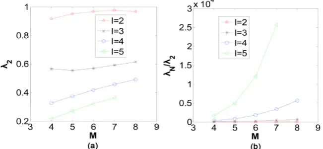
3.1. The Impact of Initial Module Size on Synchronizability

net-DOI: 10.4236/cn.2017.93015 211 Communications and Network work of initial nodes M=4, M =5, M=6, M =7, M =8 respectively.

In Figure 2(a), Figure 2(b), the relationships between λ2、λ λN 2 and the

number of initial network nodes are given. And it can be seen from the figure that with the increase of the number of initial network nodes, at that time,

4

I ≥ the whole λ2 presents an increasing state, but λ λN 2 monotonically

increasing.

This shows that for the type I network, when the layer number of the hierar-chical network is certain, the synchronizability of the hierarhierar-chical network in-creases with the increase of the number of initial module nodes. On the other hand, for type II hierarchical network, its synchronizability decreases with the increase of the number of initial module nodes.

3.2. The Impact of Network Layer Number on Synchronizability

When the number of layers is certain, the study on the relationship between the initial module size and the network synchronizability can only provide a hori-zontal comparison between the different networks. By contrast, based on the mechanism of the hierarchical network, the influence of hierarchical network layer on the network synchronizability has more research values which can pro-vide magnificent guidance of analysis and design for the generation and growth of the hierarchical network.

It can be seen by observing the Figure 3(a), Figure 3(b) that with the increase of the number of layer network, it decreases slowly and increases exponentially. This shows that, regardless of type I or type II hierarchical network, with the growth of network layer number, network synchronizability reduces. In particu-lar, for type II hierarchical networks, the network's synchronizability declines dramatically as the number of layers grows.

4. The Optimization of Layer Network Synchronizability

4.1. Improvement of the Synchronizability of the Network by

Reducing the Maximum Network Node Betweenness

[image:5.595.213.539.552.702.2]

Because the general network synchronizability is negatively related to the

[image:6.595.273.472.433.647.2]

DOI: 10.4236/cn.2017.93015 212 Communications and Network Figure 3. The relation between layer number I and λ₂, λ λ_{N 2}.

maximum betweenness, which means the largest node betweenness is, the worst the network synchronizability is. We try to improve the synchronizability of the network by reducing the maximum node betweenness.

Large-scale hierarchical network belongs to the network of node betweenness with great differences. In order to effectively reduce the network center node betweenness, we apply the method of Segmentation to make a tiny perturbation in the Internet structure to reduce the maximum network node betweenness and improve the synchronizability of the network.

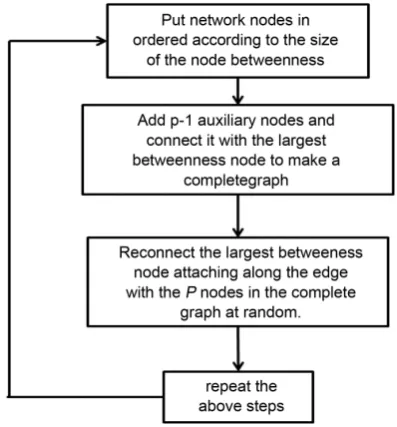
The structural perturbation procedure of “Segmentation method” is as fol-lows:

In order to study the effect of “segmentation method”, we compare the changes of the maximum node betweenness bmax, λ2, λ λN 2 before and after

numer-DOI: 10.4236/cn.2017.93015 213 Communications and Network ical Simulation.

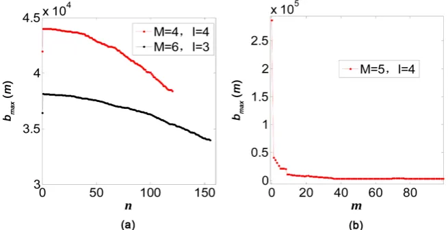
Figure 4(a) is changes of maximum node betweenness bmax in the process of

segmenting the maximum node betweenness of two models in initial node 4

M= , layer I=3 and the initial node M =6, layer I=3. The leap of b_max between the number of 0 and 1 in the reconnective operation times is caused by adding auxiliary nodes. In the process of reconnective operation after the single partition, the maximum node betweenness of the network decreases sharply. In the process of reconnective operation after the single partition, the maximum node betweenness of the network decreases sharply. bmax decreases from

4

4.20 10× and 3.80 10× 4 to 3.64 10× 4 and 3.40 10× 4. Figure 4(b) is changes of maximum node betweenness bmax in the process of “5-segmention” in the

hierarchical network when initial node number M =5,I=4. After operating “5-segmention” for 100 times, bmax decreases from

5

2.87 10× to 4 1.07 10× . Therefore, the segmentation method has a great impact on reducing the maxi-mum node betweenness of the hierarchy network.

Taking the hierarchial network as an example when M =5,I=4, the net-work has 625 nodes and the maximum betweenness of four nodes is 5

2.87 10× , 4

4.32 10× , 5.53 10× 3, 5.48 10× 3, and the number of corresponding nodes is 1, 4, 4 and 16 respectively. Due to segmenting for several times, there are multiple nodes that have the maximum node betweenness of network (For example, after segmenting for several time, the maximum node betweenness of network

be-comes 4

4.32 10× . At this point, four nodes in the network will have the maxi-mum node betweenness of network.) Therefore, in the process of repeating “segmentation”, no every operation can reduce the maximum node betweenness of network.

[image:7.595.210.538.492.660.2]

As shown in Figure 5(a), with the increase of the times of “segmentation”, the whole λ2 is in the periodical growth status. When the “segmentation” operation

Figure 4. The changes of the maximum betweenness during the “segmentation” process. (a) In the process of single “segmentation” reconnection, the maximum network node betweenness bmax changes with number of reconnection edge n; (b) The maximum

[image:8.595.210.537.67.231.2]

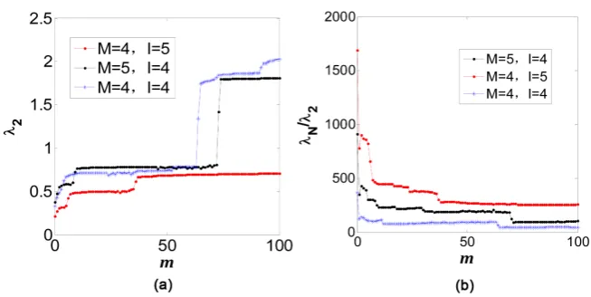
DOI: 10.4236/cn.2017.93015 214 Communications and Network Figure 5. λ2, λ λN 2 change with the “segmentation” times of m.

can reduce the maximum node betweenness of network, λ2 can grow

substan-tially. When the “segmentation” operation can not reduce the maximum node betweenness of network, λ2 enters the periodically tiny perturbations.

It can be seen from Figure 5(b) that λ λN 2 greatly reduces after the first

“segmentation” operation, but after the second “segmentation”, there is a rela-tively slight increase, and it enters into the periodically reduced state in the sub-sequent “segmentation” operation. When the "segmentation" operation can re-duce the maximum node betweenness of network, λ λN 2 can reduce

substan-tially; when the “segmentation” operation can not reduce the maximum node betweenness of network, λ λN 2 enters the periodical tiny perturbations.

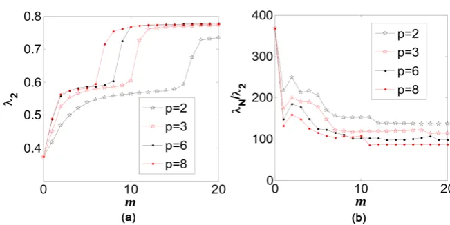
Figure 6 is the numerical simulation result between “segmentation” opera-tions times and λ2, λ λN 2 when two hierarchical networks M =5,I=4, and

4, 4

M = I= at different p values, This result is the average of the operative results after 10 times.

We observed that different p have a greater effect on the changes of λ₂ and λ λN 2 in Figure 6. In general, after selecting the appropriate p value,

2

λ _{will increase to two times as its original one after the second jump.}

The change of λ λN 2 is more special, although the change is less stable,

since λ λN 2 will drop to about 1/2 after the first segmentation. At this time, we

believe that the network synchronizability has been improved to a certain extent. In order to maintain the other characteristics of the network, the “segmentation” should be terminated.

To sum up, the Segmentation Method can effectively reduce the network’s maximum betweenness of nodes, and the synchronizability of the hierarchical network is significantly improved.

4.2. Improving Network Synchronization by Reducing the

Average Path

In this section, we try to reduce the average path length of the network and im-prove the synchronizability of the network.

DOI: 10.4236/cn.2017.93015 215 Communications and Network Figure 6. The influence of p on the change of λ2, λ λN 2 in “p-segmentation”. (a)

Network model is M =5,I=4; (b) Network model is M =4,I=4.

Method, which can change the rest of the network structure characteristics without changing the degree of each node in the network conditions and sepa-rately discuss two controversial structure characteristics of network average and the degree distribution. However, due to the complete randomness of the ran-dom crossing method, no every cross-connection can achieve the goal of reduc-ing the average distance of the network. In the experiment, it was found that a large number of random cross-linking was invalid.

In the experiment based on the hierarchical network model, the operational efficiency of random crossing method is very low, and the effective rate is often less than 1%. In order to ensure the reconnective operation can effectively re-duce the average distance of the network and preserve the characteristics of con-stant node degree at the same time. We put forward a new reconnection me-chanism-Parallel reconnection method, shorthand for PRC method (Parallel re-connection).

In order to investigate the influence of the mean distance of the hierarchical network on its synchronizability, we use the PRC method to change the average distance of the network.

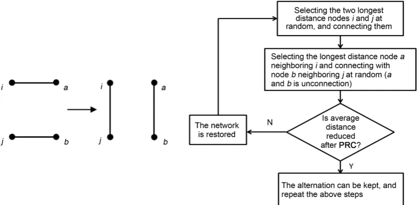
We make every reconnective operation with a purpose. The steps of the PRC method are as follows:

1) Selecting the two longest distance nodes i and j in the network at random, and connecting them.

2) Selecting the longest distance node a neighboring i and connecting with node b neighboring j at random (a and b is unconnection).

3) Judging whether the average distance is reduced after reconnecting the network. If it does, it works and the alternation can be kept. Otherwise, the net-work will be restored to the previous unreconnected state.

4) Repeating steps (1)-(3) until achieve the average distance or pre-set opera-tion times of the desired network.

[image:9.595.208.534.65.228.2]

DOI: 10.4236/cn.2017.93015 216 Communications and Network Therefore, when L>3, we do not need to judge whether the selected nodes are connected with other nodes in the PRC method, they can directly parallel reconnect. At this time, the operational efficiency of the PRC Method is very high, which can not only improve the effect of reducing the average distance of the network, but also keep the nodes and degrees of the network unchanged at the same time (Figure 7).

[image:10.595.119.535.296.500.2]

On the other hand, for different hierarchical network models, PRC method, a limitation is that after a certain number of effective reconnections, the effective-ness of the reconnection will fall sharply, so that PRC method reduces the hie-rarchical network average distance limitation. But before that, almost every pa-rallel reconnection can reduce the network average distance, and the efficiency of the PRC operation can be maintained over 90%.

[image:10.595.302.446.551.679.2]

Figure 8 is the simulation results of average distance of three hierarchical networks and the times for effectively PRC when M =5,I=4, M =6,I=4

Figure 7. Schematic diagram of PRC, among them, i and j are the longest two nodes in the network, a and b are the two longest nodes in the neighbor nodes of i and j.

DOI: 10.4236/cn.2017.93015 217 Communications and Network and M =7,I=4. The result is 10 times the average operational results. The ef-ficiency of PRC operation is about 93%, 94% and 97%. It can be seen from the Figure 8, Figure 9(a) and Figure 9(b). Taking the hierarchical network model of M =5,I=4 as an example, after 100 times of effectively PRC, L decreases constantly, and gradually decreases from 3.1695 to 3.0173. At the same time, λ2

increases from 0.3736 to 0.6842 and λ λN 2 decreases from 912.7612 to

474.9729.

This shows that the smaller the average distance of the network is, the easier the network is to achieve synchronization, and the stronger capability of net-work synchronizability. However, a large number of simulative experiments have found that although hierarchical network synchronizability can get stable improvement in the situation of keeping the network degree and degree distri-bution unchanged. But for some hierarchical networks, the changes of λ2 and

2 N

λ λ _{sometimes are small, and the PRC method seems to be limited in} en-hancing the network synchronizability.

5. Conclusions

This paper mainly studied that a hierarchical network of self-similar module structure synchronizability is associated with the initial module size and the layer number of network. The study found out that when the network layer was and remained unchanged, for type one network, the initial module of hierar-chical network node number would increase, and the network synchronizability would be stronger. On the other hand, for type two hierarchical networks, the synchronizability weakened with the increase of the number of initial module node. While for the hierarchical internet of the same initial number of nodes, with the increase of network layers, the network would become increasingly dif-ficult to achieve synchronization.

[image:11.595.212.537.551.706.2]

As for the problem of hierarchical network synchronizability and optimiza-tion, “Segmentation Method” can reduce the maximum node betweenness. When the value of p can be chosen appropriately, network synchronizability can be greatly improved. The PRC method proposed in this paper is to optimize

DOI: 10.4236/cn.2017.93015 218 Communications and Network network synchronizability by reducing the average distance of the hierarchical network. Though the method is deficient in improving the extent of hierarchical network synchronizability, its stability is good. And the PRC method can subtly and separately analyze the two controversial structure characteristics—average distance and degree distribution, which changes its hierarchical network average distance only and the degree distribution remains unchanged.

Although these two methods can both improve the synchronizability of hie-rarchical network, but which one is better? Whether these two methods are also applicable to other types of web? There are more questions for us to delve into and that is our direction to head for in the future.

Acknowledgements

This work is supported by the National Natural Science Foundation of China under Grant 61563013 and 61663006.

References

[1] Wang, X.F., Li, X. and Chen, G.R. (2004) The Theories and Applications of Com-plex Networks. Tsinghua University Press, Beijing.

[2] Li, Z.J., Wang, T., Yang, Y.G., et al. (2007) Structural Analysis Based on the Hierar-chical Modularity and Power-Law Feature Points of Internet Topology. Science Technology and Engineering, 7, 5791-5794.

[3] Zhao, M. (2007) Research Progress of Dynamic System Synchronization on Com-plex Network. University of Science and Technology of China, Hefei.

[4] Wang, X.F. and Chen, G.R. (2002) Synchronization in Small-World Dynamical Networks. Bifurcation and Chaos, 12, 187-192.

https://doi.org/10.1142/S0218127402004292

[5] Wang, X.F. and Chen, G.R. (2002) Synchronization in Scale-Free Dynamical Net-works: Robustness and Fragility. IEEE Transactions on Circuits and Systems I, 49, 54-62.https://doi.org/10.1109/81.974874

[6] Barahona, M. and Pecora, L.M. (2002) Synchronization in Small-World Systems. Physical Review Letters, 89, 054101.https://doi.org/10.1103/PhysRevLett.89.054101 [7] McGraw, P.N. and Menzinger, M. (2005) Clustering and the Synchronization of

Oscillator Networks. Physical Review E, 72, 015101.

https://doi.org/10.1103/PhysRevE.72.015101

[8] Nishikawa, T., Motter, A.E., Lai, Y.C., et al. (2003) Heterogeneity in Oscillator Networks: Are Smaller Worlds Easier to Synchronize? Physical Review Letters, 91, 014010.https://doi.org/10.1103/PhysRevLett.91.014101

[9] Hong, H., Kim, B.J., Choi, M.Y. and Park, H. (2004) Factors That Predict Better Synchronizability on Complex Networks. Physical Review E, 69, 067105.

https://doi.org/10.1103/PhysRevE.69.067105

[10] Chen, J.Y. and Lu, J.G. (2013) Synchronous Control of Dynamic Complex Network with Switching Topology. Science Technology and Engineering, 13, 2720-2725. [11] Dai, X.L. (2008) The Study on the Synchronous Behavior of Dynamic Systems on

Complex Networks. Nanjing University of Aeronautics and Astronautics, Nanjing. [12] Zhang, H., Wei, D., Hu, Y., et al. (2014) Modeling the Self-Similarity in Complex

Submit or recommend next manuscript to SCIRP and we will provide best service for you:

Accepting pre-submission inquiries through Email, Facebook, LinkedIn, Twitter, etc. A wide selection of journals (inclusive of 9 subjects, more than 200 journals)

Providing 24-hour high-quality service User-friendly online submission system Fair and swift peer-review system

Efficient typesetting and proofreading procedure

Display of the result of downloads and visits, as well as the number of cited articles Maximum dissemination of your research work

Submit your manuscript at: http://papersubmission.scirp.org/