Numerical Experimental Updating Identification of Elastic Behavior of a Composite Plate Using New Multi Objective Optimization Procedure

Numerical-Experimental Updating Identification of Elastic

Behavior of a Composite Plate Using New Multi-Objective

Optimization Procedure

Samir Ghanmi1*_{, Sofiane Bouajila}2_{, Mohamed Guedri}3

1_{Nabeul Preparatory Engineering Institute-IPEIN, Nabeul, Tunisia;} 2_{Higher Institute of Technological Studies of Nabeul, Nabeul,}

Tunisia; 3_{Higher School of Science and Technology of Tunis, Tunis, Tunisia.}

Email: *_{[email protected]}

Received August 6th_{, 2012; revised September 2}nd_{, 2012; accepted September 8}th_{, 2012}

ABSTRACT

This work focuses on the updating-based identification of the three-dimensional orthotropic elastic behavior of a thin carbon fiber reinforced plastic multilayer composite plate. This consists in identifying the engineering constants that minimize the relative deviations between the first eight experimental and three-dimensional finite element frequencies of the vibrating free plate. For this purpose, a multi-objective optimization procedure is applied; it exploits a Particle Swarm Optimizer algorithm (PSO) that is coupled to a metamodeling by the new response surfaces method procedure (NRSMP); the latter is based on numerical design experiments. The conducted sensitivity analyses indicate that the four engineering constants of the two-dimensional elasticity are the most influent.

Keywords: Composites; Finite Element Experimental Designs; Multi-Objective Optimization; Numerical-Experimental Updating Identification; Response Surfaces

1. Introduction

During the last three decades, composite materials are widely used in modern structures for high performance and reliability because of their high strength, specific stiffness, light weight and adjustable properties. However, before using this type of material with confidence in in- dustrial applications such as marine, automotive or aero- space structural components, a thorough characterization of the constituent material properties is needed. Because of the number and the inherent variability of the constitu- tive properties of composite materials, the experimental characterization is quite cumbersome and requires a large number of specimens to be tested.

To circumvent this lack, an effective procedure consists in using mixed numerical-experimental methods which constitute powerful tools for estimating unknown consti- tutive coefficients in a numerical model of a composite structure from static and/or dynamic experimental data collected on the real structure.

Starting from the measurement of quantities such as the natural frequencies and mode shapes, these methods allow, by comparing numerical and experimental observations, the progressive refinement of the estimated material properties in the corresponding numerical model. In this

domain, dynamic mixed techniques have gained in im- portance owing to their simplicity and efficiency [1,2].

In this work, a new mixed numerical-experimental identification method based on the use of a multi-objec- tive optimization procedure. It exploits a Particle Swarm Optimizer algorithm (PSO) [3-5] that is coupled to a meta-modeling by the new response surfaces method procedure (NRSMP) based on Droesbeke et al. and Myers

et al. works [6,7]; this procedure is applied to estimate unknown constitutive parameters from a numerical model of a composite plate and its experimental data of dynamic tests.

This method is based on a technique for minimizing the differences between the first eight numerical frequencies of the composite structure and the corresponding ex- perimental modal values [8].

In our case, the constitutive parameters that can be identified are three in-plane Young’s moduli E1, E2 and E3

and the in-plane and transverse shear moduli G12, G13 and

G23, the Poisson’s ratios v12, v13 and v23.

This optimization procedure is preceded by a sensitivity analysis using ANOVA [7] in order to eliminate non- influent parameters on the behavior of the composite structure.

The multi-objective problem to be solved is of eight cost functions and nine design parameters which are: E1,

E2, E3, G12, G13, G23, v12, v13 and v23.

2. Elastic Behavior of Composites

The macroscopic mechanical properties of composite materials depend on their microstructure. The micro structural organization that is generally not regular, often leads to anisotropy at the macroscopic level. This anisot- ropy can be explained mechanically as a dependency of the elastic response vis-à-vis the direction of stress.

However, for most of the industrial composites, this behavior is often orthotropic, described by the stress- strain relationship:

i Cij j

   (2.1) where the terms i and j represent components of the

stress and strain tensors, respectively. ij is the matrix of

elastic coefficients. The matrix of elastic coefficients for an orthotropic material is written as follows:

C

11 12 13

22 23 33 44 55 66 ij

C C C C C C C C Sym C C                     (2.2)

There are twelve non-zero components of which nine are independent. (2.1) can be rewritten in terms of the compliance matrix, S_ij:

j Sij i

   (2.3)

The compliance matrix for an orthotropic material ex- pressed in terms of elastic properties such as Young’s modulus, shear modulus and Poisson’s ratio and is:

31 21

1 1 1

32 12

1 2 2

13 23

1 2 3

1 23 13 12 1 1 1 1 1 1 ij ij

E E E

E E E

E E E

C S G G G                                                   

  (2.4)

where Ei are the Young’s moduli in the i direction, vij are

Poisson’s ratio for strain in the j direction with stress applied in the i direction, and Gij are the shear moduli in

the i-j plane (i, j = 1, 2 or 3). Since the matrix of elastic coefficients and the compliance matrix are symmetric, hence

ij ji

i j

E E

 

 (2.5)

3. Problem Data

We studied a composite plate that was cut by the manu- facturer from a large panel of length 1.56 m, width 1.06 m, 4.16 mm in thickness and density of 1512 kg/m3_{. The}

panel material is of IMS/977-2 type (Figure 1). The panel consists of 16 layers with the stacking sym- metric sequence of [90/45/0/-45]2S: its elastic properties

are provided by the manufacturer (modulus in GPa):





1 2 12 12

3 2 13 12 13 12

23 12 23

160; 8.6; 4.85; 0.32

; ;

2

3.2; 0.4 estimate 3

E E G

E E G G

G G               (3.1)

The plate was provided by the manufacturer with the following nominal dimensions : 300 mm in length (y axis) and 200 mm wide (x axis); however, the checks in the laboratory, provides [8]a width of 200.3 mm, an average thickness of 4.2 mm and a density of 1521 kg/m3_{. It is}

these data that were used to make a first simulation of the free plate configuration using 3D solid elements Quad- ratic hexahedral ABAQUS® _{element C3D20R: to 17303}

nodes, 2400 elements: 51909 dof.

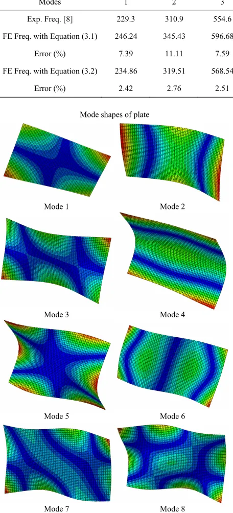
Figure 2 shows the first eight modes of the plate to be studied.

The measured frequencies [8]and simulated, are pro- vided in Table 1 for the first eight modes of vibration free. We note that numerical frequencies greatly overestimate

X Y

Z

(a) (b)

Figure 1. Tested plate (a) and 3D FE model (b). (a) Tested omposite plate [8]; (b) 3D FE model.

c

Table 1. Experimental frequencies (Hz) and simulated by FE of the composite plate.

Modes 1 2 3 4 5 6 7 8

Exp. Freq. [8] 229.3 310.9 554.6 581 724.7 889.1 1068.4 1163.7

FE Freq. with Equation (3.1) 246.24 345.43 596.68 608.49 775.66 972.84 1142.7 1264.6

Error (%) 7.39 11.11 7.59 4.73 7.03 9.42 6.95 8.67

FE Freq. with Equation (3.2) 234.86 319.51 568.54 594.66 740.27 912.01 1095.3 1194.3

Error (%) 2.42 2.76 2.51 2.35 2.14 2.57 2.51 2.62

Mode shapes of plate

Mode 1 Mode 2

Mode 3 Mode 4

Mode 5 Mode 6

Mode 7 Mode 8

Figure 2. First eight modes of the composite plate.

those measured, suggesting that elastic properties of the plate, given by manufacturer, overestimate those of the plate tested. Measurements on another plate of the same nominal size, also cut by the manufacturer from the same large panel, provided an average thickness of 4.13 mm and a density of 1547 kg/m3_{, these new data confirm that}

the material of panel is not uniform and identification of

its elastic properties is required; this plate gave the fol- lowing constants (modulus in GPa) [9]:

1 2 12 12

13 23 3 2 13 12 23

129.8; 10.9; 5.7; 0.37;

4.4; 3.2; ; ; 0.55

E E G

G G E E



  

   

     (3.2)

These results confirm that the design parameters pro- vided by the manufacturer are generally largely overes- timated or underestimated.

The obtained frequencies are shown in Table 1. We denote this time that correlation between experiment and calculation is satisfactory; the residual errors indicate that they are probably due to differences in the dimensions (width and thickness) and densities of the two plates.

It is therefore proposed, in what follows, to identify elastic constants of this plate by updating the experimental frequencies [8] and simulated by ABAQUS® _{3D FE using}

a proposed multi-objective optimization procedure re- taining the data (Equation (7)) as initial values and we take as variations on the parameters ±20% around their mean values.

4. Identification by Multi-Objective

Optimization Procedure

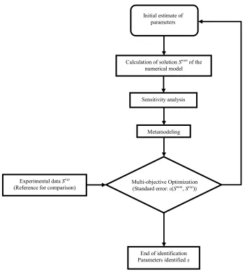
Figure 3 presents the proposed methodology for the identification of mechanical properties of the composite plate (Figure 1).

Its three main steps are detailed in the following.

4.1. Sensitivity Analyze

Sensitivity analysis studies the “sensitivity” of the outputs of a system to changes in the parameters, inputs or initial conditions which are often poorly known. Its goal is to show the effects of changing parameter values and their interactive effects and then eliminate those that are not significant on the output.

Initial estimate of parameters

Calculation of solution Snum _{of the}

numerical model

Sensitivity analysis

Metamodeling

Multi-objective Optimization (Standard error: ε(Snum_{, S}exp₎₎

Experimental data Sexp

(Reference for comparison)

End of identification Parameters identified x

Figure 3. Proposed procedure of identification.

turn any standard design into a robust one.

4.2. Metmodeling by New Response Surface Method Procedure

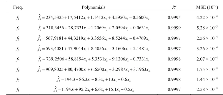
The metamodeling is based on the use of NRSMP which is based on the use of numerical design of experiments. The aim is to represent each frequency by a polynomial which will be easier to use in the optimization phase.

The linear models used here are second-order regres- sion models (4.1). A RSM for k input variables can be stated as:

1 1

2 0

1, 2

ˆ _{i i ij i j ii i}

i k

i j

i

k k

i

j

y   x  x x  x



  



 







(4.1) This model requires at least 2n + 1 + n(n− 1)/2 simu- lations to be completely defined. Where y is the response variable, x are the input variables, and the β’s are the

coefficients to be estimated.

Equation (4.1) may be written in matrix notation as: Y X  (4.2) where

1 2

n

y y Y

y       

     

 ;

11 12 1 21 22 2

1 2 1

1

1

k k

n n nk

x x x

x x x

X

x x x

 

 

 

 

 

 



 

   



1 2

n

;

 

        

     



1 2

n and

 

        

     



Use of only one configuration (a metamodel) which considers the real response appears in sufficient owing to the fact that it can be statistically far from the most precise polynomial which can be considered as the exact response. To surmount this disadvantage, we propose a method which aims to obtain the met model (polynomial) nearest to the reference. The components stages of the method suggested for obtaining the adequate met model are summarized as follows:

1) Number of design parameters (n); 2) Complete factorial design;

3) Random generation of “k”polynomials;

4) Statistical and frequency criteria satisfied or go to step 2;

5) Calculation of the polynomial average Pm: where

nrest is the number of the noted remaining polynomials

Prest:

1 rest n rest i m rest P P n 





Note: The designer generates randomly several poly- nomials of the function to estimate. Each polynomial obtained is evaluated statistically (MSE criterion for example). The set of polynomials that did not meet the criteria for evaluation constitute: Prest.

6) Generation of several samples of size “p” by Latin hypercube method (LHC);

7) Acceptable error of prediction εmor go to step 2.

The statistical criteria of selection are:  The error MSE which is defined by :





1 2 ˆ m i i i exact y y MSE

m   





where exact is the standard deviation of exact response

yi.

In practice, to satisfy of a process of the 6 sigma crite- rion an error MSE should not exceed value 0.09028 [10].  The coefficient of determination R2 _{is defined by:}









1 m_{i i i}

m i i i y y R y y      





where i is the exact response; is the estimated

response and

y yˆ_i

i

y is the mean value of the exact response. This coefficient must be as close as possible to value 1 (0

< R2_{<1) [6,7].}

4.3. Multi-Objective Particle Swarm Optimization

In mechanical engineering, the optimization problems are often multi-objective. The cost functions are complex (multimodal, non-convex, etc.) and there are generally

conflicts between them. Therefore, it is necessary to choose a multi-objective optimization strategy which can lead to the best alternatives among several.

Generally, a multi-objective optimization problem is expressed by:

 



   

 



minF x f x f x, , , f xn T

x S  _      (4.6)

where f x f x1

   

 

T

are cost functions,





x x x  x

n

S R is the vector of n optimization pa- rameters, represent the set of realizable solutions and F x

 

In this study, we exploit the multi-objective Particle Swarm Optimization algorithm (PSO). This is justified by several reasons. In fact, Particle swarm optimization (PSO) is a stochastic optimization method often used to solve complex engineering where the solution may be repre- sented as a hyper dimensional vector (such as 3D space). The method’s strength lies in its simplicity, being easy to code and requiring few algorithm parameters to define convergence behavior.

Similar to evolutionary optimization methods, PSO is a derivative-free, population-based global search algorithm. PSO uses a population of solutions, called particles, which fly through the search space with directed velocity vectors to find better solutions. These velocity vectors have sto- chastic components and are dynamically adjusted based on historical and inter-particle information [11,12].

5. Identification of Elastic Behavior of the

Composite Plate

The proposed identification procedure, which based of multi-objective optimization, is applied here to this com- posite plate described above. Multi-objective problem to be solved is in eight cost functions (5.1).

 

 

 





exp exp

1 2 3 12 23 12 13 23 ˆ

min ; 1, ,8

, , , , , , ,

i i

i

i

f x f

F x x i

f

x E E E G G

     _       _   (5.1)

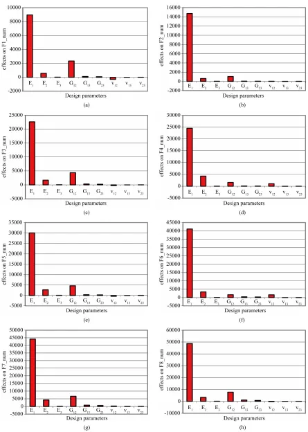
5.1. Sensitivity Analysis

A 2k _{factorial design of experiments was used. The use of}

nine design parameters (factors), each at two levels lead- ing to a total of 29 _{= 512 numerical experiments to be}

performed. These parameters vary in fields of ±20% around their mean values given by (3.2). To make this analysis, an ANOVA was performed for a significance level of 5%, that is to say, for a confidence level of 95%. There is a significant variation of E1, which is the most

and a slight variation on each of the parameters E2, E3, G12,

G23, v12, v13 and v23(Figure 4). The transverse parameters

E3, G13, G23, v13 and v23 have no significant effect. Three

in-plane parameters, E1, E2, G12, are most influential,

especially E1. From this analysis we find that the E1, E2,

G12, v12 factors.

This problem replaces the multi-objective problem of Equation (5.1).

The application of multi-objective optimization pro- cedure, with coupling PSO algorithm with metamodels (cost functions) of Table 2, led to the optimal values of design parameters that are given (after rounding) in Ta- bles 3 and 4.

5.2. Metamodeling by Response Surface Method Table 3 shows the values of design parameters pro- vided by the manufacturer and those given by optimiza- tion. These values are compared each time by the mean values of design parameters. The variations of parame- ters (Table 3) show that the manufacturer has underesti- mated the parameters E2, E3, G12, v12, v13 and v23 and

overestimated parameters E2 and G23.

In this phase, we consider the results of sensitivity analy- sis above. The new problem is thus to four design pa- rameters (significant parameters), each at two levels leading to a total of 24 _{= 16 numerical experiments to be}

performed. These parameters vary in fields of ±20%

around their mean values given by (3.2). _{Table 4 presents the eight frequencies from this opti-} mization and residual errors (both rounded). Note that these errors are very satisfactory.

The non significant factors are frozen in their mean values.

The metamodels for each of the frequencies of the first eight vibration modes of free composite plate are given

by the equations in Table 2.

6. Conclusions

Each polynomial is statistically validated by a factor of determination R², which should be as close as possible to 1, and an MSE (Mean Square Error), which must be less than 0.09028 [10].

The updating-based identification of the three-dimen- sional orthotropic elastic behavior of a thin carbon fiber reinforced plastic multilayer composite plate is pre- sented.

Note that the metamodels (polynomials) of Table 2

meet all these criteria. This allows us to use these poly- nomials in the optimization phase.

This consists in identifying the engineering constants that minimize the relative deviations between the first eight experimental and three-dimensional finite element frequencies of the vibrating free plate.

5.3. Multi-Objective Optimization Procedure _{For this purpose, a new multi-objective optimization}

procedure is applied; it exploits a Particle Swarm Opti- mization algorithm that is coupled to a meta-modeling by new response surfaces method procedure; the latter is based on numerical design experiments. The conducted sensitivity analyses indicate that the four engineering constants of two-dimensional elasticity are the most in- fluent.

The multi-objective optimization is achieved by coupling the PSO algorithm to the metamodel. Taking into ac- count of the results of sensitivity analysis, the new multi- objective problem to be solved is:

 

 

 





exp exp

1 2 12 12 ˆ min

; 1, ,8

, , ,

i i

i

i

f x f

F x x

f i

x E E G





 _

 

 _



 _



 (5.2)

The proposed identification procedure confirms that the design parameters provided by manufacturer are gen-

Table 2. Estimated frequencies.

Freq. Polynomials R2 _{MSE (10}−7₎

f1 fˆ1234,5325 17,5412 x11.1412x24.5950x30.5600x4 0.9995 4.22 × 10

−4

f2 fˆ2318,3456 28,7331 x11.2069x22.0594x30.0631x4

4

0.9999 5.28 × 10−5

f3 fˆ3567,9181 44,3219 x13.3556x28.5244x30.4769x

4

0.9997 2.56 × 10−4

f4 fˆ4593,4081 47,9044 x18.4056x23.1606x32.1481x

4

0.9997 3.26 × 10−4

f5 fˆ5739,2506 58,8194 x15.3531x29.1206x30.7331x

4

0.9998 2.07 × 10−4

f6 fˆ6909,8025 80,4700 x16.6500x23.2987x33.1963x

4

0.9998 1.75 × 10−4

f7 fˆ7194.3 86.3 x18.3x213x30.6x

4

0.9998 1.44 × 10−4

f8 fˆ 1194.6 95.28  x16.6x215.1x30.5x 0.9997 2.58 × 10

(a) (b)

(c) (d)

(e) (f)

(g) (h)

Table 3. Optimal values and variations of design parameters.

Parameters E1 (GPa) E2 (GPa) E3 (GPa) G12 (GPa) G13 (GPa) G23 (GPa) ν12 ν13 ν23 Mean Values (M.M) (3.2) 129.8 10.9 10.9 5.7 4.4 3.2 0.37 0.37 0.55

Manufacturer (M) 160 8.6 8.6 4.85 4.85 3.2 0.32 0.32 0.40

Variation M/M.M (%) 23.27 −21.10 −21.10 −14.91 10.28 0 −13.51 −13.51 −6.27

After Optimization (A.O) 120.1 11.6 9.6 5.9 4.3 3.8 0.37 0.44 0.59

Variation A.O/M.M (%) −7.45 6.42 −11.93 3.50 −2.27 18.75 0 18.92 7.27

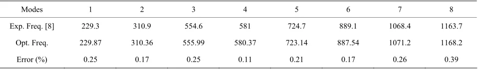
Table 4. Frequencies (Hz) after optimization and residual errors (%).

Modes 1 2 3 4 5 6 7 8

Exp. Freq. [8] 229.3 310.9 554.6 581 724.7 889.1 1068.4 1163.7

Opt. Freq. 229.87 310.36 555.99 580.37 723.14 887.54 1071.2 1168.2

Error (%) 0.25 0.17 0.25 0.11 0.21 0.17 0.26 0.39

erally largely overestimated or underestimated. Therefore, before using mechanical structures like composite plates, it makes sense to correctly identify their mechanical properties to avoid any further risks, hence the interest of our proposed identification procedure.

REFERENCES

[1] J. Cugnoni, “Identification and Registration Modal Fre- quency of Shell Constitutive Properties of Composite Ma- terials,” Ph.D. Thesis, Federal Polytechnic School of Lau- sanne, 2005.

[2] M. Hamdi, S. Ghanmi, A. Benjeddou and R. Nasri, “Identification by Multi-Objective Optimization of Three- Dimensional Elastic Behavior of a Multilayer Composi- te,” First International Symposium IMPACT, Djerba,2010. [3] M. Clerc and P. Siarry, “A New Metaheuristic for Diffi-

cult Optimization Method of Particle Swarm,” Vol. 3-7, 2004.

[4] J. Kennedy and R. C. Eberhart, “Particle Swarm Optimi- zation,” Proceedings of the IEEE International Confer- ence on Neural Networks, 1995, Vol. 4, pp. 1942-1948. doi:10.1109/ICNN.1995.488968

[5] J. F. Schutte, B. Koh, J. A. Reinbolt, R. T. Haftka, A. D. George and B. J. Fregly, “Evaluation of a Particle Swarm

Algorithm for Biomechanical Optimization,” Journal of Biomechanical Engineering, Vol. 127, No. 3, 2005, pp. 465-474.

[6] J. J. Droesbeke, J. Fine and G. Saporta, “Design of Ex- periments: Applications in the Company,” Paris, 1997. [7] R. H. Myers and D. C. Montgomery, “Response Surface

Methodology,” Wiley, New York, 2002.

[8] G. Chevalier and A. Benjeddou, “Coupling Effective Electromechanical Piezoelectric Composite Structures: Experimental and Numerical Characterization,” Journal of Composites and Advanced Materials, Vol. 19. No. 3, 2009, pp. 339-364.

[9] H. Friedmann, “Non-Destructive Parameter Estimation, in CASSEM D9-Test Report on Experimental Validation for Test/Model Correlation,” March 2008, pp. 5-13.

[10] G. J. Battaglia and J. M. Maynard, “Mean Square Error: A Useful Tool for Statistical Process Management,” AMP Journal of Technology, Vol. 34, 1996, pp. 1256-1260. [11] A. A. Groenwold and P. C. Fourie, “The Particle Swarm

Optimization in Size and Shape Optimization,” Structural and Multidisciplinary Optimization, Vol. 23, 2002, pp. 259- 267. doi:10.1007/s00158-002-0188-0