Munich Personal RePEc Archive
Interest Rate Rigidity and the Fisher
Equation
Belanger, Gilles
Ministere des Finances et de l’Economie de Quebec
25 February 2014
Online at
https://mpra.ub.uni-muenchen.de/57655/
Interest Rate Rigidity and the Fisher Equation
Gilles B´elanger
∗July 29, 2014
Abstract
I create a model where private banks face adjustment costs in nominal interest rates.
The model’s inflation responds to interest rate changes (both nominal and real) by
mov-ing in the opposite direction. That response justifies the Taylor rule and explains, through
credit conditions, the procyclicality of inflation. The model permits the analysis of
dif-ferent types of monetary policy using a variable inflation target. I use this feature to
simulate different policies and compare them to interest rate data from the last century.
The interest rate rigidity model leads to credit-conditions-driven inflation, which I
be-lieve is more realistic than competing models of inflation.
Keywords: Interest Rate Rigidity, Inflation, Monetary Policy, Fisher Effect.
JEL: E31, E43, E52.
∗Minist`ere des Finances du Qu´ebec; 12, rue Saint-Louis, Qu´ebec (Qu´ebec) Canada, G1R 5L3;
1
Introduction
On the onset of the crisis, the debate at the Fed about where inflation was going and more
recently at the Sveriges Riksbank highlight radical divergence of views. What we know about
inflation mostly consists of two stylized facts: its inverse relation with interest rates and
procyclicality. This paper offers an alternative model concentrating on these two stylized
facts, but also on credit conditions. Specifically, it examines whether rigidity in nominal
interest rates creates a simple and credible narrative for the behavior of inflation.
Interest rate rigidity has been discussed since Keynes, but the literature on interest rate
rigidity does not fully address its macroeconomic implications. Models rarely isolate the
effects of interest rate rigidity (or even credit frictions) from other factor affecting inflation,
keeping us from knowing what interest rate rigidity actually does to inflation. How nominal
interest rate rigidity interacts with the Fisher equation is simple, yet the implications are
interesting. If nominal rates cannot catch up to real rates, the Fisher effect becomes inverted
in the short term: central banks must lower interest rates to stimulate inflation, and credit
crunches lower inflation.
In the model, a private bank, facing adjustment costs, cannot fully adjust nominal rates
to account for changes in real rates. The other agent, a central bank, affects real rates while
monitoring their indirect effect on nominal rates (i.e. internalizing the reaction of the private
bank). The central bank does so to achieve its inflation target. How the central bank uses the
target provides a way to analyze monetary policy; for example, a variable target simulates a
peg to gold or to a foreign currency.
To visualize nominal interest rate rigidity, imagine a fictional case of constant nominal
interest rates: when the real interest rate goes up, inflation necessarily goes down. This is the
point made byCarmichael and Stebbing (1983), but it also happens when nominal interest
rate hit the zero lower bound.1
Research about interest rate setting points to sluggish pass-through from a central bank’s
key rate to market rates (interest rate pass-through), and from market rates to lending rates
(bank rate rigidity). Kobayashi(2008, Section 2) surveys the literature on interest rate
pass-through and de Bondt, Mojon and Valla (2005), on bank rate rigidity (see also Illes and
Lombardi(2013) for recent issues related to the financial crisis). Still, most of this research
focuses on empirical test for nominal interest rate rigidity, theoretical justifications for it,
or its microeconomic effects. Little research concentrates on the macroeconomic effects
of this rigidity. Exceptions includeRavenna and Walsh (2006) and Kobayashi(2008) who
investigate the implications of rate rigidity by incorporating them to standard models with
price rigidity (DSGEs).
Price rigidity is not a fact, but a way to explain its persistence, which is the actual
statisti-cal fact. In this paper, I ignore price rigidity. First, modeling both price and nominal interest
rate rigidities makes it hard to discern which has what effect. Second, for the sake of
parsi-mony, the model presented here does not need to be built on top of both the NKPC postulates
and the ones I propose. Third, as shown byCraig and Dinger(2014), nominal interest rates
display lower volatility in micro data than do prices. Fourth, if we take the view that both
prices and interest rates behave sluggishly, interest rate rigidity may dominate. Interest rates
stir profits more than prices or even wages because of the interest rates use in discounting
future profits, while only relative prices and real wages affect profits. I partially compensate
for this (as some might feel) oversight by comparing results with annual data; as shown by
Klenow and Malin(2010), most prices reset within a year. Annual data also permits me to
stretch the sample back to a time when, as shown byBenati(2008), persistence was absent.
As stated earlier, this paper focuses on rigidity coming from the market, not the central
bank. Macroeconomists may have ignored this type of interest rate rigidity because the
control of nominal rates by monetary authorities seems perfect as indicated by Figure 1.1
and 1.2 of Woodford (2003a). From that perspective, interest rate rigidity stems from the
central bank itself. For example, Woodford (2003b) considers the benefits for the central
bank of interest rate smoothing, while DSGE models commonly add the lag of interest rate
to the Taylor rule, as inChristiano, Eichenbaum and Evans (2005). But if nominal rigidity
stems from the market, the central bank can just push real rates by a lot to get the change it
wants in nominal rates. Perfect control does not imply direct control.
Section2 presents a model that yields rigidity through adjustment costs of nominal
in-terest rates of a private bank, given the real ones. The private bank wants to have the real
interest rate at its equilibrium value, but cannot immediately do so because of the cost of
adjusting the nominal rate. The equilibrium real interest rate appears when inflation reaches
the central bank’s target or when there is no monetary policy.
Section 3 presents numerical illustrations in the form of impulse response functions
(IRFs) and simulations. The IRFs show how inflation targeting reduces real interest rates
volatility. Anticipated shocks suggest that the preemptive nature of nominal adjustments
ex-plains the price puzzle fromSims(1992). Then, I simulate three different monetary policies
with the model using the central bank’s inflation target process: a volatile inflation target
sim-ulates the Gold Standard; a constant target simsim-ulates inflation targeting; and a variable, but
persistent target simulates the period characterized by gradually rising inflation in the
sev-enties and declining inflation in the eighties. The simulations show we can model different
episodes of inflation and interest rate movements of the last hundred years simply through
monetary policy shocks, that is to say without changing the nature of the other shocks.
Sim-ulations also suggest inflation targeting reduces real interest rates volatility, while a gold
2
The model
The model leads to three equations that determine inflation, real and nominal interest rates.
The rigidity equation translates real interest rates into nominal interest rates. The Fisher
equation translates real and nominal interest rates into inflation. Finally, the real interest rates
equation comes from the real economy, but with feedback from monetary policy. A larger,
more complete, model would be superfluous: there is no point in defending the postulates
necessary to build it and it would make this paper overly long and complicated.
Agents in the model consist of a private bank, a central bank and an exogenous real
econ-omy. The private bank sets nominal interest rates. The real economy sets a real interest rate
(according to intertemporal preferences, the marginal productivity of capital, from abroad or
whatever source). Finally, the central bank affects real interest rates (through open market
operations and the like) in order to achieve an inflation target. Inflation influences the real
economy only because of the central bank’s actions.
The private bank acts as the stylized representation of the financial market. It minimizes
the gap between the real interest rate and what the rate would be under a binding inflation
target, but faces quadratic adjustment costs of changing nominal interest rates,
min
it
(
Et
" ∞
∑
s=0
βs rt+1+s−rt∗+1+s
2
+θ(it+s−it−1+s)
2 #)
, (1)
whereirepresents the nominal interest rate,r∗, the real interest rate in the absence of
mone-tary policy andr, the real interest rate. For future reference,π∗represents the target inflation
rate andπ, inflation. In order to model uncertainty easily and coherently,i at timet
corre-sponds tor and π at timet+1 by convention. Furthermore, all rates appear in logarithm
form.2 Parametersβ represents the private bank’s discount factor and θ, the cost of
adjust-2Inflation is the log difference of price, π
t =ln(Pt)−ln(Pt−1), and interest rates, the log of one plus the
actual rates, so a depositD, left untouched, has grown according to ln(Dt) =it−1+ln(Dt−1), or ln(Dt) =
ment.
The choice of quadratic adjustment costs is straightforward. Quadratic adjustment costs
occur frequently in macroeconomics, for example inRotemberg(1982) for price adjustment
costs or inChristiano, Eichenbaum and Evans (2005) for investment adjustment costs. As
shown later, posing Calvo pricing for nominal interest rates would lead to same result without
any useful gains or insight. Furthermore, here I just assume interest rate rigidity without
delving into its justifications, see de Bondt (2005) for the possible causes of interest rate
rigidity.
The long-term part of the objective function also has a simple intuition. The private bank
eventually needs to relent to monetary authorities in order for expected real interest rates to
equal the ones offered. The central bank’s actions affect real interest rates in a predictable
way when inflation differs from its target. Consequently, the model assumes that the private
bank’s business as an intermediary needs, at least for long maturities, unbiased expected real
rates. The private bank does not want the central bank messing up the rates it offers.
The second equation of the model,
it−1=rt+πt, (2)
is the familiar ex post definition of real interest rates (in log form) that determines inflation
in the model. The equation implies the ex-ante version or Fisher equation.
An issue is whether the equation’s interest rates represent the interest a strong-credit
entity, like a government, or a representative agent pays, since headline inflation does not
represent what governments or strong-credit entities buy, but what everyone buys. I ignore
this issue, as this is not an empirical paper.
The third equation, the real interest rates equation, consists of a monetary policy part
inflation and its target,
rt =rt∗+φ(πt−πt∗), (3)
for a positiveφ. The shock term,r∗, represents equilibrium real interest rates in the absence
of monetary policy intervention; in other words, it represents the real economy. The monetary
policy part means the central bank influences nominal interest rates through real interest
rates. The buying and selling of bonds involved in setting interest rates move real interest
rates directly, but nominal interest rates indirectly through the rigidity equation.
The only-partially-exogenous real interest rate stems from the existence of a Taylor rule.
As showed byCochrane(2011), no Taylor rule can exist if the movements ofido not
influ-encer. Imaginer independent ofi: after an unexpected rise in π, the central bank raises i;
according to the Fisher equation,πgoes up again so the central bank keep raisingiendlessly.
All solution paths are explosive. The possibility of a Taylor rule, coherent with practice and
estimations (Taylor(1993), Clarida, Gal´ı and Gertler(1998), plus I cannot find a single
in-stance of hyperinflation caused by a central bank stubbornly following a Taylor rule), means
the central bank cannot alteriwithout affectingr. In fact, the central bank’s action needs to
movermore thanifor it to generate the inverse effect onπ. So the central bank, if it affects
inflation, must also affect real rates of interest. As such, the institution is not neutral.3
When part of a more complete model, the exogenous variable, r∗, would instead come
from the model itself. This would involve a central bank inserting itself in the equilibrium by
buying or selling bonds. However, as stated earlier, such an approach lays well beyond the
scope of this paper.
Finally, isolatingπt from equation (2) and inserting it into equation (3), than isolatingrt
and subtractingr∗
t transformsrt+1+s−rt∗+1+sfrom equation (1) toφ(1+φ)−1(it+s−r∗t+1+s−
3Expressed in deviation from the steady state, the Taylor rule becomes ˆı
t=αpπˆt+αyyˆt where ˆyrepresents
the output gap. Inserted into Fisher equation, it yields Etπˆt+1+Etrˆt+1=αpπˆt+αyyˆt which is explosive if both
randyare exogenous sinceαp>1. If instead we write the Taylor rule as ˆıt=αpEtπˆt+1+αyyˆt, insertion in
the Fisher equation will yield(αp−1)Etπˆt+1=Etrˆt+1−αyyˆtwhich is not explosive, but in which reactions of
π∗
t+1+s), therefore transforming the objective function to
min it ( Et " ∞
∑
s=0 βs
φ
1+φ 2
it+s−rt∗+1+s−πt∗+1+s
2
+θ(it+s−it−1+s)
2 !#)
.
So the minimization of the objective function yields
it=ψθit−1+ψβ θEt[it+1] +ψ
φ
1+φ 2
Et
r∗
t+1+πt∗+1 , (4) where ψ = φ
1+φ 2
+θ+β θ !−1
.
Equation (4) constitutes the rigidity equation. While equations (2) and (3) are
conven-tional, the rigidity equation defines the model. The equation directs the movements ofitas it
heads toward its equilibrium value.
Incidentally, the equation could also had been written as
∆it=βEt∆it+1+
1
θ
φ
1+φ 2
Et
r∗
t+1+πt∗+1
−it
,
which, for adequate values ofθ andφ, is the solution to a monopolistic banking sector with
Calvo-type rigidity on nominal interest rates. SeeKobayashi(2008) for proof.
Restrictions on the model are needed to make it useful. The next section proposes some
and presents results.
3
Results
This section builds on the model by making assumptions on parameters and postulating
stochastic processes for real interest rates. Specifically, r∗ consists of the sum of two
results. These assumptions make it possible to derive IRFs and conduct simulations.4 The
next two subsections present the results.
For illustration purposes,r∗
t of equation (3) takes the form of two exogenous shocks,
r∗
t =r¯∗+εta−4+ε
s
t, (5)
whereεa represents an anticipated shock (four periods in advance),εs, a surprise shock and
¯
r∗, the steady state real interest rate. Both shocks follow first-order autoregressive processes.
Equation (4) implies a steady state of ¯ı=r¯∗+π¯∗ that, inserted to equation (2) and (3),
implies ¯π=π¯∗and ¯r=r¯∗.
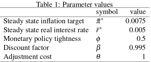
IRFs and simulations share the same non-shock parameters. The adjustment cost
pa-rameter, θ, equals 1. It represents the weight given to each part of equation (1), but also
determines persistence. There exists no prior for the parameter; 1 means both part of the
ob-jective function carries the same weight. The discount factor,β, equals 0.995 and ¯r∗ equals
1−β. For monetary policy, the steady state inflation target, ¯π∗, translates a 3 percent per year
inflation target, at 0.75 percent per quarter. The inflation target does not alter the results; a 3
percent target simply makes Figures3and4easier to read than the more common 2 percent
target.
Furthermore, the parameterφ shows what happens when the central bank reacts (φ=0.5)
or not (φ =0) to shocks. The choice of 0.5 for φ comes from inserting equation (3) into
equation (2),it=Et[rt∗+1+ (1+φ)πt+1−φ πt∗+1], yielding an influence of inflation on
nom-inal interest rate of 1.5, as in Taylor (1993). If φ =0, the long term part of equation (4),
Et
r∗
t+1+πt∗+1
, disappears and the private bank forever choose not to change nominal
in-terest rates. Inin-terestingly, that looks like the ancient equilibrium practice, where nominal
interest rates came more or less from tradition, so the market achieved changes in real
inter-4I used Dynare and Matlab(tm) to create the IRFs, simulations and figures, using the default seed so not to
Table 1: Parameter values
symbol value Steady state inflation target π¯∗ 0.0075
Steady state real interest rate r¯∗ 0.005
Monetary policy tightness φ 0.5 Discount factor β 0.995
Adjustment cost θ 1
est rates through inflation.
Table1lists the parameter values.
3.1
Impulse response functions
This subsection presents the implications of the model in terms of impact analysis. Results
from IRFs include: (1) a constant inflation target lowers real interest rate volatility
com-pared to no monetary policy intervention, (2) a moving inflation target raises volatility even
more, (3) persistent shocks have more effect on nominal interest rates, temporary shocks
on inflation and (4) anticipated real interest rate shocks lead to immediate response thereby
simulating the price puzzle. Furthermore, the results reinforce the intuition behind nominal
interest rate rigidity, as central banks need to move interest rates in the opposite direction
of where they want to move inflation (except when the inflation target changes) and credit
conditions cause inflation to be procyclical.
For IRFs, the persistence parameters for the shocks switch fromρ=0.75 for temporary
shocks toρ=0.999999 for permanent shocks (not exactly 1 to secure a numerical solution).
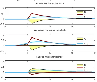
Figures1and2illustrate three possible outcomes for respectively temporary and
perma-nent positive one percent shocks. The three shocks of each figure consist of a surprise real
interest rate shock, an anticipated real interest rate shock and a surprise shock to the
infla-tion target. For an anticipated shock to the inflainfla-tion target, see Figure5 in the Appendix.
Figure 1: Temporary one percent shock responses
Surprise real interest rate shock
πt rt it−1
Anticipated real interest rate shock
πt rt it−1
Surprise inflation target shock
πt rt it−1
-5 0 5 10 15
-5 0 5 10 15
-5 0 5 10 15
-0.5 0 0.5 1 -0.5 0 0.5 1 -0.5 0 0.5 1
Note: the vertical axis represents the inflation rate (πt), the ex post real interest rate (rt) and the nominal interest
rate (it−1) in percent deviation from control state; the horizontal axis indicates quarters to or from the shock.
interest rates. The shocks appear in deviations from control levels.
In terms of interpretation, real interest shocks originate either from the real economy or
from the central bank trying to attain its target inflation rate. They illustrate shocks tor∗, but
also show the effects of monetary policy when inflation differs from its target.
The figures uncover three results. First, the inflation target shock means that real interest
rates increase in volatility if a central bank adopts a volatile inflation target. The next
subsec-tion provides further results for the monetary policy influence on real interest rates volatility.
Second, persistent shocks affect nominal interest rates more, while temporary shocks mostly
affect inflation. Third, anticipated shocks simulate the price puzzle.5 As we can see in the
figures for anticipated real interest rate shocks, rises in nominal interest rate and inflation
5Sims(1992) discovered the price puzzle, and described it as an empirical anomaly. It states that an increase
Figure 2: Permanent one percent shock responses
Surprise real interest rate shock
πt rt it−1
Anticipated real interest rate shock
πt rt it−1
Surprise inflation target shock
πt rt it−1
-5 0 5 10 15
-5 0 5 10 15
-5 0 5 10 15
-0.5 0 0.5 1 -0.5 0 0.5 1 -0.5 0 0.5 1
Note: the vertical axis represents the inflation rate (πt), the ex post real interest rate (rt) and the nominal interest
rate (it−1) in percent deviation from control state; the horizontal axis indicates quarters to or from the shock.
appear simultaneously some time before deflation sets in.
These results reinforce the intuition behind nominal interest rate rigidity. First, it shows
that, in the presence of rate rigidity, the Fisher effect is inverted in the short term. The
argument simply applies the Fisher equation (i=r+π). A rise in real interest rates can
either translate to a one to one rise in nominal interest rates, an inverse one to one drop in
inflation or a mix of the two. In the presence of rigidity, a rise in real interest rates cannot lead
to an equal rise in nominal interest rates, therefore leads to disinflation. Consequently, the
central bank’s operations do not directly lower nominal interest rates, but, in reality, yanks
down the real ones. In doing so, it creates inflation.
Second, the results imply that the relationship between economic fluctuations and
in-flation supports a relationship between credit conditions and fluctuations. The relationship
pres-ence of deflationary pressures in (say) ordinary recessions needs to come from an inverse
relation between real interest rates and production within the cyclical time frame.
The existence of a link between credit conditions, as a fuller characterization of
reces-sions, and of the 2008 recession in particular, emerged as a crucial subject of research. Such
is the case in other periods as shown, for example, byEckstein and Sinai(1986) or Ng and
Wright(2013). To quote Bernanke, Gertler and Gilchrist(1999, p. 1343): “First, it appears
that introducing credit-market frictions into the standard models can help improve their
abil-ity to explain even ‘garden-variety’ cyclical fluctuations.”
Furthermore, the predicting power of an inversion of the yield curve on recessions (see
Stock and Watson(1989), Adrian, Estrella and Hyun (2010) and Rudebusch and Williams
(2009)) also suggests credit crunches are a critical aspect of the business cycle. The yield
curve inverts when markets expect temporarily tight credit in the near future.
Of course, such a link does not predict a causal relationship, whether from production
to credit conditions in a financial accelerator type of argument, as inBernanke, Gertler and
Gilchrist(1996,1999) orKiyotaki and Moore(1997), or from credit conditions to production
in a credit cycle type of argument. Without clarifying the issue, this paper makes a strong
case for future research into the relationship between fluctuations and credit conditions. In
fact, the literature pertaining to credit conditions, whether of financial accelerator or credit
cycle flavors, is developing at a healthy pace.
3.2
Monetary regime simulations
Four different monetary regimes approximate interest rates data: a gold standard, a liquidity
trap, a non-target fiat and an inflation target regime. A volatile inflation target simulates
the gold standard and replicates the regime’s high volatility in ex post real interest rates.
I skipped the liquidity trap. A very persistent inflation target process simulates the
Table 2: Shock parameter values
standard deviation persistence Surprise real interest rate shock 0.005 0.6 Anticipated real interest rate shock 0.005 0.6 Inflation target shocks
... under gold standard regime 0.13 -0.05 ... under non-target fiat regime 0.004 0.975 ... under inflation target regime 0 10−8
persistent ex post real rates. For the inflation target regime, the target obviously does not
move. Overall, simulations show that inflation target schemes exist that can simulate how
most real and nominal interest rates behavior looks.
For all simulations, surprise and anticipated real-interest-rate shocks respectively follow
processes each with 0.6 persistence and standard deviations of 0.005. Table2lists the shock
parameter values applied to the regimes.
Table 3 compares the standard errors and correlation of nominal and real interest rates
for the data and the three regimes simulated. The small size of the annual sample for each
regime makes these results unreliable. Thus, the calibration efforts mostly concentrate on
showing what the model can do. A more thorough empirical investigation lies outside the
scope of an exposition paper.
The first part of Figure 3 shows data from Shiller (1989, Chapter 26) and updated by
him for one year nominal and ex post real interest rates. The other part of Figure 3 and
Figure4show simulations of the different monetary regimes for one year nominal and ex post
real interest rates. The figures present annualized simulation output in order to simulate the
averaging effect that yearly data produces. Figure6in the Appendix shows these simulations
Table 3: Standard deviations and correlation Simulations Data Gold Standard 1871-1931
r i r i
Standard deviation 8.07 1.09 8.34 1.16 Persistence 0.09 0.66 0.15 0.29
Correlation 0.39 0.48
Non-target Fiat 1965-1985
r i r i
Standard deviation 2.30 2.11 3.00 2.94 Persistence 0.32 0.95 0.68 0.59
Correlation 0.20 0.62
Inflation Target 1991-2011
r i r i
Standard deviation 1.99 0.96 1.92 1.43 Persistence 0.32 0.59 0.47 0.74
Correlation 0.83 0.65
Note: standard deviations in percent.
3.2.1 Gold standard regime
The first regime, before the Great Depression, corresponds to gold standard periods. It
rep-resents one regime. Different implementations do not show in rates data though monetary
authorities implemented the gold standard differently at different time in practice. The regime
displays a high volatility in ex post real interest rates and inflation, but a lower volatility in
nominal interest rates. The focus of the central bank on inflation, that started much later,
may explain the absence of the recent inflation persistence in this period. Inflation
persis-tence emerged as a stylized fact after World War II.
A volatile inflation target simulates the regime. This inflation target needs a large variance
to make the figures look right. Consequently, it follows a first-order autoregressive process
with a standard deviation of 0.13 and a persistence of -0.05. This supposes a large variance
in gold prices, coherent with gold prices still seen today.
Figure 3: Observed and simulated gold standard regime
Historical data
rt it−1
Gold standard simulations
rt it−1
20 40 60 80 100 120 140
1880 1900 1920 1940 1960 1980 2000
-10 0 10 20 -10 0 10 20
Note: the vertical axis represents the ex post real interest rate (rt) and the nominal interest rate (it−1) in percent;
the horizontal axis indicates years.
interest rate volatility and puts the Great Moderation in perspective.6 The model predicts
standard deviation of real interest rates under the gold standards at about four times that of
real interest rates under the inflation target regime.
3.2.2 Liquidity trap regime
The second regime, from the Great Depression to before the Bretton Woods system, saw
the economy going in and out of either a liquidity trap or severe financial repression. That
regime displays often negative ex post real interest rates and nominal interest rates near the
zero bound. Since the simulation model cannot deal with asymmetries caused by the zero
lower bound of nominal interest rates, I did not simulate the regime.
6Kim and Nelson(1999) andMcConnell and Perez-Quiros(2000) uncovered the Great Moderation, and
Figure 4: Simulated non-target fiat and inflation target regimes
Non-target fiat simulations
rt it−1
Inflation target simulations
rt it−1
20 40 60 80 100 120 140
20 40 60 80 100 120 140
-10 0 10 20 -10 0 10 20
Note: the vertical axis represents the ex post real interest rate (rt) and the nominal interest rate (it−1) in percent;
the horizontal axis indicates years.
Still, the model predicts a liquidity trap. If nominal interest rates hit the zero lower
bound, agents doubt the inflation target because the central bank cannot lower interest rates
to increase inflation. The private bank then chooses not to react to changes in real interest
rates or in the inflation target. It results in a long period of zero interest rates that only ends
when real interest rates descend under minus target inflation. In terms of policy, the model
therefore predicts that the economy can only get out of a liquidity trap through financial
repression or luck.
3.2.3 Non-target fiat regime
The third regime, the non-target fiat, starts with the Bretton Woods Agreement and ends
sometimes in the late eighties or early nineties. Though Bretton Woods officially implements
banks managed the inflation target globally. This regime seems plagued by non-stationarity.
Furthermore, unlike under the other regimes, sometimes real and nominal interest rates move
in visibly opposite directions. From the model’s perspective, as the IRFs showed, these
opposite moves signal changes in real rates prompted by changes in the inflation target.
For the postwar period until around the eighties, I determined that a persistent
infla-tion target process, of 0.975, best describes what was happening as inflainfla-tion went gradually
higher until Volker, and then went gradually down until the early nineties. The apparent
non-stationarity in the data pleads for the use of persistent shocks. Thus, the inflation target
follows a first-order autoregressive process with a standard deviation of 0.004 and a
persis-tence of 0.975.
The results from simulation of this regime show how persistence in inflation leads to high
persistence in nominal rates. Furthermore, real and nominal interest rates move sometimes
in opposite directions as found in the data.
Still, the simulation lacks a Volker moment, namely the moment when a sharp drop in
the inflation target lead to a sharp rise in real interest rates. In the simulation, changes in the
inflation target translate to almost equivalent changes in the nominal interest rate. Abrupt
changes in the inflation target only translate to abrupt changes in the real interest rate when
temporary, as in the Gold standard simulation. This may signal a failure not of the model,
but of the Fed’s credibility, as agents may have doubted the Fed’s resolve to keep inflation
low.
3.2.4 Inflation target regime
The last regime saw some form of inflation targeting scheme. Consistent with a persistent
inflation rate, both real and nominal interest rates seem to want to move in tandem. In this
regime, the inflation target stays constant.
ac-count for errors in predictions made by the central bank. Though a useful addition to a
projection model preoccupied with curve fitting, a small shock serves no purpose here.
As expected, the results show the annualized nominal and real rates tend to move in
tandem except when the real rate moves in a spike. In such a spike move, the nominal rate
will not completely follow.
3.2.5 Summary
Different inflation target processes can describe all three regimes: a volatile inflation target
for the gold standards, a less volatile, but more persistent target for the non-target fiat regime,
and a fixed target for the more recent regime. In terms of results, the variable inflation
tar-gets increase real interest rate volatility, persistent inflation tartar-gets lead to persistent nominal
interest rates, while a constant target leads to more stable real interest rates.
We can envision that inflation target schemes exist that can simulate how real and nominal
interest rates behavior looks. For lack of a thorough empirical investigation, we can say, at
the very least, that the model shows promise. The interest rate processes that emerge from
simulations appear realistic.
4
Conclusion
A large literature supports the central postulate that interest rate are rigid, as well as the
pro-cyclicality of inflation and how we believe monetary authorities use interest rates to
manip-ulate inflation. This paper looked at the macroeconomic implications of rigidity in nominal
interest rates.
In terms of results, an interest rate rigidity model of inflation emerges as a satisfactory
implementation of price evolution that could be used inside a larger macroeconomic model.
central banks move nominal interest rates in opposite direction to control inflation and why
credit conditions amid recessions lead to deflationary pressures. Side contributions include a
possible explanation of the price puzzle, from the preemptive aspect of nominal interest rate
setting, and of the Great Moderation, from the destabilizing effect of variable inflation target
policies prior to the mid-eighties.
Although the model displays realistic simulation results, the paper offers no estimation
of the model’s parameters or test of the theory. Issues related to identification and the choice
of data force estimation to be left for future research.
References
Adrian, Tiobias, Arturo Estrella and Song Shin Hyun (2010), “Monetary Cycles, Financial
Cycles, and the Business Cycle,”Staff report, Federal Reserve Bank of New York.
Benati, Luca (2008), “Investigating Inflation Persistence Across Monetary Regimes,” The
Quarterly Journal of Economics,123(3), pp. 1005–1060.
Benhabib, Jess, Stephanie Schmitt-Groh´e and Mart´ın Uribe (2001), “The Perils of Taylor
Rules,”Journal of Economic Theory,96(1-2), pp. 40–69.
Bernanke, Ben S., Mark Gertler and Simon Gilchrist (1996),“The Financial Accelerator and
the Flight to Quality,”Review of Economics and Statistics,78(1), pp. 1–15.
——— (1999),“The Financial Accelerator in a Quantitative Business Cycle Framework,”in
Handbook of Macroeconomics, eds. John B. Taylor and Michael Woodford, volume 1(C),
chapter 21, pp. 1341–1393, Amsterdam: Elsevier.
Carmichael, Jeffrey and Peter W. Stebbing (1983),“Fisher’s Paradox and the Theory of
In-terest,”American Economic Review,73(4), pp. 619–630.
Christiano, Lawrence J., Martin Eichenbaum and Charles L. Evans (2005),“Nominal
Rigidi-ties and the Dynamic Effects of a Shock to Monetary Policy,” Journal of Political
Econ-omy,113(1), pp. 1–45.
Clarida, Richard, Jordi Gal´ı and Mark Gertler (1998), “Monetary policy rules in practice:
Some international evidence,”European Economic Review,42(6), pp. 1033–1067.
Cochrane, John H. (2011),“Determinacy and Identification with Taylor Rules,” Journal of
Political Economy,119(3), pp. 565–615.
Craig, Ben R. and Valeriya Dinger (2014), “The Duration of Bank Retail Interest Rates,”
International Journal of the Economics of Business,21(2), pp. 191–207.
de Bondt, Gabe, Benoˆıt Mojon and Natacha Valla (2005),“Term structure and the
sluggish-ness of retail bank interest rates in euro area countries,” Working Paper Series, 518, pp.
1–49.
de Bondt, Gabe J. (2005), “Interest rate pass-through: empirical results for the euro area,”
German Economic Review,6(1), pp. 37–78.
Eckstein, Otto and Allen Sinai (1986),“The Mechanisms of the Business Cycle in the
Post-war Era,”inThe American Business Cycle: Continuity and Change, ed. Robert J. Gordon,
chapter 1, pp. 39–122, Cambridge: National Bureau of Economic Research.
Eichenbaum, Martin (1992), “Comments on ’Interpreting the macroeconomic time series
facts: The effects of monetary policy’ by Christopher Sims,”European Economic Review,
Illes, Anamaria and Marco Jacopo Lombardi (2013), “Interest rate pass-through since the
financial crisis,”BIS Quarterly Review,24(4), pp. 57–66.
Kim, Chang-Jin and Charles R. Nelson (1999),“Has the U.S. Economy Become More
Sta-ble? A Bayesian Approach Based on a Markov-Switching Model of the Business Cycle,”
Review of Economics and Statistics,81(4), pp. 608–616.
Kiyotaki, Nobuhiro and John Moore (1997),“Credit Cycles,” Journal of Political Economy,
105(2), pp. 211–248.
Klenow, Peter J. and Benjamin A. Malin (2010), “Microeconomic Evidence on
Price-Setting,”inHandbook of Monetary Economics, eds. Benjamin M. Friedman and Michael
Woodford, volume 3 ofHandbook of Monetary Economics, chapter 6, pp. 231–284,
Else-vier.
Kobayashi, Teruyoshi (2008), “Incomplete Interest Rate Pass-Through and Optimal
Mone-tary Policy,”International Journal of Central Banking,4(3), pp. 77–118.
McConnell, Margaret M. and Gabriel Perez-Quiros (2000), “Output Fluctuations in the
United States: What Has Changed since the Early 1980’s?” American Economic Review,
90(5), pp. 1464–1476.
Ng, Serena and Jonathan H. Wright (2013),“Facts and Challenges from the Great Recession
for Forecasting and Macroeconomic Modeling,” Journal of Economic Literature, 51(4),
pp. 1120–1154.
Ravenna, Federico and Carl E. Walsh (2006),“Optimal monetary policy with the cost
chan-nel,”Journal of Monetary Economics,53(2), pp. 199–216.
Rotemberg, Julio J (1982),“Sticky Prices in the United States,”Journal of Political Economy,
Rudebusch, Glenn D. and John C. Williams (2009), “Forecasting Recessions: The Puzzle
of the Enduring Power of the Yield Curve,” Journal of Business & Economic Statistics,
27(4), pp. 492–503.
Shiller, Robert J. (1989), Market Volatility, Princeton and Oxford: The MIT Press, data
available athttp://www.econ.yale.edu/∼shiller/data/chapt26.xls.
Sims, Christopher A. (1992),“Interpreting the macroeconomic time series facts: The effects
of monetary policy,”European Economic Review,36(5), pp. 975–1000.
Stock, James H. and Mark W. Watson (1989),“New Indices of Coincident and Leading
Indi-cators,”inNBER Macroeconomics Annual 1989, eds. Olivier Jean Blanchard and Stanley
Fischer, volume 4, pp. 351–409, Cambridge, MA: MIT Press.
——— (2003), “Has the Business Cycle Changed and Why?” in NBER Macroeconomics
Annual 2002, eds. Mark Gertler and Kenneth Rogoff, volume 17, pp. 159–230, MIT Press.
Taylor, John B. (1993),“Discretion versus policy rules in practice,”Carnegie-Rochester
Con-ference Series on Public Policy,39, pp. 195–214.
Williamson, Stephen D. (2014),“Scarce collateral, the term premium, and quantitative
eas-ing,”Working Papers 2014-008A, Federal Reserve Bank of St. Louis.
Woodford, Michael (2003a),Interest and Prices: Foundations of a Theory of Monetary
Pol-icy, Princeton and Oxford: Princeton University Press.
——— (2003b),“Optimal Interest-Rate Smoothing,”Review of Economic Studies,70(4), pp.
A
Supplemental material: For Online Publication
Figure 5: One percent inflation target shock responses
Anticipated temporary shock
πt rt it−1
Anticipated permanent shock
πt rt it−1
-5 0 5 10 15
-5 0 5 10 15
-0.5 0 0.5 1 -0.5 0 0.5 1
Note: the vertical axis represents the inflation rate (πt), the ex post real interest rate (rt) and the nominal interest
rate (it−1) in percent deviation from control state; the horizontal axis indicates quarters to or from the shock.
Figure5shows nominal and real interest rate, as well as the inflation response to
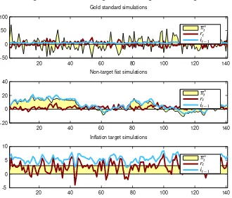
Figure 6: Simulated regimes showing inflation targets
Gold standard simulations
π∗
t rt it−1
Non-target fiat simulations
π∗
t rt it−1
Inflation target simulations
π∗
t rt it−1
20 40 60 80 100 120 140
20 40 60 80 100 120 140
20 40 60 80 100 120 140
-5 0 5 10 -20 0 20 40 -50 0 50 100
Note: the vertical axis represents the inflation target (π∗
t), the ex post real interest rate (rt) and the nominal
interest rate (it−1) in percent; the horizontal axis indicates years.
Figure6 shows annualized nominal and real interest rates, but also the inflation targets
Figure 7: Original 568 quarterly simulated periods
Gold standard simulations
π∗
t rt it−1
Non-target fiat simulations
π∗
t rt it−1
Inflation target simulations
π∗
t rt it−1
50 100 150 200 250 300 350 400 450 500 550 50 100 150 200 250 300 350 400 450 500 550 50 100 150 200 250 300 350 400 450 500 550
-2 0 2 4 -5 0 5 10 -50 0 50
Note: the vertical axis represents the inflation target (π∗
t), the ex post real interest rate (rt) and the nominal
interest rate (it−1) in percent; the horizontal axis indicates quarters.
Figure7shows the original quarterly nominal and real interest rates, as well as the