Nominal Income and Inflation Targeting
27
0
0
Full text
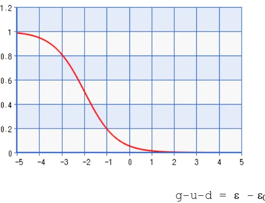
Figure

Related documents