Modeling and Current Programmed Control of a Bidirectional Full Bridge DC DC Converter

Modeling and Current Programmed Control of a

Bidirectional Full Bridge DC-DC Converter

Shahab H. A. Moghaddam, Ahmad Ayatollahi, Abdolreza Rahmati School of Electrical Engineering, Iran University of Science and Technology, Tehran, Iran

Email: [email protected], {ayatollahi, rahmati}@iust.ac.ir

Received February 7,2012; revised February 28, 2012; accepted March 16,2012

ABSTRACT

Modelling of bidirectional full bridge DC-DC converter as one of the most applicable converters has received signifi- cant attention. Mathematical modelling reduces the simulation time in comparison with detailed circuit response; moreover it is convenient for controller design purpose. Due to simple and effective methodology, average state space is the most common method among the modelling methods. In this paper a bidirectional full bridge converter is modelled by average state space andfor each mode of operations a controller is designed. Attained mathematical model results are in a close agreement with detailed circuit simulation.

Keywords: Average State Space; Bidirectional; Detailed Circuit Simulation; Full Bridge DC-DC Converter; Mathematical Modeling

1. Introduction

Modeling of DC-DC converter as one of the most appli- cable industrial converters has aroused a lot of interest. Since modeling gives us information about static and dynamic of the system, it is a crucial factor in design and control. Moreover, attained mathematical model can re- duce the simulation time in comparison with the simula-tion time provided by “cycle by cycle” solving the dif- ferential equations of the circuit, as is the case in matlab/ simulink.

With respect to renewable energy systems and optimum use of regenerated energy, interface converters should be capable of transferring power in both directions. So bidi- rectional DC-DC converters (BDC) are one of the most important interfaces that have applications such as: hybrid or electrical vehicles [1], aerospace systems [2], tele- communications, solar cells, battery chargers [3], DC motor drive circuits [4], uninterruptable power supplies [5-7], etc. so far many BDCs topologies have been in- troduced and surveyed [8,9]. In applications that trans- ferred power is more than 750 watts, full bridge topology is a proper one [10].

Bidirectional full bridge (FB) converters have been studied in many papers like [11-13]. A general modeling method that develops the discrete time average model is proposed in [12]. The operation period is divided to 3 intervals, the equivalent circuit and the differential equa- tions for each interval are written in matrix form. After solving equations and applying approximation of Taylor

expansion, the averaging state vector in half cycle gives us the final answer. Since time domain method employs numerical integration to solve differential equations the analysis is complicated and computationally intensive. Moreover the information about the dependence of the converter’s operating conditions on the circuit parameters is not provided [14].

modeling, average state space seems to be one of the most common, simplest, and effective methods, so in this paper we model a bidirectional full bridge DC-DC con- verter with average state space to gain the appropriate transfer functions for controller design purpose in both modes of operation.

2. Principle of Operation

Figure 1 shows the proposed bidirectional full bridge converter where arrows represent the direction of power flow. There are so many configurations for FB converters [11,14,24] with the same basic topology which differs from one another in the case of switching scheme or employing the elements of converter for the purpose of achieving ZVS or ZCS. Since modeling of this converter is the main purpose of this study and Changing modes of operation rely on conditions of application; these condi- tions are not taken into consideration.

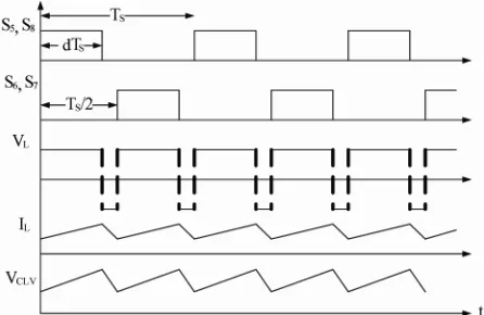
Detailed Circuit description can be reviewed in the lit- erature [24,25]. There are some long and short intervals in each mode, since the short ones are not as significant as long ones they can be left out. Meanwhile Figure 2 shows the basic waveforms and pulse gating of switches in boost mode operation, ignoring the short subintervals, Figure 3 depicts the buck mode waveforms. Small signal

Figure 1. Basic topology of the proposed FB bidirectional converter.

Figure 2. Ideal steady-state voltage and current waveforms of the converter in boost mode operation during one switch- ing cycle.

Figure 3. Ideal steady-state voltage and current waveforms of the converter in buck mode operation during one switch- ing cycle.

model of each mode will be extracted. For simplicity of control, gating circuit, and analysis, it is assume that in every mode only switches of one side are gated meanwhile the opposite ones are operating in their diode modes.

2.1. Boost Mode Operation

In boost mode with respect to pulse gating signals, there are two main intervals, consisting of four switches on and two diagonal switches on. When four switches turn on, input inductor voltage is equal to input source (low voltage side) and the inductor current increase pro- portional to the applied voltage. In this interval inductor saves the energy to transfer it in the next interval. While at the high voltage (HV) side the load is fed by the energy that has been transferred to the output filter (C) during pervious interval.

Next interval usually is known as the energy transfer interval. For instance, assume that S1 and S4 are on and

S2 and S3 are off. The input voltage plus inductor voltage

is applied to transformer and is scaled by n factor, ratio of secondary to primary voltage, then will be rectified through the other side of bridge. These processes will be repeated at next half switching cycle with this point that the primary applied voltage in next half switching cycle will be negative but will be rectified in the other side of the bridge.

2.2. Buck Mode Operation

With turning off the switches, next interval starts. Al- though the existence of leakage inductance prevents the switches go off immediately after applying gate turn off pulses and conduction of switches will continue through parasitic capacitors and diodes, but it is assumed that these subintervals are very short and can be neglected. In off time, the secondary side is only fed by the inductor stored energy, so the inductor current decreases propor- tional to output voltage. Next half switching cycle is the same, and only applied voltage of HV side is negative that is rectified in LV side.

3. Small Signal Modeling Using Average

State Space

Employing average state space method is divided into three phases:

1) With respect to switch conditions, the circuit is di- vided into different subintervals and state equations are written in the matrix form in each interval. State vectors are defined as inductors currents and capacitors voltages.

2) Averaged equations are formed by taking weighted average of state equations of each interval.

3) Averaged equations are written in differential form then linearization is done by perturbing variables. Em- ploying Laplace transform and omitting additional AC and DC terms (only first order AC terms), needed transfer functions are achieved.

For simplicity of modeling the following assumptions can be employed:

 Switches are ideal, there is no parasitic effect in switches;

 Inductor has no resistance;

 Transformer is ideal and there are no leakage and magnetizing inductances;

 Filter capacitors have low ESR (equivalent series re- sistance) that can be neglected;

 Load is constant and for modeling of the load change an additional current source has been added at the out- put;

 Each mode (buck or boost modes) starts with zero ini- tial condition.

State equations will be written in each mode separately and with some mathematical operations one can derive needed transfer functions.

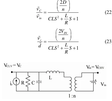
3.1. Boost Mode State Equations

As we saw in Section 2.1 in this mode two main intervals can be assumed. When all four switches conduct the equivalent circuit will be the same as shown in Figure 4 and the differential equations can be written as follows:

d d 1

d d

L L IN

v L  IN

i i

v

t t L (1)

d d 1 1

d d

c c c

z z C

v v v

C i i v

R t   t C RC (2)

d _{0 0} 1

0 d

1 ₁

d 0 ₀

d L L IN C Z c i i v t L v i v RC C t   _{ }     _{  }  _{ }     _{  }  _{ }    _{ }        _ _   (3)

This state lasts for (d – 0.5)Ts where s 1 s is

pe-riod of switching,

T  f

on s

dt T is the effective duty ratio

and n is turn ratio of secondary to primary windings. In the next interval when diagonal switches conduct, the equivalent circuit can be sketched as the same in Figure 5 and the state equations can be written as below:

d d 1 1

0

d d

C

L L

IN IN C

v

i i

v L v v

t n t L nL

       (4)

d d 1 1 1

d d

C C C L

Z L Z C

v v v

i

i c i i v

n  R  t  t nC C RC (5)

d 1 1

0 0

d

1

d 1 1 ₀

d L L IN C Z c i i v

t nL L

v i v C nC RC t    _       _{ }  _{ }      _{ }  _{ }   _{ }         _ _ _ _  









C Z

i v

Y v v Y

v i         _{ } _{ }     (6) (7)

This state lasts for (1 – d)Ts. The output state in both

intervals is the same as Equation (7). Now averaging the state equations during half switching cycle will result in the equation that has the characteristic of two intervals:

2( 1) 1

0 0

&

1

2(1 ) 1 ₀

t t d nL L A B d C nC RC                _      _ _   (8)

Figure 4. Equivalent circuit of boost mode operation with four LV switches on.

2( 1) 0

2(1 ) 1

L C C d nL i X d v nC RC   

   _{  } 1 0

1 0

L IN

Z

i _L v

v i C    _{  }         _{    }             





C Z v i    _{ }  

L L L

c C c

    _  _       (9)





i

Y CX DU

v  

   _{ }

  (10) Perturbing the state equations around their operating points will result in the equations that can be used for deriving the transfer functions; to do so one just need to write voltages and currents in the following forms:

IN IN in

Z z

i I

V V

v V

i

d D d

                         (11)









L

d d 2( 1)

d d

L L

C c

I D d

V

t t nL

 _{ }   _{  } (12)





_

_





C c z

D d I nC C V t t V RC  _                (13)





_

_

_

_

2 1 ₁

IN in D d V L d d L C c V t nL    _{ }         (14)









d c 2(1 ) 1 1

d L L C c z

D d

C C



I V

t nC  R  

   _{  }



 

  (15)

For extracting transfer functions additional AC and DC terms can be neglected. With applying Laplace trans- form to the equations one can achieve the following trans- fer functions.









2 1

4 1

c D n

S D

 

  



2 2 2

in _{n CLS n} L R

  (16)









2 8 1 2

4 1

2 2 2

L C IN

c nLI S D V nV

D           L

d _{n CLS n S}

R

 (17)









2 8 1

4 1

C L

L nCV S D I

S D

  



  



 _{2 2 2} L

d _{n CLS n} R

(18)





2

2

2 2 2 _{4 1}

c n SL

L S D    _{  }  _z

n CLS n R

(19)

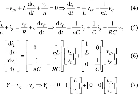
3.2. Buck Mode State Equations

The method is the same as mentioned in previous section for the boost mode operation. Two main operating inter- vals are considered to illustrate circuit conditions. No matter what switching scheme is employed, conventional PWM, phase shift or PWM plus phase shift, there is al- ways an effective duty cycle, Deff. Figures 6 and 7 depict

the main equivalent circuits meanwhile (20) and (21) describe state equations. Note that in writing equations, output voltage (LVS) is mentioned as Vc and the input

voltage at HV side is defined as Vin.

d 1 1

0 0

d

1 1

d ₀ 1

d L L IN C Z c i i v

t L nL

v i

v

C RC C

t    _       _{  }  _{ }      _{  }  _{ }   _{ }        _ _ _ _   (20)

This interval will lasts for dTs seconds. Following

in-terval will last for the remained half cycle, (0.5 – d)Ts.

d ₀ 1 1 ₀

d

1 1 1

d 0 d L L IN C Z c i i v

t L L

v i

v

C RC C

t    _       _{ }  _{ }      _{ }  _{ }   _{ }         _ _ _ _   (21)

Averaging in half switching cycle and perturbing the voltage and currents will result the needed transfer func-tions. 2 2 1 C in D n L CLS S R            

 (22)

2 2 1 IN c V n L

d _{CLS S}

R           

 (23)

Figure 6. Equivalent circuit of buck mode operation with two HV switches conducting.

2

2 2

1

IN _S VIN

n n

L S R

 _{ }

 

 

 

L

CV

d _CLS







 (24)

2 ₁

LS L

S R   

c z _CLS

  



 (25)

4. Model Verification

Having averaged state equation and perturbation one can achieve all transfer functions needed for controller design. In this section verification of the attained averaged model is done by comparing the step responses of transfer func-tions derived from average state space and simulated circuit in matlab/simulink.

4.1. Boost Mode

Start up process of open loop converter system with input voltage of 24 V is simulated under these conditions: D = 0.6, fs = 20 kHz, L = 200 μH, C = 50 μF, Vout = Vc = 300

V, Pin = Pout = 1.5 KW, R = 60 Ω.

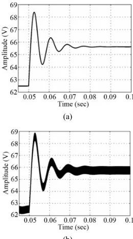
The simulated start up process of the predicted mathe- matical model and detailed circuit simulation with fixed duty cycle is depicted in Figures 8(a) and (b), respectively. Steady state, peak response, and rise time of output voltage in simulink is the same as obtained by the mathematical model but settling time differs 0.00007 seconds which is acceptable.

In order to check control to output and control to in- ductor current transfer functions, a small step (0.01) can

(a)

(b)

Figure 8. Start-up processes (a) Simulated mathematical

be applied to duty cycle in the both mathematical models and simulated circuit. Figure 9 shows the output voltage response to duty cycle change and Figure 10 represents the current waveforms while Figure 11 represents the out- put voltage change due to 1A step change in load cur- rent that is modeled by a current source, iz.

(a)

(b)

Figure 9. Output voltage in the presence of 0.01 step change in duty cycle. (a) Predicted response by mathematical averaged model; (b) Detailed circuit simulation in matlab/simulink.

(a)

(b)

(a)

(a)

(b)

Figure 11. Output voltage in presence of 1A step change

4.2. Buck Mode

open loop converter system with input

that the mathematical m

s (SMPS) control methodology

the

(b)

Figure 12. Open loop start u tput voltage with fixed duty in load current. (a) Predicted response by mathematical

averaged model; (b) Detailed circuit simulation in matlab/ simulink.

Start up process of

voltage of 300V is simulated under these conditions: D = 0.4, fs = 20 kHz, L = 200 μH, C = 50 μF, Vout = Vc = 24 V,

Pin = Pout = 1.5 KW, R = 0.384 Ω.

From Figure 12 it can be seen

odel has predicted the response of the converter very well. Figures 13 and 14 represent the behavior of output voltage and inductor current in the presence of 0.02 step change in duty cycle. Figure 15 shows converter output voltage due to 0.5A step change in load, it is obvious that the mathematical model is in a close agreement with simulated circuit.

5. Controller Design

can be divided into two main methods consisting of voltage mode control (VMC) and current mode control. Current mode control (CMC) is faster than voltage mode but it suffers from ringing, so merging two methods can cover the shortage of both. Current programmed control (CP) method that is presented in [10,26,27] employs CMC and VMC together. Figure 16 shows the block diagram of CPC which is mainly divided to peak, valley, and average [28]. Among all of those methods of CPC, the peak current programmed control (PCPC) is one of the most common modes and easiest one to understand.

p ou

cycle (a) predicted by mathematical model; (b) Detailed cir- cuit simulation with matlab/simulink.

(a)

(b)

(a)

Figure 16. Block diagram of peak current mode control

- r

(b)

Figure 14. Open loop respons inductor current e to 0.01 step change in duty cycle (a) predicted by mathematical

e of du

model; (b) Detailed circuit simulation with matlab/simulink.

(a)

(b)

Figure 15. Open loop respon utput voltage due to 1A step change load current (a) predicted by mathematical

se of o

model; (b) Detailed circuit simulation with matlab/simulink.

.

The method of PCMC modeling is the same as de sc ibed in [10], only up and down slopes and their times have been replaced to adapt the formulation with proposed topology. So the model of Figure 16 can be achieved, where Fm, Fin and Fc in boost and buck modes are deter-

mined in (26).





m c L in in c c

F F F

d       









3 4 boost mode

1

m a s

s in

s c

F

M T

D T

F

L

D T F

nL

 _

 

 

 _

 

 _

 



(26)





2 1

buck mode

1 4

m a s

s in

s c

F

M T

D T F

nL D T F

L

 _

 

 _

 

 

  

Not considering input voltage and load variations, the overall block diagram for both modes of operations can be depicted as Figure 17 with some algebraic operations; the loop gain transfer function of (27) can be concluded.

   

loop gain m V dc

c

F G H S G S

 (27)

1

c

m id m c V d

F G F F G 

 

Figure 17. Simplified block diagram of closed loop con- verter with neglecting the effect of line and load variation.

Figure 18. Uncompensated and compensated loop gain of boost mode solid line is uncompensated and dashed line is

efficients have been selected with spect to the method presented by Chien and Fruehauf

compensated response.

simple PID which its co re

[29].

 

 

 



_{ }







boost

G S F H S nLI S D V nV

T S    

den S 

 













2 2 2

2

2 2

4 1 8 1

C

mV

m L c

L

den S n CLS n nC F n

R

D D F I F V





  

     2

L m c

C m c IN

LI F F S

nF F V

 _ 

 

 



(28)



 



buck

G S F

T S

de

 ( ) 2

( )

IN H S nV

n S

 





2 2 2 ₂

2

m IN F V S 

(29)

m c IN

L

den S n CLS n nC

R

nF  R F V

 

 _  _

 

 

A simple integral controller can meet the

of buck mode compensating network. However, the de- signed controllers are not the optimum ones in terms of

ro

at the designed controllers are verter, they should be ex- ditional blocks like duty cycle

requirements

bustness. Other advanced control algorithms can be applied to this converter easily with the derived small signal model but that is beyond the scope of this work. Figure 19 represents uncompensated and compensated loop gain of buck mode.

6. Simulation Results In order to make sure th capable of controlling the con amined. In control loop ad

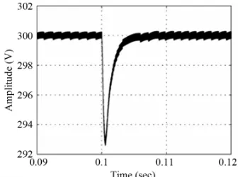
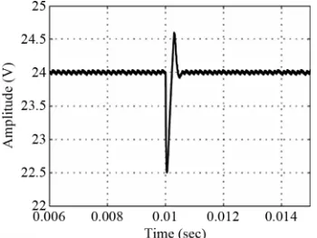
limiter are employed because at the start up there is no output voltage. This leads to 100% the duty cycle, as a result after some cycles; the circuit is gone to its steady state in which inductor and capacitor experience only a constant source and this is when they go under short and open circuit respectively. The other important block is compensating ramp which can overcome the unstable oscillation problem described in [10,22,30]. Figures 20 and 21 show that the controllers are successful to control the converter in the presence of 1 A and 10 A step load change for boost and buck mode respectively.

Figure 19. Uncompensated and compensated loop gain of buck mode, slid line is uncompensated and dashed line is compensated response.

Figure 21. Response of compensated closed loop circuit in buck mode operation in the presence of 5 A step load change.

7. Conclusion

In this paper a bidirectional full bridge DC-DC converter as one of the most applicable industrial converters has been modeled with average state space method. Sim tion results are in a close agreement with mathem model which approve the successfulness of average state space to predict the response. Current programmed con-troller was designed for each mode. Although compen-sated network was effective in buck mode but em l

requirements such as more bandwidth, phase margin and and load change rejection.

ula- atical

p oying modern and robust control algorithms can cope with the zero half plane problems in boost mode to achieve all the

capability of line

REFERENCES

[1] T. Mishima, E. Hiraki, T. Tanaka and M. Nakaoka, “A New Soft-Switched Bidirectional DC-DC Converter To- pology for Automotive High Voltage DC Bus Archi- tectures,” IEEE Vehicle Power and Propulsion Conference, Windsor, 6-8 September, 2006, pp. 1-6.

doi:10.1109/VPPC.2006.364281

[2] A. E. Navarro, P. Perol, E. J. Dede and F. J. Hurtado, “A New Efficiency Low Mass Bidirectional Battery Discharger-Charger Regulator for Low Voltage Batteries”, 27th Annual IEEE Power Electronics Specialists Confer- ence, Baveno, 23-27 June 1996, pp. 842-845.

doi:10.1109/PESC.1996.548679

[3] E.-S. Kim, K. -H.

Cho, “An Impr-Y. Joe, H.-Y. Choi, Y.-H. Kim and Y.oved Soft Switching Bi-Directional PSPWM FB DC/DC Converter,” Proceedings of the 24th Annual Conference of Industrial Electronics Society, Aachen, 31 August-4 September1998, pp. 740-743.

doi:10.1109/IECON.1998.724185 [4] H. L. Chan, K. W. E. Cheng and D. Suat

Square-Wave Converter with Bidirectional Power Flow,”anto, “A Novel Proceedings of the International Conference on Power Electronics and Drive Systems, Hohg Kong, 27-29 July 1999, pp. 966-971. doi:10.1109/PEDS.1999.792839 [5] M. Jain, P. K. Jain and M. Daniele, “Analysis of A Bi-

directional DC-DC Converter Topology for L Application,” IEEE Canadian C

ow Power onference on Electrical

and Computer Engineering, St. Johns, 25-28 May 1997, pp. 548-551. doi:10.1109/CCECE.1997.608283

[6] K. Venkatesan, “Current Mode Controlled Bideirectional Flyback Converter,” 20th Annual IEEE Power Electronics Specialists Conference,Milwaukee, 26-29 Ju

835-842.

ne 1989, pp. 8567

doi:10.1109/PESC.1989.4

[7] T. Reimann, S. Szeponik, G. Berger and J. Petzoldt, “A Novel Control Principle of Bidirectional DC-DC Power Conversion,” 28th Annual IEEE Power Electronics Spe- cialists Conference, St. Louis, 22-27 June 1997, pp. 978- 984. doi:10.1109/PESC.1997.616843

[8] M. K. Kazimierczuk, D. Q. Vuong, B. T. Nguyen and J. A. Weimer, “Topologies of Bidirectional PWM DC-DC Power Converter,” Proceedings of the IEEE National Aerospace and Electronics Conference, Dayton, 24-28 May 1993, pp. 435-441.

doi:10.1109/NAECON.1993.290953

[9] N. M. L. Tan, T. Abe and H. Akagi, “Topology and Ap- plication of Bidirectional Isolated DC-DC Converters,” IEEE 8th International Conference on Power Electronics and ECCE Asia, Jeju, 30 May-3 June 2011, pp. 1039- 1046. doi:10.1109/ICPE.2011.5944690

[10] R. W. Erickson and D. Maksimovic, “Fundamental of Power Electronics,” 2nd Edition, Kluwer Academic Pub- lishers,Alphen aan den Rijn, 2001.

[11] T. Mishima, E. Hiraki, T. Tanaka and M. Nakaoka, “High Frequency Link Symmetrical Active Edge Resonant Snubbers-Assisted ZCS-PWM DC-DC Converter,” Elec- tric Power Applications, Vol. 1, No. 6, 2007, pp. 907- 914. doi:10.1049/iet-epa:20060508

[12] C. Zhao, S. D. Round and J. W. Kolar, “Full-Order Aver- aging Modeling of Zero-Voltage Switching Phase-Shift Bidirectional DC-DC Converters,” Power Electronics, Vol. 3, No. 3, 2010, pp. 400-410.

doi:10.1049/iet-pel.2008.0208

[13] F. Krismer and J. W. Kolar, “Accurate Small-Signal Model for the Digital Control of an Automotive Bidirectional Dual Active Bridge,” IEEE Transactions on Power Elec- tronics,Vol. 24, No. 12, 2009, pp. 2756-2768.

doi:10.1109/TPEL.2009.2027904

[14] P. Jain and J. E. Quaicoe, “Generalized Modeling of Con- stant Frequency DC/DC Resonant Converter Topologies,” 14th International Telecommunications Energy Confer- ence, Washington DC, 4-8 October 1992, pp. 180-185. doi:10.1109/INTLEC.1992.268444

[15] L. A. Aguirre, P. F. Donoso-Garcia and R. Santos-Filho, “Use of a Priori Information in the Identification of Global Nonlinear Models—A Case

Converter,” IEEE Transactions

Study Using a Buck on Circuits and Systems I: Fundamental Theory and Applications, Vol. 47, No. 7, 2000, pp. 1081-1085. doi:10.1109/81.855463

[16] K. T. Chau and C. C. Chan, “Nonlinear Identification of Power Electronics Systems,” Proceedings of Inte

Conference on Power Electronics

rnational and Drive Systems, Singapore, 21-24 February 1995, pp. 329-334.

doi:10.1109/PEDS.1995.404900

Power Electronics,Vol. 22, No. 4, 2007, pp. 1210-1221. doi:10.1109/TPEL.2007.900551

[18] F. Alonge, F. D’Ippolito and T. Cangemi, “Hammerstein Model-Based Robust Control of DC/DC Converters,” 7th International Conference on Power Electronics and Drive Systems, Bangkok, 27-30 November 2007, pp. 754-762. doi:10.1109/PEDS.2007.4487788

[19] V. Vorperian, R. Tymerski and F. C. Lee, “Equivalent Circuit Model for Resonant and PWM Switches,” IEEE Transactions on Power Electronics, Vol. 4, No.

pp. 205-214.

2, 1989, doi:10.1109/63.24905

[20] V. Vorperian, “Simplified Analysis of PWM Converter Using the Model of the PWM Switch: part I and II,” IEEE Transactions on Aerospace and Electronic Systems, Vol. 26, No. 3, 1990, pp. 497-505. doi:10.1109/7.106127 [21] R. D. Middlebrook and S. Cuk, “A General Unified Ap-

proach to Modeling Switching Converter Power Stages,” International Journal of Electronics,Vol. 42, No. 6, 1977, pp. 521-550. doi:10.1080/00207217708900678

[22] S.-P. Hsu, A. Brown, L. Rensink and R. D. Middle-Brook, “Modeling and Analysis of Switching DC-to-DC Con- verters in Constant-Frequency Current Programmed Mode”, Power Electronics Specialists Conference, San Diego, 18-22 June 1979, pp. 284-301.

[23] S. Cuk, “Modeling, Analysis, and Design of Switching Converters,” Ph.D. Thesis, California Institute of Tech- nology, Pasadena, 1976.

[24] L. Zhu, “A Novel Soft-Commutating Isolated Boost Full-Bridge ZVS-PWM DC-DC Converter for Bidirec-

tional High Power Applications,” IEEE Transactions on Power Electronics, Vol. 21, No. 2, 2004, pp. 422-429. doi:10.1109/TPEL.2005.869730

[25] R. Li , A. Pottharst, N. Frohleke and J. Bocker, “Analysis and Design of Improved Isolated Full-Bridge Bidirec- tional DC-DC Converter,” 35th Annual Power Electronics Specialists Conference, Aachen, 20-25 June 2004, pp. 521- 526. doi:10.1109/PESC.2004.1355801

[26] R. B. Ridley, “A New, Continuous-Time Model for Cur rent Mode Control,” IEEE Trans

- actions on Power Elec- tronics, Vol. 6, No. 2, 1991, pp. 271-280.

doi:10.1109/63.76813

[27] L. Peng and B. Lehman, “A Design Method for Parallel- ing Current Mode Controlled DC-DC Converters,” IEEE Transactions on Power Electronics, Vol. 19, No. 3, 2004, pp 748-756. doi:10.1109/TPEL.2004.826497

[28] R. Sheehan, “Understanding and Applying Current-Mode Control Theory,” Power Electronics Techn

tion and Conference, Da

ology Exhibi- llas, 30 October-1 November,2007, pp. 1-26.

[29] D. E. Seborg, T. F. Edgar and D. A. Millichamp, “Process Dynamics and Control,” 2nd Edition, John Wiley and Sons Inc., New York, 2004.