Comparison of RANS and LES in the Prediction of Airflow Field over Steep Complex Terrain

ISSN Online: 2165-3860 ISSN Print: 2165-3852

DOI: 10.4236/ojfd.2018.83018 Sep. 3, 2018 286 Open Journal of Fluid Dynamics

Comparison of RANS and LES in the Prediction

of Airflow Field over Steep Complex Terrain

Takanori Uchida

_{, Graham Li}

1_{Research Institute for Applied Mechanics (RIAM), Kyushu University, Fukuoka, Japan} 2_{Tsubasa Windfarm Design, Tokyo, Japan}

Abstract

The present study compared the prediction accuracy of the three CFD soft-ware packages for simulating airflow around a three-dimensional, isolated hill with a steep slope: 1) WindSim (turbulence model: RNG k-ε RANS), 2) Me-teodyn WT (turbulence model: k-L RANS), which are the leading commer-cially available CFD software packages in the wind power industry and 3) RIAM-COMPACT (turbulence model: standard Smagorinsky LES), which has been developed by the lead author of the present paper. Distinct differ-ences in the airflow patterns were identified in the vicinity of the isolated hill (especially downstream of the hill) between the RANS results and the LES results. No reverse flow region (vortex region) characterized by negative wind velocities was identified downstream of the isolated hill in the result from the simulation with WindSim (RNG k-ε RANS) and Meteodyn WT (k-L RANS). In the case of the simulation with RIAM-COMPACT natural terrain version (standard Smagorinsky LES), a reverse flow region (vortex region) characte-rized by negative wind velocities clearly forms. Next, an example of wind risk (terrain-induced turbulence) diagnostics was presented for a large-scale wind farm in China. The vertical profiles of the streamwise (x) wind velocity do not follow the so-called power law wind profile; a large velocity deficit can be seen between the hub center and the lower end of the swept area in the case of the LES calculation (RIAM-COMPACT).

Keywords

RANS, LES, Isolated Hill, Large-Scale Wind Farm

1. Introduction

We have developed an unsteady and non-linear wind synopsis simulator called RIAM-COMPACT (Research Institute for Applied Mechanics, Kyushu

Univer-How to cite this paper: Uchida, T. and Li, G. (2018) Comparison of RANS and LES in the Prediction of Airflow Field over Steep Complex Terrain. Open Journal of Fluid Dynamics, 8, 286-307.

https://doi.org/10.4236/ojfd.2018.83018

Received: November 13, 2017 Accepted: August 31, 2018 Published: September 3, 2018

Copyright © 2018 by authors and Scientific Research Publishing Inc. This work is licensed under the Creative Commons Attribution International License (CC BY 4.0).

DOI: 10.4236/ojfd.2018.83018 287 Open Journal of Fluid Dynamics sity, Computational Prediction of Airflow over Complex Terrain) in order to simulate the airflow on a microscale, i.e., a few tens of km or less [1]-[13]. In RIAM-COMPACT, a large-eddy simulation (LES) has been adopted for turbu-lence modeling. LES is a technique in which the structures of relatively large ed-dies are directly simulated and smaller eded-dies are modeled using a sub-grid scale model. Efforts have been made to promote RIAM-COMPACT, mainly in the wind power industry (e.g., private wind power providers, local governments, and wind turbine manufacturers) in Japan. Computation time had been an issue of concern for the RIAM-COMPACT software, which focuses on unsteady turbu-lence simulations (LES). The present fluid simulation solver is compatible with multi-core CPUs such as the Intel Core i9 and also with GPGPU, which has drastically reduced the computation time, leaving no appreciable problems in terms of the practical use of the RIAM-COMPACT software.

On another front, commercially available CFD software such as STAR-CCM+ [14] and ANSYS (CFD, Fluent, CFX) [15] has developed mainly as an engineer-ing tool primarily in the automobile and aviation industries until the present time. Recently, some of the above-mentioned general purpose thermal fluid analysis software has started being adopted in the wind power industry. In the previous study [16] [17] [18], the simulation results obtained from the RIAM-COMPACT software were compared to those from STAR-CCM+, one of the leading commercially available CFD software packages. The results of the comparison are discussed. In addition, open-source CFD software packages are more widely used than in the past. One of the most widely used software pack-ages is OpenFOAM (OpenField Operation And Manipulation) [19]. Open-FOAM is an open-source CFD toolbox which has been released and distributed under the GNU GPL (General Public License) [20] by the OpenFOAM Founda-tion, a non-profit organization. In the previous study [21], the simulation results obtained from the RIAM-COMPACT software were also compared to those from OpenFOAM, and the results of the comparison are discussed.

DOI: 10.4236/ojfd.2018.83018 288 Open Journal of Fluid Dynamics In the present study, numerical simulations are performed for airflow over and around a three-dimensional, isolated hill with a steep slope angle using the three CFD software packages (WindSim, Meteodyn WT and RIAM-COMPACT). The results of the comparison are discussed. Next, the numerical simulations for airflow over a large-scale wind farm in China [21] are performed with RIAM-COMPACT, which is based on an LES turbulence model, and Meteodyn WT, which is based on a RANS turbulence model.

2. Overview of the Software Packages (RIAM-COMPACT and

WindSim) and Numerical Simulation Set-Up in the Case of

a Three-Dimensional, Isolated Hill with a Steep Slope

Angle

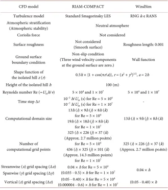
The numerical wind simulations in the present study are conducted for high Reynolds number airflow over and around a three-dimensional, isolated hill with a steep slope angle and a large-scale wind farm in China. Table 1 shows the simulation set-ups adopted in the two software packages which are used in

Table 1. Comparison of numerical simulation methods, parameters, and settings between the two software packages.

CFD model RIAM-COMPACT WindSim

Turbulence model Standard Smagorinsky LES RNG k-ε RANS

Atmospheric stratification

(Atmospheric stability) Neutral atmosphere

Coriolis force Not considered

Surface roughness _{(Smooth surface)} Not considered Roughness length: 0.001

Ground surface boundary condition

Non-slip condition (Three wind velocity components

at the ground surface are zero.) Wall function

Shape function of

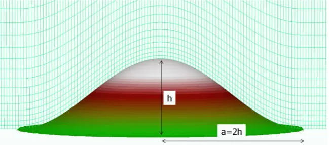
the isolated hill z (r) 0.5h × {1 + cos(πr/a)}, r = (x2 + y2)1/2, a = 2h

Height of the isolated hill h 100 (m)

Reynolds number Re (=Uinh/ν) 5 × 104 and 1 × 107 5 × 104 and 1 × 107

Time step Δt 10−3 h/Uin (s) for Re = 5 × 104

10−7 _h/U

in (s) for Re = 1 × 107 -

Computational domain size

13h (i) × 9h (j) × 8h (k) for Re = 5 × 104

13h (i) × 9h (j) × 8h (k) 19h (i) × 18h (j) × 8h (k)

for Re = 1 × 107

Number of computational grid points

325 (i) × 226 (j) × 37 (k) (Approx. 2.7 million points)

for Re = 5 × 104 _{325 (i) × 226 (j) × 37 (k)}

(Approx. 2.7 million points) 436 (i) × 325 (j) × 101 (k)

(Approx. 14.3 million points) for Re = 1 × 107

Streamwise (x) grid spacing (Δx) 0.04 × h for Re = 5 × 104

(0.035 - 0.5) × h for Re = 1 × 107 0.04 × h

Spanwise (y) grid spacing (Δy)

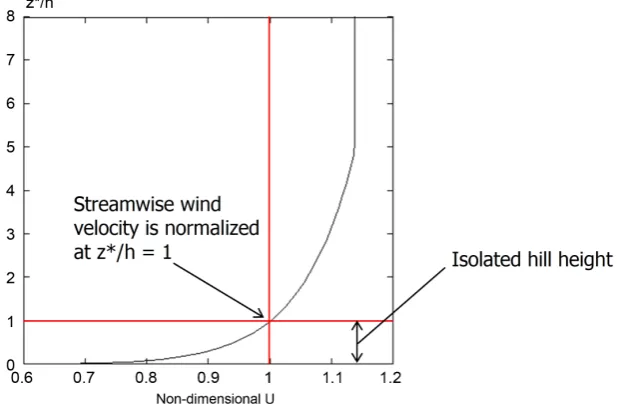
DOI: 10.4236/ojfd.2018.83018 289 Open Journal of Fluid Dynamics the present study: RIAM-COMPACT natural terrain version (turbulence model: LES) and WindSim (turbulence model: RANS). Figure 1 and Figure 2 illustrate the full computational grid used for WindSim and an enlarged view of the grid in the vicinity of the isolated hill, respectively. Figure 3 shows the inflow profile used for all of the simulations in the present study. Figure 4 shows the characte-ristic wind velocity and length scales which are employed for the simulations with RIAM-COMPACT.

In RIAM-COMPACT, a collocated grid in a general curvilinear coordinate system is used in order to numerically predict local wind flow over complex ter-rain with high accuracy while avoiding numerical instability. For the numerical simulation method, a FDM is adopted, and an LES model is used for the turbu-lence model. For the computational algorithm, a method similar to a FS method [24] is used, and a time marching method based on the Euler explicit method is adopted. The Poisson’s equation for pressure is solved by the SOR method.

Figure 1. Computational grid used in the simulations with WindSim, Re = 5 × 104 _{and 5}

× 107_.

DOI: 10.4236/ojfd.2018.83018 290 Open Journal of Fluid Dynamics Figure 3. Inflow wind velocity profile used in the present study.

Figure 4. Characteristic wind velocity and length scales used in the simulation with RIAM-COMPACT.

For discretization of all the spatial terms in the governing equations except for the convective term in the Navier-Stokes equation, a second-order central dif-ference scheme is applied. For the convective term, a third-order upwind differ-ence scheme is used. An interpolation technique based on four-point differenc-ing and four-point interpolation by Kajishima [25] is used for the fourth-order central differencing that appears in the discretized form of the convective term. For the weighting of the numerical diffusion term in the convective term discre-tized by third-order upwind differencing, α = 3.0 is commonly applied in the Kawamura-Kuwahara scheme [26]. However, α = 0.5 is used in the present study to minimize the influence of numerical diffusion. For the LES subgrid-scale modeling, the standard Smagorinsky model [27] is adopted with a model coeffi-cient of 0.1 in conjunction with a wall-damping function. For further details of the numerical simulation techniques, refer to Uchida [1]-[13].

DOI: 10.4236/ojfd.2018.83018 291 Open Journal of Fluid Dynamics are applied at the outflow boundary. On the ground surface, a non-slip boun-dary condition is imposed. For the simulation at Re (=Uinh/ν) = 107, the number of grid points is changed to 101 in the vertical direction, and the minimum ver-tical grid spacing in is set to Δzmin/h = 4 × 10−7 according to the equation below (see Table 1):

min

0.1 Re

z h

∆ = (1)

In contrast to RIAM-COMPACT, WindSim uses RANS models. In the present study, the RNG k-ε RANS model is selected for the simulations. Refer to [23] for the numerical simulation methods used in WindSim and other details about this software.

3. Comparison of the Simulation Results from the Two CFD

Software Packages (RIAM-COMPACT and WindSim) in the

Case of a Three-Dimensional, Isolated Hill with a Steep

Slope Angle

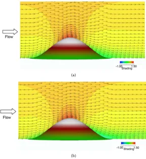
Figure 5 shows the ensemble-averaged flow fields from the simulations with WindSim (turbulence model: RNG k-ε RANS). In neither of these simulations

(a)

(b)

Figure 5. Wind velocity vectors and contour of streamwise (x) wind velocity (non-dimensional) on the x-z cross-section at the center of the span (y = 0), ensem-ble-averaged flow field, WindSim (turbulence model: RNG k-ε RANS).(a) Re = 5 × 104_;

DOI: 10.4236/ojfd.2018.83018 292 Open Journal of Fluid Dynamics (Re = 5 × 104 _{and 5 × 10}7_{) did a reverse flow region (vortex region), in which the} values of the streamwise wind velocity are negative, form downstream of the isolated hill. Instead, a potential-flow-like pattern formed in both simulations.

Figure 6 shows instantaneous flow fields from the simulations with RIAM-COMPACT (turbulence model: standard Smagorinsky LES) (Re = 5 × 104 and 1 × 107_{). An examination of these simulation results reveals the clear} pres-ence of a reverse flow region (vortex region), in which the values of the stream-wise wind velocity are negative, downstream of the isolated hill.

(a)

(b)

Figure 6. Wind velocity vectors and contour of streamwise (x) wind velocity (non-dimensional) on the x-z cross-section at the center of the span (y = 0), instantane-ous flow field, RIAM-COMPACT (turbulence model: standard Smagorinsky LES). (a) Re = 5 × 104_{, non-dimensional time = 5.0; (b) Re = 1 × 10}7_{, non-dimensional time = 7.0.}

4. Overview of the Software Packages (RIAM-COMPACT and

Meteodyn WT) and Numerical Simulation Set-Up in the

Case of a Three-Dimensional, Isolated Hill with a Steep

Slope Angle

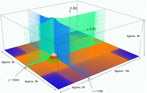
DOI: 10.4236/ojfd.2018.83018 293 Open Journal of Fluid Dynamics Meteodyn WT, which is based on a RANS turbulence model (see Table 2). Fig-ure 7 shows the computational domain and grid used for the simulation with Meteodyn WT. An enlarged view of the computational grid in the vicinity of the isolated hill from the simulation with Meteodyn WT is shown in Figure 8. Fig-ure 9 shows the method used to set the inflow profile in Meteodyn WT and the inflow profile generated for the present study.

Figure 7. Computational domain and grid used for the simulation with Meteodyn WT, Re = 107_.

Table 2. Comparison of numerical simulation methods, parameters, and settings between the two software packages.

CFD model RIAM-COMPACT Meteodyn WT

Turbulence model _{Smagorinsky LES} Standard _{(A single equation model)} k-L RANS

Atmospheric stratification

(Atmospheric stability) Neutral atmosphere

Coriolis force Not considered

Surface roughness _{(Smooth surface)} Not considered (For the ground surface not Roughness length: 0.05 on the isolated hill: 0.001)

Ground surface boundary condition

Non-slip condition (Three wind velocity components

at the ground surface are zero.) Shape function of the isolated hill z (r) 0.5h × {1 + cos(πr/a)} r = (x2 _{+ y}2_{)1/2, a = 2h}

Height of the isolated hill h 100 (m)

Reynolds number Re (=Uinh/ν) 106 107

Time step Δt 10−5 _h/U

in (s) -

Computational domain size 19h (i) × 18h (j) × 8h (k)

Number of computational grid points 436 (i) × 325 (j) × 101 (k) _{(Approx. 14.3 million points) (Approx. 5.2 million points)} 436 (i) × 325 (j) × 37 (k)

Streamwise (x) grid spacing (Δx)

(0.035 - 0.5) × h Spanwise (y) grid spacing (Δy)

DOI: 10.4236/ojfd.2018.83018 294 Open Journal of Fluid Dynamics Figure 8. Enlarged view of the computational grid used in the simulations with Meteodyn WT, Re = 107_.

Figure 9. Method adopted in Meteodyn WT for setting the inflow profile and the inflow profile generated for the present study.

Since simulations for a flow with Re (=Uinh/ν) = 107 were not feasible with the RIAM-COMPACT natural terrain version software because of the time step, a numerical wind simulation is performed at Re = 106_{, which is an order of} mag-nitude smaller than the flow simulated with Meteodyn WT. For this simulation, the number of grid points in the vertical direction is set to 101 (37 for the simu-lation with Meteodyn WT), and the minimum vertical spacing is set to Δzmin/h = 10−4 _{based on the Equation (1) (Δz}

min/h = 5.0 × 10−3 for the simulation with Me-teodyn WT, see Table 2). At the inflow boundary, an inflow profile which is al-most identical to the inflow profile used for the simulation with Meteodyn (Figure 9) is used. Free-slip conditions are applied at the side and upper boun-daries, and convective outflow conditions are applied at the outflow boundary. At the surfaces of the ground and the isolated hill, non-slip conditions are im-posed. The time step is set to Δt = 10−5_h/U

DOI: 10.4236/ojfd.2018.83018 295 Open Journal of Fluid Dynamics

5. Comparison of the Simulation Results from the Two CFD

Software Packages (RIAM-COMPACT and Meteodyn WT)

in the Case of a Three-Dimensional, Isolated Hill with a

Steep Slope Angle

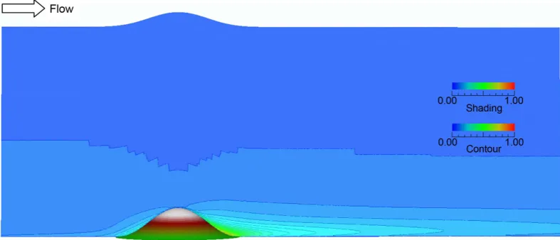
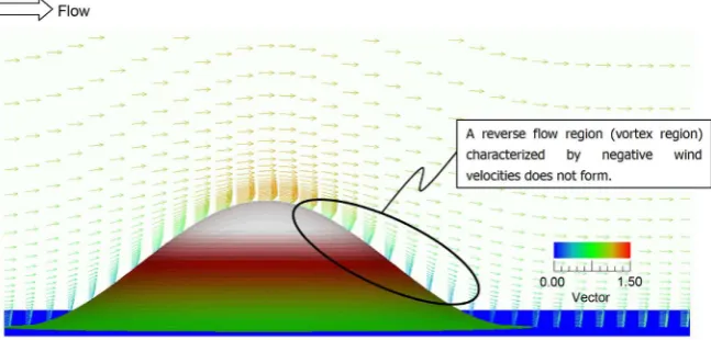
Figures 10-12 show results from the simulation with the Meteodyn WT soft-ware package (turbulence model: k-L RANS). These results (for a flow at Re = 107_{) indicate that a reverse flow region (vortex region) characterized by negative} values of wind velocity does not form downstream of the isolated hill, and a pat-tern resembling potential flow is present there. Figure 13 shows the results from the simulation with the RIAM-COMPACT natural terrain version software package (turbulence model: the standard Smagorinsky LES). Examinations of the results reveal that a reverse flow region (vortex region) characterized by neg-ative values of wind velocities clearly exists downstream of the isolated hill in the simulated flow at Re (=Uinh/ν) = 106.

Figure 10. Streamwise (x) wind velocity distribution at the center of the span (y = 0), Meteodyn WT, k-L RANS, Re = 107_.

DOI: 10.4236/ojfd.2018.83018 296 Open Journal of Fluid Dynamics Figure 12. Velocity vectors at the center of the span (y = 0) in the vicinity of the isolated hill, Meteodyn WT,k-L RANS model, Re = 107_.

Figure 13. Streamwise (x) wind velocity distribution at the center of the span (y = 0) in the vicinity of the isolated hill, RIAM-COMPACT, standard Smagorinsky LES, Re = 106_.

(a) Instantaneous flow field; (b) Time-averaged flow field.

6. Comparison of the Simulation Results from the Two CFD

Software Packages (RIAM-COMPACT and Meteodyn WT)

in the Case of a Large-Scale Wind Farm in China

DOI: 10.4236/ojfd.2018.83018 297 Open Journal of Fluid Dynamics

(a)

(b)

Figure 14. Large-scale wind farm investigated in the present study (Duogu Wind Farm). (a) Overall view; (b) Enlarged view. A group of 33 wind turbines are located above a steep escarpment.

ranges from around 1850 to 2200 meters. The cliff has a height of around 900 m with slopes exceeding 60 degrees in places. Aerial photos from Google Earth in-dicate vegetation is abundant at the bottom of the cliff but scarce along the cliff and in the vicinity of turbines. Since the start of operations, one of the wind tur-bines, turbine No.12 (T12) has experienced vibration problems. Wind farm op-erator Yunnan Huadian Dougu Wind Power Corporation (YUDWPC) sus-pected the vibration issue is related to wind conditions. In the present study, the simulations are performed with RIAM-COMPACT, which is based on an LES turbulence model, and WindSim, which is based on a RANS turbulence model. The results from the simulations are compared.

DOI: 10.4236/ojfd.2018.83018 298 Open Journal of Fluid Dynamics YUDWPC and a report was issued in April 2014 [28]. Stated in the report was that high vibration data was recorded only when the wind was blowing from the southwest. Wind direction on the ground level was observed to be in the reverse direction from that recorded by the nacelle anemometer. Analysis of the vibra-tion data indicates the vibravibra-tion is in the vertical direcvibra-tion. This suggests the vi-bration is associated with abnormal vertical wind shear across the wind turbine rotor. As shown in Figure 15, a figure extracted from the report, it was deduced that the presence of the small hill located about 150 m upstream from turbine T12 was causing the onset of turbulence and reverse flow which led to the vibra-tion recorded.

For LES simulation, the RIAM-COMPACT natural terrain version software package was employed. The software uses a standard Smagorinsky turbulence model. For the simulation, SRTM 90 m data was used for elevation data. Wind direction is set to true north at 247 degrees and the computational domain con-structed is shown in Figure 16 with the following details:

Figure 15. Deduction made on the airflow upstream and in the vicinity of turbine T12.

DOI: 10.4236/ojfd.2018.83018 299 Open Journal of Fluid Dynamics − Domain size: 14.0 km × 13.3 km × 8.3 km

− Elevation: 1275 m (Min) - 2232 m (Max) − Calculation grid points: 300 × 400 × 60 − Total number of grid points: 7.2 million

− Grid spacing: 8 m - 957 m (x), 13 m - 72 m (y), 1 m - 470 m (z)

To increase calculation accuracy, the mesh is concentrated around the turbine positions in both the x and y direction as shown in Figure 16. No roughness consideration is given inthe present LES simulation. Atmospheric stability is set to neutral stability. After the calculation has been stabilized, numerical results in the calculation domain are output for a real time of ten minutes with an interval of one second.

Figure 17 shows an instantaneous vector plot across turbine T12. This picture clearly shows flow separation occurred at the small hill located 140 m upstream from the turbine, and the onset of the formation of the recirculating vortex be-hind the hill. The turbulent flow extends downstream forming a reverse flow re-gion characterized by negative values of wind speed covering the lower part of the wind turbine rotor.

The simulation results also indicate that the wind flow is relatively undis-turbed above hub height level. The U component wind speed time series during the ten minute simulation at rotor top (106.3 m), hub center (65 m), rotor bot-tom (23.7 m) and surface level (10 m) positions are plotted in Figure 18.

Referring to Figure 18, it is obvious that the wind speed at surface (10 m) and rotor bottom is significantly lower and showing more fluctuations than the wind speed at the hub and top part of the rotor. Wind speed varies between 15.0 to 20.0 m/s at hub height and rotor top whereas for rotor bottom wind speed fluc-tuates between negative 6.2 m/s to 2.0 m/s. Negative wind speed indicates the

DOI: 10.4236/ojfd.2018.83018 300 Open Journal of Fluid Dynamics Figure 18. Time series of U component wind speed at rotor top, hub, rotor bottom and ground surface level at turbine T12.

wind is flowing in reverse direction. During the ten minute simulation, negative values account for 62% of the total data at rotor bottom. When the rotor bottom wind speed is at its minimum of negative 6.2 m/s the wind speed at rotor top is at 18.1 m/s, hence a very large absolute wind speed difference of 24.3 m/s. Excluding the negative wind speed data, the wind speed difference across the rotor face (be-tween rotor top and rotor bottom) has a maximum value of 18.7 m/s and an aver-age of 17.4 m/s. The maximum wind shear exponent is calculated to be 5.8 with an average value of 2.5, far exceeding the IEC standard average shear value of 0.2.

The average, minimum and maximum values of the U component wind speed at turbine T12 are shown in Figure 19. The average values represent the average shear profile seen at turbine T12. Referring to that, the reverse flow region re-sults in a negative or very low wind speed from ground surface level to the rotor bottom of around 25 m. Wind speed increases gradually from 25 m and starts leveling off at around 50 m.

In this study, the commercial software Meteodyn WT (turbulence model: k-L

DOI: 10.4236/ojfd.2018.83018 301 Open Journal of Fluid Dynamics Figure 19. Vertical shear profile predicted by RIAM-COMAPCT, average, minimum and maximum of U component wind speed variation with height.

Table 3. Numerical simulation methods, parameters, and settings for Meteodyn WT.

Wind direction 247 degrees

Thermal stability class 2

Smoothing-Whole domain 1

Forest model Robust model

Minimum horizontal spacing 5 m

Minimum vertical spacing 2 m

Horizontal expansion coefficient 1.1

Vertical expansion coefficient 1.2

Grid points _{(Approx. 2.3 million points)} 225 (i) × 237 (j) × 44 (k)

Maximum iteration number 25

Convergence 99.3 %

DOI: 10.4236/ojfd.2018.83018 302 Open Journal of Fluid Dynamics Table 4. Speed-up factor at turbine T12 and calculated wind speed.

Height (m) Speed-up factor Wind speed (m/s)

20 1.850 17.58

40 1.952 18.54

60 2.002 19.02

80 2.013 19.12

100 2.008 19.08

120 1.998 18.98

140 1.987 18.88

160 1.977 18.78

180 1.968 18.70

200 1.959 18.61

speed at different heights can be calculated based on the speed-up factor and the results are shown in Table 4.

The wind speed figures in Table 4 are plotted in Figure 20 and the resulting wind shear profile is compared with the shear profile (average values) predicted by RIAM-COMPACT. It can be seen from Figure 20 that the shapes of the two profiles are similar from 50 m upwards but distinctively different below 50 m. Meteodyn WT does not seem to predict any flow separation and reverse flow re-gion and therefore there is no significant wind speed reduction between 25 m and 50 m, and also no negative wind speed values below 25 m as predicted by RIAM-COMPACT. Numerical comparison results are shown in Table 5.

Referring to Table 5, across the wind turbine rotor face, RIAM-COMPACT predicted a large wind speed difference with a shear exponent exceeding the IEC standard value of 0.2 by a large margin. In sharp contrast, Meteodyn WT pre-dicted a small wind speed difference with a shear exponent of 0.025 which is sig-nificantly below the IEC standard.

7. Summary

DOI: 10.4236/ojfd.2018.83018 303 Open Journal of Fluid Dynamics Figure 20. Comparison of vertical shear profile between the wind flows simulated by RIAM-COMPACT and Meteodyn WT.

Table 5. Numerical comparison of vertical shear profile between RIAM-COMPACT and Meteodyn WT.

RIAM-COMPACT Meteodyn WT

Wind speed near rotor bottom at height (m/s) 0.11 (23.7 m) 17.58 (20 m)

Wind speed near rotor top at height (m/s) 18.0 (102.6 m) 19.08 (100 m)

Wind speed difference (m/s) 17.9 1.5

Average shear exponent 3.5 0.025

Average shear exponent exceeding IEC standard YES NO

of the simulation with RIAM-COMPACT (standard Smagorinsky LES), a re-verse flow region (vortex region) characterized by negative wind velocities clear-ly forms.

sepa-DOI: 10.4236/ojfd.2018.83018 304 Open Journal of Fluid Dynamics ration upstream and a reverse flow region at the rotor bottom. Simulation results from RANS-based software Meteodyn WT produced a very different shear pro-file which suggests the reverse flow and the associated flow separation were not predicted.

Acknowledgements

This work was supported by JSPS KAKENHI Grant Number 17H02053.

Conflicts of Interest

The authors declare no conflicts of interest regarding the publication of this pa-per.

References

[1] Uchida, T. (2018) Design Wind Speed Evaluation Technique in Wind Turbine In-stallation Point by Using the Meteorological and CFD Models. Journal of Flow Control, Measurement & Visualization, 6, 168-184.

https://doi.org/10.4236/jfcmv.2018.63014

[2] Uchida, T. (2018) Computational Investigation of the Causes of Wind Turbine Blade Damage at Japan’s Wind Farm in Complex Terrain. Journal of Flow Control, Measurement & Visualization, 6, 152-167.https://doi.org/10.4236/jfcmv.2018.63013

[3] Uchida, T. (2018) Computational Fluid Dynamics Approach to Predict the Actual Wind Speed over Complex Terrain. Energies, 11, 1694.

https://doi.org/10.3390/en11071694

[4] Uchida, T. (2018) LES Investigation of Terrain-Induced Turbulence in Complex Terrain and Economic Effects of Wind Turbine Control. Energies, 11, 1530.

https://doi.org/10.3390/en11061530

[5] Uchida, T. (2018) Computational Fluid Dynamics (CFD) Investigation of Wind Turbine Nacelle Separation Accident over Complex Terrain in Japan. Energies, 11, 1485.https://doi.org/10.3390/en11061485

[6] Uchida, T. (2018) Large-Eddy Simulation and Wind Tunnel Experiment of Airflow over Bolund Hill. Open Journal of Fluid Dynamics, 8, 30-43.

https://doi.org/10.4236/ojfd.2018.81003

[7] Uchida, T. (2017) High-Resolution LES of Terrain-Induced Turbulence around Wind Turbine Generators by Using Turbulent Inflow Boundary Conditions. Open Journal of Fluid Dynamics, 7, 511–524.https://doi.org/10.4236/ojfd.2017.74035

[8] Uchida, T. (2017) High-Resolution Micro-Siting Technique for Large Scale Wind Farm Outside of Japan Using LES Turbulence Model. Energy and Power Engineer-ing, 9, 802-813.https://doi.org/10.4236/epe.2017.912050

[9] Uchida, T. and Ohya, Y. (2011) Latest Developments in Numerical Wind Synopsis Prediction Using the RIAM-COMPACT CFD Model-Design Wind Speed Evalua-tion and Wind Risk (Terrain-Induced Turbulence) Diagnostics in Japan. Energies, 4, 458-474.https://doi.org/10.3390/en4030458

DOI: 10.4236/ojfd.2018.83018 305 Open Journal of Fluid Dynamics

[11] Uchida, T., Maruyama, T. and Ohya, Y. (2011) New Evaluation Technique for WTG Design Wind Speed Using a CFD-Model-Based Unsteady Flow Simulation with Wind Direction Changes. Modelling and Simulation in Engineering, 2011, Ar-ticle ID: 941870.https://doi.org/10.1155/2011/941870

[12] Uchida, T. and Ohya, Y. (2008) Micro-Siting Technique for Wind Turbine Genera-tors by Using Large-Eddy Simulation. Journal of Wind Engineering & Industrial Aerodynamics, 96, 2121-2138.https://doi.org/10.1016/j.jweia.2008.02.047

[13] Uchida, T. and Ohya, Y. (2001) Large-Eddy Simulation of Turbulent Airflow over Complex Terrain. Journal of Wind Engineering and Industrial Aerodynamics, 91, 219-229. https://doi.org/10.1016/S0167-6105(02)00347-1

[14] https://mdx.plm.automation.siemens.com/star-ccm-plus

[15] http://www.ansys.com/

[16] Uchida, T. (2016) Reproducibility of Complex Turbulent Flow Using Commercial-ly-Available CFD Software—Report 3: For the Case of a Three-Dimensional Cube. Reports of Research Institute for Applied Mechanics, Kyushu University, Fukuoka, No. 150, 71-83.https://doi.org/10.15017/1660835

[17] Uchida, T. (2016) Reproducibility of Complex Turbulent Flow Using Commercial-ly-Available CFD Software—Report 2: For the Case of a Two-Dimensional Ridge with Steep Slopes. Reports of Research Institute for Applied Mechanics, Kyushu University, Fukuoka, No. 150, 60-70. https://doi.org/10.15017/1660834

[18] Uchida, T. (2016) Reproducibility of Complex Turbulent Flow Using Commercial-ly-Available CFD Software—Report 1: For the Case of a Three-Dimensional Iso-lated-Hill with Steep Slopes. Reports of Research Institute for Applied Mechanics, Kyushu University, Fukuoka, No. 150, 47-59.https://doi.org/10.15017/1660833

[19] http://www.openfoam.com/

[20] http://www.gnu.org/licenses/gpl-3.0.en.html

[21] Uchida, T. (2017) CFD Prediction of the Airflow at a Large-Scale Wind Farm above a Steep, Three-Dimensional Escarpment. Energy and Power Engineering, 9, 829-842.https://doi.org/10.4236/epe.2017.913052

[22] https://meteodyn.com/en/

[23] https://www.windsim.com/

[24] Kim, J. and Moin, P. (1985) Application of a Fractional-Step Method to Incompres-sible Navier-Stokes Equations. Journal of Computational Physics, 59, 308-323.

https://doi.org/10.1016/0021-9991(85)90148-2

[25] Kajishima, T. (1994) Upstream-Shifted Interpolation Method for Numerical Simu-lation of Incompressible Flows. Bulletin of JSME, 60, 3319-3326. (In Japanese)

https://doi.org/10.1299/kikaib.60.3319

[26] Kawamura, T., Takami, H. and Kuwahara, K. (1986) Computation of High Rey-nolds Number Flow around a Circular Cylinder with Surface Roughness. Fluid Dy-namics Research, 1, 145-162.https://doi.org/10.1016/0169-5983(86)90014-6

[27] Smagorinsky, J. (1963) General Circulation Experiments with the Primitive Equa-tions, Part 1, Basic Experiments. Monthly Weather Review, 91, 99-164.

https://doi.org/10.1175/1520-0493(1963)091<0099:GCEWTP>2.3.CO;2

DOI: 10.4236/ojfd.2018.83018 306 Open Journal of Fluid Dynamics

Appendix

As discussed in the above text of the present paper, no reverse flow region (vor-tex region) characterized by negative wind velocities was identified downstream of the isolated hill in the result from the simulation with WindSim (RNG k-ε

RANS) and Meteodyn WT (k-L RANS), in which the Reynolds number was set to Re = 107 _{(the default value for Meteodyn WT). Accordingly, in order to} inves-tigate if a flow pattern similar to that simulated with Meteodyn WT (k-L RANS) can also be formed with the use of RIAM-COMPACT (standard Smagorinsky LES), a simulation is conducted with RIAM-COMPACT in which the method for setting the surface boundary conditions is modified. Specifically, the values of the three components of the wind velocity from k = 2 on the computational grid of Meteodyn WT (k-L RANS) (k = 1 corresponds to the surface of the ground or the isolated hill in Meteodyn WT) are assigned as the values for the surface boundary conditions (k = 1) for the simulation with RIAM-COMPACT (stan-dard Smagorinsky LES) (Figure 21). That is, this simulation is one in which non-zero values are assigned for the wind velocity at the surfaces of the ground and the isolated hill at all computational steps (Dirichlet boundary condition). The Reynolds number, based on the height of the isolated hill, is set to Re (=Uinh/ν) = 104, and the computational grids shown in Figure 7 and Figure 8 are used. For the inflow profile, a uniform flow profile is adopted in which the wind velocity does not change in the vertical direction. The other boundary conditions are set using the same methods as those discussed in the main text of the present paper. The time step is set to Δt = 2 × 10−3 _h/U

in. The results ob-tained from this simulation are compared to those from a simulation which is identical to the simulation described in this addendum, except that non-slip conditions are applied at the surfaces of the ground and the isolated hill, that is, the three components of the wind velocity are all set to zero as Dirichlet boun-dary conditions. For convenience, the simulation in which non-zero wind veloc-ities are applied as a Dirichlet boundary condition is denoted as Case 1, and the simulation in which all three components of the wind velocity are set to zero is denoted as Case 2. A comparison of the simulation results is shown in Figure 22.

DOI: 10.4236/ojfd.2018.83018 307 Open Journal of Fluid Dynamics Figure 22. Streamwise (x) wind velocity distribution in the vicinity of the isolated hill at the center of the span (y = 0), RIAM-COMPACT, standard Smagorinsky LES, Re = 104_.

(a) Case 1: Simulation result from the case in which non-zero wind velocities are applie-das a Dirichlet boundary condition; (b) Case 2: Simulation result from the case in which all three wind velocity components are set to zero as a Dirichlet boundary condition.

An examination of Figure 22 reveals that no reverse flow region (vortex re-gion) characterized by negative wind velocities forms downstream of the isolated hill in Case 1, in which non-zero wind velocities are applied as a Dirichlet boundary condition. In this case, a flow pattern resembling potential flow exists downstream of the isolated hill instead. In contrast, in Case 2, in which all three components of the wind velocity are set to zero as a Dirichlet boundary condi-tion, a distinct reverse flow region (vortex region) forms downstream of the iso-lated hill.