Analysis of Hedging Profits Under Two Stock Pricing Models

(1)

Journal of Mathematical Finance, 2011, 1, 120-124

doi:10.4236/jmf.2011.13015 Published Online November 2011 (http://www.SciRP.org/journal/jmf)

Analysis of Hedging Profits under Two Stock

Pricing Models

Lingyan Cao1, Zheng-Feng Guo2 1

Department of Mathematics, University of Maryland, Maryland, USA

2

Department of Economics, Vanderbilt University, Nashville, USA E-mail:{lingyancao, gzfsadie}@gmail.com

Received August 29, 2011; revised October 13, 2011; accepted October 22,2011

Abstract

In this paper, we employ two stock pricing models: a Black-Scholes (BS) model and a Variance Gamma (VG) model, and apply the maximum likelihood method (MLE) to estimate corresponding parameters in each model. With the estimated parameters, we conduct Monte Carlo simulations to simulate spot prices and deltas of the European call option at different time spots over different sample paths. We focus on calculate- ing the deltas for the two models by the method of the infinitesimal perturbation analysis (IPA). Then, we employ dynamic delta hedging using the simulated spot prices and deltas for different hedging periods. Fi- nally, hedging profits under these two models are calculated and analyzed.

Keywords:Likelihood Ratio, Variance Gamma, Geometric Brownian Motion, Delta Hedge

1. Introduction

Delta hedging is a particular type of hedging strategy based on the Greek called Delta, which measures the sensitivity of option prices with respect to spot prices. A general introduction of delta hedging was provided in [1]; a detailed explanation of dynamic delta hedging and the process of how to replicate portfolios with delta hedging and achieve a delta-neutral position are studied in [2].

In order to employ delta hedging, we need to first estimate deltas. Generally, there are two types of techniques: direct and indirect methods. The former includes the infinitesimal perturbation analysis method (IPA) and the likelihood ratio method (LR). The latter includes finite difference methods, such as forward difference method, central difference method and backward difference method. How- ever, the indirect methods require additional simulations and are sensitive to the choice of scalars. Thus, the direct methods are more popular in estimating Greeks. There is a vast literature in discussing the direct methods. The IPA was first applied to option pricing for both European and American options in [3,4] reviews various Monte Carlo methods for financial engineering; see also [5] reviews various methods of gradient estimation in stochastic simulation, including both direct and indirect methods, as well as [6]. The LR method was first applied to option pricing in [7] for European and Asian option. However, we only

focus on estimating deltas by IPA method in this paper. In this paper, we assume two stock pricing models, one is the classical Black-Scholes (BS) model, in which the stock prices follows a geometric Brownian motion (GBM) process; another is the Variance Gamma (VG) model, in which stock prices follow a VG model. The BS model was first introduced by [8] and [9] to the finance community as a model for stock prices and option pricing; while the VG process was introduced for log-price returns and option pricing by [10], and further developed in [11,12]. A general review of the VG process in the context of stochastic Monte Carlo simulation is shown in [13]. The es- timations and comparisons of Greeks under different models by different methods are studied in [14-16]. The comparisons of profits from delta hedging under different models and through different methods are studied in [17,18].

(2)

estimation. Section 4 explains the delta hedging strategy and shows how to employ dynamic delta hedging to obtain a risk-neutral position. Section 5 provides an example of delta hedging, of which data are from real market.

2. Geometric Brownian Motion and

Variance Gamma

2.1. Geometric Brownian Motion Process

A stochastic process St follows a geometric Brownian

motion if log(St) is a Brownian motion with initial va-

lue log(S0). In the BS model, the price of the underlying

stock St following a geometric Brownian motion satisfies

d

d d

 

 

t

t t

S

t W

S

where t is a standard Brownian motion. With dividend

yield q, spot 0, volatility W

S  and drift  r q, we can obtain the stock price as:







2

0exp

t

S S r q  tW_t



The stock price St can be simulated through







2



0exp Z

t

S S r q  t t (1)

where is a random variable following a standard normal distribution.

Z

2.2. Variance Gamma Process

The VG process is a Levy process of independent and sta- tionary increments. Let t , 

 

 be a Gamma process with drift parameter  and variance parameter v. There are two ways to define the VG process:

1) The VG process is defined as a Gamma-time- changed Brownian motion subordinated by a Gamma process. The representation of VG process (say GVG) is:

 

   

 

1, 1,

, 1,

t t

X B_    W_ 

t

(2)

where Bt t W represents a brownian motion with

constant drift rate  and volatility  .

2) The VG process is expressed as a difference of two Gamma processes. The representation of the VG process as a difference of two gamma processes (say DVG) is

 ,  

t t t

X       ,  (3)

where



2 2



2 2

      , and  2 .

Under the risk-neutral measure, with no dividends and a constant risk-free interest rate r, the stock price is given by









0exp

t t

S S r tX



2



ln 1 2

    

(4)

where .

nitesimal Perturbation Analysis

seful in nancial engineering applications. To employ delta hedg-

3. Infi

Simulation and gradient estimation have been u fi

ing, we first need to estimate deltas, one of gradient estimates of the price of a European call option. Delta is one of the Greeks, which are quantities representing the sen- sitivities of derivatives, such as options. Each Greek let- ter measures a different dimension to the risk in an option position and the aim of a trader is to manage the Greeks so that all risks are acceptable. More precisely, delta  is defined as the rate of change of option prices with respect to the underlying asset price. Therefore, deltas can be calculated by taking the derivative of the option prices with respect to the spot price.

Assuming the objective function V

 

 depends on the parameter , we focus on calculating:

 

d

V 



Suppose the objective function xpectation of the sample performance measure L, that is:

is an e

 



;



V   E L X_  _ (5)

1, 2, ,

  _n

X X X X

where are dependent on , and n . The expectation

is the f variables

ritten as:

ixed number of random can be w

 

d X

 

,

E L X_ _



L X F X (6)

where FX is the distribution of the input rando

X. If we use inverse transform method to sim

where the parameter

m variables ulate the input random variable X, we can re-write Equation (6) as

 

1



 



0 ; d ,

E L X_ _



L X  u u (7)

 dependence is in t tion F. IPA method originally comes from

(

he distribu- taking the

X

derivative of Equation 7). Moreover, IPA estimates require the integrability condition which is easily satisfied when the performance function is continuous with respect to the given parameter. Assume we can interchange the expectation and differentiation. The IPA estimate is:

 

1

 

0

d d d

d ,

E L X L X

u X



 

 

 _{ }



d d d

and the IPA estimator is:

 

d d dX d

X

L 

 (8)

From Lebesgue dominated con

co

vergence theorem, the

ndition of uniform integrability of d d

 

d d

L X

X 

(3)

L. Y. CAO ET AL. 122

be satisfied to make the interchangeability. We only ap-te in the f

which attains to main- ically by offsetting the ply IPA to calculate the gradient estima ollow- ing paper.

4. Delta Hedging Strategy

Delta hedging is a trading strategy ain a delta-neutral portfolio dynam t

delta of the option position through the delta of the stock position. Delta measures the sensitivity of the option price f with respect to the stock price S. In other words, when the stock price changes by small amoun S, the option price would change by the discounted amount of   S. The investor could hedge the risk by adjusting (long or short) the shares of stocks to achieve a delta-neutral portfolio position. However, as delta changes, the investor’s risk-neutral position will change accordingly. Thus, we have to adjust the hedging position periodically, which is called rebalancing. If we could rebalance immediately when the stock price changes, perfect hedge is achieved. However, perfect hedge is always difficult to achieve. What we can do is to employ a dynamic hedging and make the hedging period as short as possible. In the following, we show the process of delta hedging by setting the portfolio’s delta zero. Details of the procedure to conduct delta hedging can refer to [4,5].

5. An Example of Delta Hedging

European call option gives the buyer the rig igation to buy certain amount of financial in

ht, not the ob- strument from

process.

ws a GBM process, we ay:

l

the seller at the maturity time for a certain strike price. Let Stbe the stock price at t, T be the maturity time, K be

the strike price, and r be the risk-free interest rate. The price (value) of the European call option at t is





rT

T T

V e S K 

where ST can follow a GBM process or a VG

5.1. Estimating under GBM

Assuming the stock price St follo

an simulate St in the following w

c







2



0exp Z

t

S S r q  t t

where Z represents the standard normal random variable. The estimator of delta for the European call op on through ti IPA is   0 0 where d d 1 ,

d T d

rT T T S K V S e S S  

 (14)







2  tZ .



0 0

d

exp T T

S S

r q t

vS  S   

llows a VG process, we

5.2. Estimating under VG

Assuming the stock price St fo

an write St as:

c









0exp

t t

S S r tX

where Xt follows a VG process. We have two different

ways to represent the VG process Xt as i Equations (2) n

and (3). Thus we estimate the deltas in the corresponding two ways. The estimators for deltas of European call option through IPA are:

 the estimate of delta (under GVG):

  0 0 1 , d T S K

vS  S

dV_T e

 rT dST

(15)

where





0 0 d exp d T T T X . S S r T

S  S   

te of delta (under DVG):

 the estima

 

0 0

1 ,

d_S e STK d_S dVT rT dST

(16)

where





0 0 d exp d T T T X . S S r T

S  S   

ical Experiment

al data in WRDS of the ar.10, 2008 to Sept.10,

5.3. Numer

In this paper, we use the historic tock price of Apple Ltd. from M s

2008. Assuming stock price follows a GBM and VG process respectively, we apply the MLE to estimate the corresponding parameters. Assuming the maturity time for the option is 38 days, i.e., T38 365, the risk free interest rate minus the dividend rate be r q 0.02451, we get the variance parameter 0.38204 for GBM; and get0.35873,0.00000262,  0.01011 fo

.61 a

r VG process. The spot price is S 151 t t = t0 and

the strike price is K 155 0

 .

We simulate all the spot pric at all different spot times and the deltas on all hedg ots. The algo- rit

es S i ing time sp

ˆ

[image:3.595.309.538.220.369.2]

hms to estimate spot prices and deltas in one sample path refer to [4]. We then conduct the simulation on 10,000 sample paths. Moreover, after having the corresponding spot prices and deltas on each sample path, we employ delta hedging technique to calculate net gains on each sample path.

Table 1 shows the summary statistics for the net profits by delta hedging only once initially, i.e.,   t T 38 365 by the methods above. Table 2 shows the summary statistics for the net profits by delta hedging 7 days, i.e.,

7 365

t

  in all the methods above is shown. Table 3

(4)

[image:4.595.57.287.261.360.2]

Table 1. Summary statistics of net profits by delta hedging once.

summary stat GBM IPA GVG IPA DVG IPA

mean 3659.8 3944.2 4116.7

std 5353.3 5580.7 4530.9

m

ian sis

ess

in –21004 –25285 –31987

max 7562.9 7962.3 7148.1

med 7058.7 7575.3 6686.3

kurto 4.1588 4.4942 4.5388

[image:4.595.314.527.302.475.2]

skewn –1.3766 v1.4405 –1.9523

Table 2. Summar tics of n ts by de ing

ays.

y statis et profi lta hedg

every 7 d

mean 4457.2 4763.0 4592.4

std 2558.5 2985.4 2857.1

m

ian sis ess

in –8498 –8183 –8074

max 7330.7 9420.3 9527.4

med 5051.4 4857.9 4644.6

kurto 3.7302 2.5653 4.0837

skewn –1.0192 –0.3517 –0.5850

Table 3. Summar tics of n ts by de ing

ays.

y statis et profi lta hedg

every 3 d

mean 4875 4993.4 4992.6

std 1594 2476 2227

m

ian sis

ess – – –

in –3420 –3590 –4025

max 6828 9157 9901

med 5253 4854 4205

kurto 3.9906 2.1933 2.2340

skewn 1.0707 0.0631 0.05913

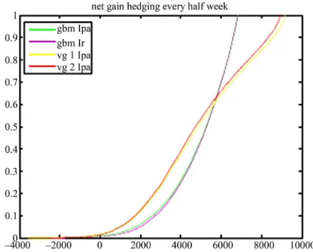
above. Figures 1 the gr empiric ula- ibution ns of t rofits

e methods above.

y comparing the numerical results we obtained so far, lowing conclusions:

The mean value of net gain from delta hedging every

n value of net gain from VG is larger than

DVG are close.

-3 show aph of al cum tive distr functio he net p through all th

6. Conclusions

B

we can make the fol



7 days is larger than hedging only once in the initial time.

 The mean value of net gain from delta hedging every 3 days is larger than hedging every 7 days.

 The mea

the mean from GBM.

 The mean value of net gain from GVG and

Figure 1. Empirical cdf of net profits of delta hedging once initially.

Figure 2. Empirical cdf of net profit of delta hedging every 7 days.

[image:4.595.56.287.401.506.2] [image:4.595.312.532.517.694.2]

(5)

L. Y. CAO ET AL. 124

7. References

[1] J. Hull, “Options, Futures, and Other Derivatives,” 5th Edition, Prentice Hall, Upper Saddle River, 2003.

[2] R. Jarrow and S. Turnbull, “Derivative Securities,” Thomson Learning Company, Belmont, 1999.

[3] M. C. Fu and J. Q. Hu, “Sensitivity Analysis for Monte Carlo Simulation of Option Pricing,” Engineering and Informational Sciences, Vol. 9, No. 3, 1995, pp. 417-446.

doi:10.1017/S0269964800003958

[4] P. Glasserman, “Monte Carlo Methods in Financial En-gineering,” Springer, New York, 2004.

[5] M. C. Fu, “What You Should Know about Simulation Derivatives,” Naval Research Logistics, Vol. 55, No. 8, 2006, pp. 723-736. doi:10.1002/nav.20313

and

nderson and B. L. Nelson, Eds., Handbooks in and Management Science, Elsevier, , pp. 575-616.

[6] M. C. Fu, “Stochastic Gradient Estimation,” In: S. G. He

tions Research sterdam, 2008

Am-[7] M. Broadie and P. Glasserman, “Estimating Security Price Derivatives Using Simulation,” Management Sci- ence, Vol. 42, No. 2, 1996, pp. 269-285.

doi:10.1287/mnsc.42.2.269

[8] F. Black and M. Scholes, “The Pricing of Options and Corporate Liabilities,” Journal of Political Economy, Vol. 81, No. 3, 1973, pp. 637-654. doi:10.1086/260062

[9] R. C. Merton, “Theory of Rational Option Pricing,” Jour- nal of Economics and Management Science, Vol. 4, No. 1, 1973, pp. 141-183.

[10] D. Madan and E. Seneta, “The Variance Gamma(VG) Model for Share Market Returns,” Journal of Business,

Vol. 63, No. 4, 1990, pp. 511-524. doi:10.1086/296519

[11] D. Madan and F. Milne, “Option Pricing with V.G. Mar-tingale Components,” Mathematical Finance, Vol. 1, 1991, pp. 39-55.

doi:10.1111/j.1467-9965.1991.tb00018.x

[12] D. Madan, P. Carr and E. Chang. “The Variance Gamma Processes and Option Pricing,” European Finance Re-view, Vol. 2, No. 1, 1998, pp. 79-10.

doi:10.1023/A:1009703431535

[13] M. C. Fu, “Variance-Gamma and Monte Carlo,” Advances in Mathematical Finance, Springer, 2007, pp. 21-35.

doi:10.1007/978-0-8176-4545-8_2

s for Variance [14] L. Cao and M. C. Fu, “Estimating Greek

Gamma,” Proceedings of the 2010 Winter Simulation Conference, Baltimore, 5-8 December 2010, pp. 2620- 2628. doi:10.1109/WSC.2010.5678958

ing Gradient Estimation

on-Nevada, 2-5 January

.

and Z. F. Guo, “Delta Hedging with Deltas from a [15] L. Cao and Z. F. Guo, “Apply

Technique to Estimate Gradients of European call fol-lowing Variance-Gamma,” Proceedings of Global C ference on Business and Finance,

2011.

[16] L. Cao and Z. F. Guo, “A Comparison of Gradient Esti-mation Techniques for European Call Options,” Ac-counting & Taxation, Forthcoming, 2011

[17] L. Cao and Z. F. Guo, “A Comparison of Delta Hedging under Two Price Distribution Assumptions by Likelihood Ratio,” International Journal of Business and Finance Research, Forthcoming, 2011.

[18] L. Cao