doi:10.4236/ajcm.2011.14031 Published Online December 2011 (http://www.SciRP.org/journal/ajcm)
Context-Dependent Data Envelopment Analysis with
Interval Data
Mohammad Izadikhah
Department of Mathematics, Islamic Azad University, Arak, Iran E-mail: [email protected], [email protected]
Received August 11, 2011; revised September 20, 2011; accepted September 28, 2011
Abstract
Data envelopment analysis (DEA) is a non-parametric method for evaluating the relative efficiency of deci-sion making units (DMUs) on the basis of multiple inputs and outputs. The context-dependent DEA is intro-duced to measure the relative attractiveness of a particular DMU when compared to others. In real-world situation, because of incomplete or non-obtainable information, the data (Input and Output) are often not so deterministic, therefore they usually are imprecise data such as interval data, hence the DEA models be-comes a nonlinear programming problem and is called imprecise DEA (IDEA). In this paper the con-text-dependent DEA models for DMUs with interval data is extended. First, we consider each DMU (which has interval data) as two DMUs (which have exact data) and then, by solving some DEA models, we can find intervals for attractiveness degree of those DMUs. Finally, some numerical experiment is used to illustrate the proposed approach at the end of paper.
Keywords:DEA, Context-Dependent, Interval Data, Interval Attractiveness, Interval Progress
1. Introduction
Data envelopment analysis (DEA), developed by Char-nes et al. [1], usually evaluates decision making units (DMUs) from the angle of the best possible relative effi-ciency. If a DMU is evaluated to have the best possible relative efficiency of unity, then it is said to be DEA ef-ficient; otherwise it is said to be DEA inefficient. Per-formance of inefficient DMUs depends on the efficient DMUs, that is, the inefficiency scores change only if the efficiency frontier is altered.
Although the performance of efficient DMUs is not influenced by the presence of inefficient DMUs, it is often influenced by the context. The context-dependent DEA [2-4] is introduced to measure the relative attrac-tiveness of a particular DMU when compared to others. We know that the DMUs in the reference set can be used as benchmark targets for inefficient DMUs. The con-text-dependent DEA provides several benchmark targets by setting evaluation context [3]. The context-dependent DEA is introduced to measure the relative attractiveness of a particular DMU when compared to others. Relative attractiveness depends on the evaluation context con-structed from alternative DMUs. The original DEA method evaluates each DMU against a set of efficient
DMUj is rated in the k-th place of ordinal variable and 0 otherwise. Extensions of these basic ideas are reported in [9,10]. Recently, Despotits and Smirlis [11] calculated upper and lower bounds for the efficiency scores of the DMUs with imprecise data. They developed an alterna-tion approach for dealing with imprecise data. They transformed the non-linear DEA model to a linear pro-gramming equivalent by using a straightforward formu-lation, completely different than that in IDEA. Contrarily to IDEA their transformation on the variables are made on the basis of the original data set, without applying any scale transformations on data. Also, in Jahanshahloo et al. [12,13] the radius of stability for the DMUs with interval data is calculated. In this paper we concentrate on the context-dependent DEA with interval data. For this rea-son we consider each DMUj, with interval data, as two DMUs that have exact data. Then by a procedure similar to that one in [3], the evaluation contexts are obtained by partitioning these DMUs into several levels of efficient frontier. Then by introducing some models based upon these efficient frontiers we can measure the relative at-tractiveness and progress of these DMUs and also we can determine the interval attractiveness and interval pro-gress for each original DMU with interval data. Further by combination of these measures we can also character-ize the performance of DMUs.
The rest of the paper is organized as follows: next sec-tion introduces the basic definisec-tions of interval data and notations of the original context-dependent DEA. In Sec-tion 3, interval context-dependent DEA is presented. In Section 4 we illustrate our proposed DEA method with two numerical examples and some discussion. Finally, some conclusions are pointed out in the end of this paper.
2. Preliminaries
Now suppose we have DMUs which utilize in-puts
n
m
, 1, ,
ij
x i m to produce s outputs
rj,
1, ,
,
1, ,
y r s
1 j n
, ,
. Also, assume that input and output levels of each DMU are not known exactly. We define Xj xj xmj and Yj
y1j,,ysj
,.
1, ,
j n
2.1. Interval Data
Let input and output values of any DMU be located in a certain interval, where xijL and
U ij
x are the lower and upper bounds of the i-th input of the DMUj, respecti- vely, and yrjL, are the lower and upper bounds of the r-th output of the
U rj
y
DMUj, respectively, that is to say,
L U
ij ij ij
x x x and yrLjyrjyUrj. Such data are called interval data, because they are located in intervals. Note that always xijLxUij and
L U
rj
y
rj
y . If xijL xijU, then
the i-th input of the DMUj has a definite value.
Interval problems are those whose parameter values are located in intervals, their exact values being unable to be identified.
Therefore we consider problems with data such as ,
L U ij ij ij
x x x and rj, rj L U
y
rj
y y , where lower and upper bounds are known exactly, positive and finite.
2.2. Context-Dependent Data Envelopment Analysis with Exact Data
The original context-dependent DEA model is developed by using the following radial efficiency measure. Let I1
be the set of all DMUs, and Ik and interactively defined as
k
E
1
k k k
I I E , where consists of all the radially efficient DMUs by following linear program-ming: k E
* 0 0 . . o o j jj j o
k
k k
s t X X
Y k
j F E ( ) ( ) max 0, k k
j F I
j F I
j
Y (1)where jF I
kmeans DMU k
jI
E
. When k = 1, model (1) becomes the original output oriented CCR model and define the first-level efficient frontier. When k = 2, model (1) gives the second-level efficient frontier after the exclusion of the first-level efficient DMUs. And so on. In this manner we identify several levels of efficient frontiers. We call the k-th level efficient frontier.
1
E
k
Assume that, , 0 . We can
calculate relative attractiveness measures for
with respect to k-th level efficient frontier. Based upon the evaluation context , relative attractiveness meas-ure of o can obtained by the following
con-text-dependent DEA:
0 k
k
E
DMUoE
k
E
0
1, ,
k n
DMUo DMU
0 0 ( ) ( ) ax 0, k k k k o o E E
0
*
0
0
0
m 1,...,
-. -.
j j j F
j j o
j F
k k j
H k H
X
k k L
s t X
Y H k Y
j F E k
(2)Then A ko*
1 Ho*
kDMUo 0, ,
k
k
is called the (output oriented) attractiveness of from a specific level Ek.
Model (2) is same as [3] with slightly change. In model (2) we set L 0 in order to consider-ing Ek0 as evaluation context for DMU k0.
oE
for DMUs with interval data.
3. Interval Context-Dependent DEA
Now, assume that there are n DMUs which produce s outputs yrj by using m inputs xij such that
, U
rj rj rj
y yL y and xij xijL,xUij. By considering each
DMUj as two DMUs with exact data, namely,
U
, L j j
X Y and
U, L
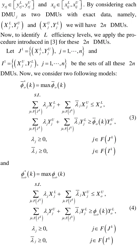
j jX Y we will have 2n DMUs. Now, to identify efficiency levels, we apply the pro-cedure introduced in [3] for these DMUs.
L
2n
Let 1
L, U
, 1, ,
j jJ X Y j n
Uj, jL , 1, ,and
1
I X Y j n be the sets of all these DMUs. Now, we consider two following models:
2n
* max . . , , 0, 0, k k k k o oL U L
j
j j j o
j F J j F I
U L
j o
j j j o
j F J j F I
k j
j
k k
s t
X X X
Y Y k
j F J
jF Ik
U Y (3) and
*max ( ) . . , , 0, 0, k k k k o o
L U U
j
j j j o
j F J j F I
U L
j L
j j j o
j F J j F I
k j
j
k k
s t
X X X
Y Y k
j F J
jF Ik o
Y (4)
Models (3) and (4) are similar to model (1) because these models simultaneously identify several levels of efficient frontiers as follows:
In the above models jF J
k means
L, U
j j k
X Y J and
k meansjF I
U, L
kj j
X Y I .
Then we define 1 1
k k k
J J E and 1 2
k k k
I I E , where 1
,
; *
k L U k
o j j
E X Y J k 1 and
*2 , ;
k U L k
j j o
E X Y I k 1
k
1
k
1
, then to identify k th-
level efficient DMUs, set 1 2 .
k k
E E E
When k = 1, then first-level efficient frontier is defined by DMUs in , that is, 2. When k = 2, models
(3) and (4) give the second-level efficient frontier after the exclusion the first-level efficient DMUs. In this manner we can identify several levels of efficient fron-tiers, where 1 2 consist the th-level efficient
frontier. By following steps we can identify these effi-cient frontiers using models (3) and (4):
1
E
E
1 1
E E
k
E
k
Step 1. Set k = 1, evaluate the DMUs belong to 1
J I using models (3) and (4) to obtain the first-level efficient DMUs, 1 2 .
k k
E E
Step 2. Set 1 1
k k k
J J E , 1 2
k k k
I I E . (If 1
k
J and k1
I then stop).
Step 3. Evaluate the new subset “inefficient” DMUs, 1
k
J , using models(3) and (4) to obtain new sets of effi-cient DMUs 1
1 k
E and . Set k = k + 1 and go to step 2.
1 2 k
E
[image:3.595.56.290.152.573.2]In the first section, we said that, the DMUs in the ref-erence set can be used as benchmark targets for ineffi-cient DMU. The context-dependent DEA provides sev-eral benchmark targets by setting evaluation context. DMUs can reach (if possible) to the nearest efficiency level as the first target to improve their efficiency.
Figure 1 plots the five levels of efficient frontiers of 5 DMUs with single interval input and single interval out-put (see Table 1). Assume that L levels of efficient fron-tiers are identified by the above algorithm. It can be seen that in this example L = 5.
Now based upon these evaluation contexts
, 1, , , k
E k L the context dependent DEA meas-ures the relative attractiveness of each DMU (DMUs with interval data) as follows:
Suppose for DMUo, by the above algorithm, we ob- tain
U, L
2o o l
X Y E and
L, U
l1o o
X Y E , clearly l1l2.
Output DMU2 DMU1 DMU3 DMU5 DMU4 E4 E5 E3 E2 E1 Input
[image:3.595.309.538.529.707.2]Table 1. Data of numerical example.
DMUj Inputs L j
x U
j
x Outputs L
j
y U
j
y
1 3.5 6 6 7
2 2.1 5 3 4.2
3 1.5 3 0.6 1.5
4 7.5 8 1.6 4.5
5 5 6 0.5 1
Now, we introduce two following context dependent DEA models to obtain the relative attractiveness meas-ure.
2 2 1 2 2 2 1 2 2 * 2 1max , 0, ,
. .
,
,
0,
0,
k l k l
k l k l
o o
L U L
j
j j j o
j F E j F E
U L
o j
j j j o
j F E j F E
k l j
j
H k H k k L l
s t
X X X
Y Y H
j F E
2
2 k l
jF E U k Y (5)
and
2 2 1 2 2 2 1 2 2 * 2 1max , 0, ,
. .
,
,
0,
0,
k l k l
k l k l
o o
L U U
j
j j j o
j F E j F E
U L
j o
j j j o
j F E j F E
k l j
j
H k H k k L l
s t
X X X
Y Y H
j F E
2
2
jF Ek l
L
k Y (6)
Clearly, H*o
k 1 and H*o
k 1 for 20, ,
k Ll , and also, *o
1
* o
H k H k and
* *
1
o o
H k H k .
Theorem 1. For DMUo we have Ho*
k Ho*
k ,2
Proof. First assume that
0, , .
k Ll
* *
, ,
o
H k * be optimal solution for model (5). Thus we have
2
2
1 2
k l k l
U L U L
o o
j
j j j o o
j F E j F E
Y Y H k Y H k Y
therefore
H*o
k , *,
*
is a feasible solution for
model (6). Since model (6) is maximization and has an optimal value as H*o
k , then
* *
o o
H k H k .
Corollary 1. If DMU
X Y, has exact data, whereL U
o o
X X X and YoL Y YoU, then we must have
* * *
2
, , 0, ,
o o
H k H k H k k L l
, where
*
H k
is the relative attractiveness measure for DMU. Assume that DMUo has interval data, that is,
U o , L
o o
X X X and Yo YoL,YoU. By Corollary 1,
*
*
*
2
, , 0, ,
o o .
H k H k H k k L l
Definition 1. If we call k-degree attractiveness of (which is lie on the specific level
DMUo
l2 l2 1
E E E2 2 l
) by A ko*
, then we have
* * * 1 1 , o o o A kH k H k
. That is, attractiveness score
of DMUo with respect to efficiency level Ek is
* o
A k .
Definition 2. We define
* *
1 1
,
o o
H k H k
as k-de-
gree attractiveness of DMUo.
Since the parameter values are located in intervals and their exact values being unable to be identified, hence value of A k*o
is unknown. Also, one can rank the DMUs in each level based upon their attractiveness scores.4. Application
In order to illustrate the use of the methodology for de-termining the interval attractiveness developed here, first, in example 1 we use the data in Table 1 and in example 2 we use an empirical data.
4.1. Example 1: Personal Selection Data
Assume that, we have 5 DMUs in one input and one output and these data are interval as shown in Table 1. By considering each DMUj as two DMUs with exact data, namely,
j, jU
L
X Y and
XUj,YjL
we will have 10 DMUs. Now, to identify the efficient levels of these DMUs, we apply models (3) and (4).Results are shown below:
1
1, 1 , 2, 2
L U L U
E X Y X Y
2
1 , 1 , 3, 3
U L L U
E X Y X Y
3
2, 2 , 4, 4
U L L U
E X Y X Y
4
3, 3 , 4, 4 , 5, 5
U L U L L U
E X Y X Y X Y
5
5, 5 U L
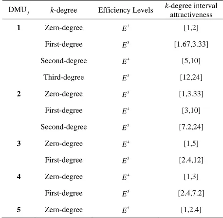
We see that for these DMUs, 5 efficient levels are identified, i.e., = 5. By models (5) and (6), interval attractiveness of each DMU can be calculated. In Table 2 interval attractiveness of each original DMUs (which have interval data) are shown in column 4. For example, in Table 2, first-degree interval attractiveness of
with respect to efficiency level is [1.67, 3.33].
L
1
DMU
3
E
That is, if we choose exact value for input and output of and then calculate the attractiveness degree of 1 with respect to efficiency level , namely
, we must have .
1
DMU DMU (3)
3
E
* 1
A 1.67A1*(3)3.33
Discussion
In the above mentioned example, suppose that, we fix the data of these DMUs in their intervals, in the other words, assume that we have 5 DMUs, namely,
DMUj X Yj, j , j1,,5, which have exact data
such that Xj XLj,XUj , Yj YjL,YjU. These data are as Table 3.
[image:5.595.308.537.349.518.2]We will show that, the attractiveness score of these DMUs lies in the interval attractiveness presented in Ta-
Table 2. Interval attractiveness.
DMUj k-degree Efficiency Levels
k-degree interval attractiveness
1 Zero-degree 2
E [1,2]
First-degree 3
E [1.67,3.33]
Second-degree 4
E [5,10]
Third-degree 5
E [12,24]
2 Zero-degree 3
E [1,3.33]
First-degree 4
E [3,10]
Second-degree 5
E [7.2,24]
3 Zero-degree 4
E [1,5]
First-degree 5
E [2.4,12]
4 Zero-degree 4
E [1,3]
First-degree 5
E [2.4,7.2]
5 Zero-degree 5
[image:5.595.56.285.367.591.2]E [1,2.4]
Table 3. DMUs with exact data.
DMUj Input Output
1 5 6
2 3 4
3 2 1
4 7.5 4.5
5 6 0.5
ble 2. Hence, we employ models (3) and (4) for these DMUs. Let Ek be the th-level of efficient frontier. See Figure 2 and compare
k
k
E and Ek. We define
kS E as follows:
1 1
, , , 0, ,
k
n n
k
j j j j j j j
j j
S E
x y x X y Y X Y E
For example, Figure 3 illustrates region of S E
k . It can be seen that,
5 5 4 4 3
3 2 2 1 1
S E S E S E S E S E
S E S E S E S E S E
Assume that, we want to calculate the attractiveness
degree of DMU1 with respect to efficiency level 4 E ,
that is, we want to calculate *
. Since 1 4A DMU1E2
and S E
3 S E
4 S E
4 , hence the attractivenessOutput
Input
DMU1
DMU2
DMU3
DMU5
DMU4 E1
E3
E4
E5
5 3
2
1
4
1
E 2
E E2
3
E
5
E
Figure 2. Levels of efficient froutiers for DMUs with exact data and interval data.
Output
Input
3
E
3S E
with respect to efficiency level E4, and 1
H*1
4
score of DMU1 lies in the following interval:and 1 H1*
3 are taken from Table 2.
1*
* *
1 1
1 1
4
4 A 3
H H Therefore, without direct calculation of attractiveness
scores of these DMUs (which have exact data) we must have
where A1*
4 is the attractiveness degree of DMU1
*
2 2 1,3.33 A
*
1 3 1.67,3.33
A *
2 3 1,3.33
A
*
1 4 1.67,10
A *
2 4 1,10
A *
4 4 1,3
A
*
1 5 12, 24
A *
2 5 7.2, 24
A *
3 5 2.4,12
A *
4 5 2.4,7.2
A
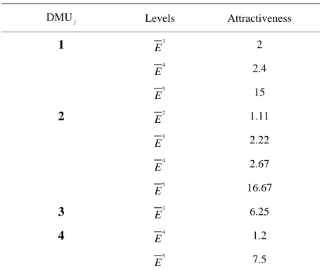
However, if we calculate attractiveness of this set of DMUs we have the Table 4 which shows that the above statement is true.
4.2. Example 2: Empirical Data
Consider a performance measurement problem of manu-facturing industry, in which there are eight manufactur-ing industries from different cities (DMUs) participatmanufactur-ing in the evaluation, each consuming two inputs (Labor and working funds) and producing three outputs (Gross in-dustrial output value, profit and taxes, and retail sales). The data are all estimated and are thus imprecise and only known within the prescribed bounds, which are listed in Table 5.
By using the DEA models (3) and (4) and by same manner as shown in example 1, we obtain the following levels of efficient frontiers:
1
1, 1 , 2, 2 , 7, 7 , 8, 8
L U L U L U L U
E X Y X Y X Y X Y
2
4, 4 , 5, 5
L U L U
E X Y X Y
3
1, 1 , 3, 3 , 6, 6 , 8, 8
L U L U L U L U
E X Y X Y X Y X Y
4
2, 2 , 3, 3 , 5, 5 , 7, 7
U L U L U L U L
E X Y X Y X Y X Y
5
4, 4 U L
E X Y
6
6, 6 U L
E X Y
Therefore, we see that for these DMUs, 6 efficient lev-els are identified, that is L6.
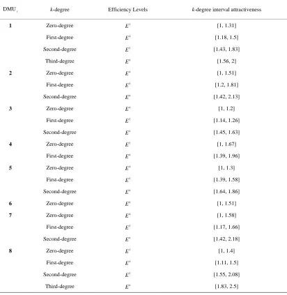
If we apply models (5) and (6) for these DMUs, we obtain interval attractiveness of each DMU as Table 6.
For instance, consider 1 which has interval data. By Table 6, one can see that interval attractiveness of 1 with respect to efficiency level is [1.18, 1.5]. Nevertheless, if one can find the exact value of and again calculate the attractiveness score of
1 with respect to , it must lie in interval [1.18, 1.5]. For more details see discussion presented in
exam-ple 1.
DMU
4
DMU
1
DMU DMU
4
E
E
Note: All the computations in this example are carried out by a computer program using GAMS software.
5. Conclusions
We developed in this paper an approach for dealing with interval data in context dependent DEA. It is done by considering each DMU (which have interval data) as two DMUs (which have exact data) and then we obtain in-terval attractiveness for each DMU. For this reason, we introduced some DEA models for evaluating these DMUs, and in the next step to obtain the interval attrac-tiveness we merge the results of these models. Also we show that, if we choose n arbitrary DMUs with exact data, then the attractiveness of these DMUs are belong to that intervals. After this manager decided that, what combination of each interval is appropriate.
2n
[image:6.595.309.538.520.713.2]Although the proposed method presented in this paper is illustrated by a personal selection data, however, it can also be applied to many problems of decision manage-
Table 4. Exact attractiveness for exact data of Table 3.
DMUj Levels Attractiveness
1 3
E 2
4
E 2.4
5
E 15
2 2
E 1.11
3
E 2.22
4
E 2.67
5
E 16.67
3 3
E 6.25
4 4
E 1.2
5
E 7.5
Table 5. Data for eight DMUs.
DMU Input Output
Labor Working Funds GIO Profit and Taxes Retail Sales
1 [66, 73] [1354, 1540] [3200, 3800] [1100, 1200] [1000,1150]
2 [54, 70] [1205, 1425] [3000, 3350] [1000, 1150] [800,930]
3 [65, 80] [950, 985] [2800, 3000] [800, 900] [650, 700]
4 [55, 63] [850, 1000] [2500, 2750] [800, 850] [600, 850]
5 [72, 85] [1105, 1200] [3050, 3700] [950, 1150] [1000, 1050]
6 [63, 80] [1250, 1380] [2700, 2900] [800, 950] [700, 750]
7 [57, 72] [950, 1150] [2950, 3250] [950, 1200] [800, 900]
[image:7.595.96.508.302.725.2]8 [60, 71] [800, 970] [2700, 2800] [800, 950] [900, 1000]
Table 6. Interval attractiveness of Example 2.
DMUj k-degree Efficiency Levels k-degree interval attractiveness
1 Zero-degree 3
E [1, 1.31]
First-degree 4
E [1.18, 1.5]
Second-degree 5
E [1.43, 1.83]
Third-degree 6
E [1.56, 2]
2 Zero-degree 4
E [1, 1.51]
First-degree 5
E [1.2, 1.81]
Second-degree 6
E [1.42, 2.13]
3 Zero-degree 4
E [1, 1.2]
First-degree 5
E [1.14, 1.26]
Second-degree 6
E [1.45, 1.63]
4 Zero-degree 5
E [1, 1.67]
First-degree 6
E [1.39, 1.96]
5 Zero-degree 4
E [1, 1.3]
First-degree 5
E [1.39, 1.58]
Second-degree 6
E [1.64, 1.86]
6 Zero-degree 6
E [1, 1.51]
7 Zero-degree 4
E [1, 1.58]
First-degree 5
E [1.17, 1.66]
Second-degree 6
E [1.42, 2.18]
8 Zero-degree 3
E [1, 1.4]
First-degree 4
E [1.11, 1.5]
Second-degree 5
E [1.55, 2.08]
Third-degree 6
ment. By the same manner one can use the proposed procedure to calculate interval progress for each DMU.
6. References
[1] A. Charnes, W. W. Cooper and E. Rhodes, “Measuring the Efficiency of Decision Making Units,” European Journal of Operational Research, Vol. 2, No. 6, 1978, pp. 429- 444. doi:10.1016/0377-2217(78)90138-8
[2] H. Morita, K. Hirokawa and J. Zhu, “A Slack-Based Mea- sure of Efficiency in Context Dependent Data Envelop- ment Analysis,” Omega, Vol. 33, No. 4, 2005, pp. 357- 362. doi:10.1016/j.omega.2004.06.001
[3] L. M. Seiford and J. Zhu, “Context-Dependent Data En- velopment Analysis: Measuring Attractiveness and Pro- gress,” Omega, Vol. 31, No. 5, 2003, pp. 397-408.
doi:10.1016/S0305-0483(03)00080-X
[4] J. Zhu, “Quantitative Models for Performance Evaluation and Benchmarking-Data Envelopment Analysis with Spread- sheets and DEA Excel Solver,” Kluwer, Boston, 2002. [5] W. W. Cooper, K. S. Park and G. Yu, “IDEA and AR-
IDEA: Models for Dealing with Imprecise Data in DEA,”
Management Science, Vol. 45, No. 4, 1999, pp. 597-607.
doi:10.1287/mnsc.45.4.597
[6] S. H. Kim, C. G. Park and K. S. Park, “An Application of Data Envelopment Analysis in Telephone Offices Evalu- ation with Partial Data,” Computers and Operations Re- search, Vol. 26, No. 1, 1999, pp. 59-72.
doi:10.1016/S0305-0548(98)00041-0
[7] W. D. Cook, M. Kress and L. Seiford, “Data Envelopment Analysis in the Presence of Both Quantitative and Quali- tative Factors,” Journal of the Operational Research So- ciety, Vol. 47, No. 7, 1996, pp. 945-953.
[8] W. D. Cook, M. Kress and L. Seiford, “On the Use of Ordinal Data in Data Envelopment Analysis,” Journal of the Operational Research Society, Vol. 44, No. 2, 1993, pp. 133-140.
[9] W. D. Cook, J. Doyle, R. Green and M. Kress, “Multiple Criteria Modeling and Ordinal Data: Evaluation in Terms of Subset of Criteria,” European Journal of Operational Research, Vol. 98, No. 3, 1997, pp. 602-609.
doi:10.1016/S0377-2217(96)00069-0
[10] J. Sarkis and S. Talluri, “A Decision Model for Evalua- tion of Flexible Manufacturing Systems in the Presence of Both Cardinal and Ordinal Factors,” International Journal of Production Research, Vol. 37, No. 13, 1999, pp. 2927-2938. doi:10.1080/002075499190356
[11] D. K. Despotis and Y. G. Smirlis, “Data Envelopment Ana- lysis with Imprecise Data,” European Journal of Opera-tional Research, Vol. 140, No. 1, 2002, pp. 24-36.
doi:10.1016/S0377-2217(01)00200-4
[12] G. R. Jahanshahloo, F. Hosseinzadeh Lotfi and M. Moradi, “Sensitivity and Stability Analysis in DEA with interval Data,” Applied Mathematics and Computation, Vol. 156, No. 2, 2004, pp. 463-477. doi:10.1016/j.amc.2003.08.005