Piecewise Latent Variables for Neural Variational Text Processing
Iulian V. Serban1∗and Alexander G. Ororbia II2∗and Joelle Pineau3 and Aaron Courville1 1Department of Computer Science and Operations Research, Universite de Montreal
2College of Information Sciences & Technology, Penn State University 3School of Computer Science, McGill University
iulian [DOT] vlad [DOT] serban [AT] umontreal [DOT] ca ago109 [AT] psu [DOT] edu
jpineau [AT] cs [DOT] mcgill [DOT] ca aaron [DOT] courville [AT] umontreal [DOT] ca
Abstract
Advances in neural variational inference have facilitated the learning of power-ful directed graphical models with con-tinuous latent variables, such as varia-tional autoencoders. The hope is that such models will learn to represent rich, multi-modal latent factors in real-world data, such as natural language text. How-ever, current models often assume simplis-tic priors on the latent variables — such as the uni-modal Gaussian distribution — which are incapable of representing com-plex latent factors efficiently. To over-come this restriction, we propose the sim-ple, but highly flexible, piecewise constant distribution. This distribution has the ca-pacity to represent an exponential num-ber of modes of a latent target distribution, while remaining mathematically tractable. Our results demonstrate that incorporating this new latent distribution into different models yields substantial improvements in natural language processing tasks such as document modeling and natural language generation for dialogue.
1 Introduction
The development of the variational autoencoder framework (Kingma and Welling,2014;Rezende et al.,2014) has paved the way for learning large-scale, directed latent variable models. This has led to significant progress in a diverse set of machine learning applications, ranging from computer vi-sion (Gregor et al.,2015; Larsen et al., 2016) to natural language processing tasks (Mnih and Gre-gor,2014;Miao et al.,2016;Bowman et al.,2015;
∗The first two authors contributed equally.
Serban et al.,2017b). It is hoped that this frame-work will enable the learning of generative pro-cesses of real-world data — including text, audio and images — by disentangling and representing the underlying latent factors in the data. How-ever, latent factors in real-world data are often highly complex. For example, topics in newswire text and responses in conversational dialogue of-ten posses laof-tent factors that follow non-linear (non-smooth), multi-modal distributions (i.e. dis-tributions with multiple local maxima).
Nevertheless, the majority of current models as-sume a simple prior in the form of a multivariate Gaussian distribution in order to maintain mathe-matical and computational tractability. This is of-ten a highly restrictive and unrealistic assumption to impose on the structure of the latent variables. First, it imposes a strong uni-modal structure on the latent variable space; latent variable samples from the generating model (prior distribution) all cluster around a single mean. Second, it forces the latent variables to follow a perfectly symmet-ric distribution with constant kurtosis; this makes it difficult to represent asymmetric or rarely occur-ring factors. Such constraints on the latent vari-ables increase pressure on the down-stream gen-erative model, which in turn is forced to carefully partition the probability mass for each latent factor throughout its intermediate layers. For complex, multi-modal distributions — such as the distribu-tion over topics in a text corpus, or natural lan-guage responses in a dialogue system — the uni-modal Gaussian prior inhibits the model’s ability to extract and represent important latent structure in the data. In order to learn more expressive latent variable models, we therefore need more flexible, yet tractable, priors.
prior distribution based on the piecewise constant distribution. We derive an analytical, tractable form that is applicable to the variational autoen-coder framework and propose a differentiable parametrization for it. We then evaluate the ef-fectiveness of the distribution when utilized both as a prior and as approximate posterior across variational architectures in two natural language processing tasks: document modeling and natu-ral language generation for dialogue. We show that the piecewise constant distribution is able to capture elements of a target distribution that can-not be captured by simpler priors — such as the uni-modal Gaussian. We demonstrate state-of-the-art results on three document modeling tasks, and show improvements on a dialogue natural lan-guage generation. Finally, we illustrate qualita-tively how the piecewise constant distribution rep-resents multi-modal latent structure in the data.
2 Related Work
The idea of using an artificial neural network to approximate an inference model dates back to the early work of Hinton and colleagues (Hinton and Zemel,1994;Hinton et al.,1995;Dayan and Hin-ton, 1996). Researchers later proposed Markov chain Monte Carlo methods (MCMC) (Neal, 1992), which do not scale well and mix slowly, as well as variational approaches which require a tractable, factored distribution to approximate the true posterior distribution (Jordan et al.,1999). Others have since proposed using feed-forward in-ference models to initialize the mean-field infer-ence algorithm for training Boltzmann architec-tures (Salakhutdinov and Larochelle,2010; Oror-bia II et al., 2015). Recently, the variational autoencoder framework (VAE) was proposed by Kingma and Welling (2014) and Rezende et al. (2014), closely related to the method proposed by Mnih and Gregor(2014). This framework allows the joint training of an inference network and a di-rected generative model, maximizing a variational lower-bound on the data log-likelihood and facil-itating exact sampling of the variational posterior. Our work extends this framework.
With respect to document modeling, neural ar-chitectures have been shown to outperform well-established topic models such as Latent Dirich-let Allocation (LDA) (Hofmann,1999;Blei et al., 2003). Researchers have successfully proposed several models involving discrete latent
vari-ables (Salakhutdinov and Hinton, 2009; Hinton and Salakhutdinov,2009;Srivastava et al.,2013; Larochelle and Lauly, 2012; Uria et al., 2014; Lauly et al.,2016;Bornschein and Bengio,2015; Mnih and Gregor,2014). The success of such dis-crete latent variable models — which are able to partition probability mass into separate regions — serves as one of our main motivations for investi-gating models with more flexible continuous latent variables for document modeling. More recently, Miao et al.(2016) proposed to use continuous la-tent variables for document modeling.
Researchers have also investigated latent vari-able models for dialogue modeling and dialogue natural language generation (Bangalore et al., 2008; Crook et al., 2009; Zhai and Williams, 2014). The success of discrete latent variable models in this task also motivates our investi-gation of more flexible continuous latent vari-ables. Closely related to our proposed ap-proach is the Variational Hierarchical Recur-rent Encoder-Decoder (VHRED, described below) (Serban et al.,2017b), a neural architecture with latent multivariate Gaussian variables.
Researchers have explored more flexible dis-tributions for the latent variables in VAEs, such as autoregressive distributions, hierarchical prob-abilistic models and approximations based on MCMC sampling (Rezende et al.,2014;Rezende and Mohamed, 2015; Kingma et al.,2016; Ran-ganath et al.,2016;Maaløe et al.,2016;Salimans et al.,2015;Burda et al.,2016;Chen et al.,2017; Ruiz et al.,2016). These are all complimentary to our approach; it is possible to combine them with the piecewise constant latent variables. In parallel to our work, multiple research groups have also proposed VAEs with discrete latent variables (Maddison et al., 2017; Jang et al.,2017; Rolfe, 2017;Johnson et al., 2016). This is a promising line of research, however these approaches often require approximations which may be inaccurate when applied to larger scale tasks, such as docu-ment modeling or natural language generation. Fi-nally, discrete latent variables may be inappropri-ate for certain natural language processing tasks.
3 Neural Variational Models
How-ever, the framework can easily be adapted to han-dle continuous output variables.
3.1 Neural Variational Learning
Let w1, . . . , wN be a sequence of N tokens
(words) conditioned on a continuous latent vari-able z. Further, letc be an additional observed variable which conditions bothzandw1, . . . , wN.
Then, the distribution over words is:
Pθ(w1, . . . , wN|c) =
� �N
n=1
Pθ(wn|w<n, z, c)Pθ(z|c)dz,
whereθare the model parameters. The model first generates the higher-level, continuous latent vari-ablezconditioned onc. Givenzandc, it then gen-erates the word sequencew1, . . . , wN. For
unsu-pervised modeling of documents, thecis excluded and the words are assumed to be independent of each other, when conditioned onz:
Pθ(w1, . . . , wN) =
� �N
n=1
Pθ(wn|z)Pθ(z)dz.
Model parameters can be learned using the varia-tional lower-bound (Kingma and Welling,2014):
logPθ(w1, . . . , wN|c)
≥ Ez∼Qψ(z|w1,...,wN,c)[logPθ(wn|w<n, z, c)]
−KL[Qψ(z|w1, . . . , wN, c)||Pθ(z|c)], (1)
where we note thatQψ(z|w1, . . . , wN, c) is the
approximation to the intractable, true posterior Pθ(z|w1, . . . , wN, c). Q is called the encoder,
or sometimes therecognition model orinference model, and it is parametrized byψ. The distri-bution Pθ(z|c) is the prior model for z, where
the only available information is c. The VAE framework further employs the re-parametrization trick, which allows one to move the derivative of the lower-bound inside the expectation. To ac-complish this,z is parametrized as a transforma-tion of a fixed, parameter-free random distribu-tion z = fθ(�), where � is drawn from a
ran-dom distribution. Here, f is a transformation of �, parametrized byθ, such thatfθ(�) ∼ Pθ(z|c).
For example, � might be drawn from a standard Gaussian distribution and f might be defined as fθ(�) =µ+σ�, whereµandσare in the
param-eter setθ. In this case,zis able to represent any Gaussian with meanµand varianceσ2.
Model parameters are learned by maximizing the variational lower-bound in eq. (1) using gra-dient descent, where the expectation is computed using samples from the approximate posterior.
The majority of work on VAEs propose to parametrize z as multivariate Gaussian distrib-tions. However, this unrealistic assumption may critically hurt the expressiveness of the latent vari-able model. See Appendix A for a detailed dis-cussion. This motivates the proposed piecewise constant latent variable distribution.
3.2 Piecewise Constant Distribution
We propose to learn latent variables by parametriz-ingzusing a piecewise constant probability den-sity function (PDF). This should allow z to rep-resent complex aspects of the data distribution in latent variable space, such as non-smooth regions of probability mass and multiple modes.
Letn∈Nbe the number of piecewise constant components. We assumezis drawn from PDF:
P(z) = K1 n
�
i=1
1�i−1
n ≤z≤ i n
�ai, (2)
where1(x)is the indicator function, which is one
whenxis true and otherwise zero. The distribu-tion parameters areai >0, fori= 1, . . . , n. The
normalization constant is:
K= n
�
i=1
Ki, whereK0= 0, Ki=ai
n, fori= 1, . . . , n.
It is straightforward to show that a piecewise con-stant distribution with more than n > 2 pieces is capable of representing a bi-modal distribution. When n > 2, a vector z of piecewise constant variables can represent a probability density with
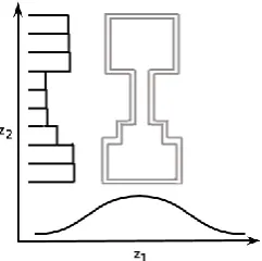
2|z|modes. Figure1illustrates how these variables help model complex, multi-modal distributions.
Figure 1: Joint density plot of a pair of Gaussian and piecewise constant variables. The horizontal axis corresponds toz1, which is a univariate
Gaus-sian variable. The vertical axis corresponds toz2,
which is a piecewise constant variable.
point is effectively zero. Thus, we fix these deriva-tives to zero. Similar approximations are used in training networks with rectified linear units.
4 Latent Variable Parametrizations In this section, we develop the parametrization of both the Gaussian variable and our proposed piecewise constant latent variable.
Letxbe the current output sequence, which the model must generate (e.g.w1, . . . , wN). Letcbe
the observed conditioning information. If the task contains additional conditioning information this will be embedded byc. For example, for dialogue natural language generation c represents an em-bedding of the dialogue history, while for docu-ment modelingc=∅.
4.1 Gaussian Parametrization
Letµpriorand σ2,prior be the prior mean and
vari-ance, and letµpostandσ2,postbe the approximate
posterior mean and variance. For Gaussian la-tent variables, the prior distribution mean and vari-ances are encoded using linear transformations of a hidden state. In particular, the prior distribu-tion covariance is encoded as a diagonal covari-ance matrix using a softplus function:
µprior=Hprior
µ Enc(c) +bpriorµ ,
σ2,prior=diag(log(1 + exp(Hprior
σ Enc(c) +bpriorσ ))),
where Enc(c)is an embedding of the conditioning informationc(e.g. for dialogue natural language generation this might, for example, be produced by an LSTM encoder applied to the dialogue his-tory), which is shared across all latent variable
dimensions. The matricesHµprior, Hσpriorand
vec-torsbpriorµ , bpriorσ are learnable parameters. For the
posterior distribution, previous work has shown it is better to parametrize the posterior distribution as a linear interpolation of the prior distribution mean and variance and a new estimate of the mean and variance based on the observationx(Fraccaro et al., 2016). The interpolation is controlled by a gating mechanism, allowing the model to turn on/off latent dimensions:
µpost=(1−α
µ)µprior+αµ�HµpostEnc(c, x) +bpostµ �,
σ2,post=(1−α
σ)σ2,prior
+ασdiag(log(1 + exp(HσpostEnc(c, x) +bpostσ ))),
where Enc(c, x) is an embedding of both c and x. The matrices Hµpost, Hσpost and the vectors bpostµ , bpostσ , αµ, ασ are parameters to be learned.
The interpolation mechanism is controlled byαµ
and ασ, which are initialized to zero (i.e.
initial-ized such that the posterior is equal to the prior).
4.2 Piecewise Constant Parametrization
We parametrize the piecewise prior parameters us-ing an exponential function applied to a linear transformation of the conditioning information:
apriori = exp(Ha,ipriorEnc(c) +bpriora,i ), i= 1, . . . , n,
where matrixHapriorand vectorbpriora are learnable.
As before, we define the posterior parameters as a function of bothcandx:
aposti = exp(Ha,ipostEnc(c, x) +bposta,i), i= 1, . . . , n,
whereHapostandbposta are parameters. 5 Variational Text Modeling
We now introduce two classes of VAEs. The mod-els are extended by incorporating the Gaussian and piecewise latent variable parametrizations.
5.1 Document Model
We refer to this model asP-NVDM. The second model we propose uses a combination of Gaus-sian and piecewise constant latent variables. The models sample the Gaussian and piecewise stant latent variables independently and then con-catenates them together into one vector. We refer to this model asH-NVDM.
Let V be the vocabulary of document words. LetWrepresent a document matrix, where rowwi
is the 1-of-|V|binary encoding of thei’th word in the document. Each model has an encoder com-ponent Enc(W), which compresses a document vector into a continuous distributed representa-tion upon which the approximate posterior is built. For document modeling, word order information is not taken into account and no additional condi-tioning information is available. Therefore, each model uses a bag-of-words encoder, defined as a multi-layer perceptron (MLP)Enc(c = ∅, x) =
Enc(x). Based on preliminary experiments, we choose the encoder to be a two-layered MLP with parametrized rectified linear activation functions (we omit these parameters for simplicity). For the approximate posterior, each model has the param-eter matrix Wapost and vector bposta for the
piece-wise latent variables, and the parameter matrices Wµpost, Wσpostand vectors bpostµ , bpostσ for the
Gaus-sian means and variances. For the prior, each model has parameter vector bpriora for the
piece-wise latent variables, and vectors bpriorµ , bpriorσ for
the Gaussian means and variances. We initialize the bias parameters to zero in order to start with centered Gaussian and piecewise constant priors. The encoder will adapt these priors as learning progresses, using the gating mechanism to turn on/off latent dimensions.
Letz be the vector of latent variables sampled according to the approximate posterior distribu-tion. Given z, the decoder Dec(w, z) outputs a distribution over words in the document:
Dec(w, z) = �exp (−wTRz+bw)
w�exp (−wTRz+bw�),
whereRis a parameter matrix andbis a parameter vector corresponding to the bias for each word to be learned. This output probability distribution is combined with the KL divergences to compute the lower-bound in eq. (1). See AppendixC.
Our baseline model G-NVDM is an improve-ment over the originalNVDMproposed byMnih and Gregor (2014) and Miao et al. (2016). We learn the prior mean and variance, while these
were fixed to a standard Gaussian in previous work. This increases the flexibility of the model and makes optimization easier. In addition, we use a gating mechanism for the approximate pos-terior of the Gaussian variables. This gating mech-anism allows the model to turn off latent vari-able (i.e. fix the approximate posterior to equal the prior for specific latent variables) when computing the final posterior parameters. Furthermore,Miao et al.(2016) alternated between optimizing the ap-proximate posterior parameters and the generative model parameters, while we optimize all parame-ters simultaneously.
5.2 Dialogue Model
The variational hierarchical recurrent encoder-decoder (VHRED) model has previously been pro-posed for dialogue modeling and natural language generation (Serban et al., 2017b, 2016a). The model decomposes dialogues using a two-level hi-erarchy: sequences of utterances (e.g. sentences), and sub-sequences of tokens (e.g. words). Letwn
be the n’th utterance in a dialogue withN utter-ances. Letwn,mbe them’th word in then’th
utter-ance from vocabularyV given as a 1-of-|V|binary encoding. LetMn be the number of words in the n’th utterance. For each utterancen = 1, . . . , N, the model generates a latent variablezn.
Condi-tioned on this latent variable, the model then gen-erates the next utterance:
Pθ(w1, z1, . . . ,wN, zN) = N
�
n=1
Pθ(zn|w<n)
× Mn �
m=1
Pθ(wn,m|wn,<m,w<n, zn),
whereθare the model parameters. VHRED con-sists of three RNN modules: an encoder RNN, a context RNN and a decoder RNN. The en-coderRNN computes an embedding for each ut-terance. This embedding is fed into the context
RNN, which computes a hidden state summariz-ing the dialogue context before utterancen:hcon
n−1.
This state represents the additional conditioning information, which is used to compute the prior distribution overzn:
Pθ(zn|w<n) =fθprior(zn;hconn−1),
wherefprioris a PDF parametrized by bothθand hcon
to thedecoderRNN, which then computes the out-put probabilities of the words in the next utterance. The model is trained by maximizing the varia-tional lower-bound, which factorizes into indepen-dent terms for each sub-sequence (utterance):
logPθ(w1, . . . ,wN)
≥�N n=1
−KL[Qψ(zn |w1, . . . ,wn)||Pθ(zn|w<n)]
+EQψ(zn|w1,...,wn)[logPθ(wn|zn,w<n)],
where distributionQψis the approximate posterior
distribution with parameters ψ, computed simi-larly as the prior distribution but further condi-tioned on the encoder RNN hidden state of the next utterance.
The original VHRED model (Serban et al., 2017b) used Gaussian latent variables. We re-fer to this model as G-VHRED. The first model we propose uses piecewise constant latent vari-ables instead of Gaussian latent varivari-ables. We re-fer to this model asP-VHRED. The second model we propose takes advantage of the representation power of both Gaussian and piecewise constant la-tent variables. This model samples both a Gaus-sian latent variable zgaussiann and a piecewise
la-tent variable znpiecewise independently conditioned
on thecontextRNN hidden state:
Pθ(zngaussian|w<n) =fθprior, gaussian(zngaussian;hconn−1), Pθ(zpiecewisen |w<n) =fθprior, piecewise(zpiecewisen ;hconn−1),
where fprior, gaussian and fprior, piecewise are PDFs
parametrized by independent subsets of parame-tersθ. We refer to this model asH-VHRED.
6 Experiments
We evaluate the proposed models on two types of natural language processing tasks: document modeling and dialogue natural language genera-tion. All models are trained with back-propagation using the variational lower-bound on the log-likelihood or the exact log-log-likelihood. We use the first-order gradient descent optimizer Adam (Kingma and Ba, 2015) with gradient clipping (Pascanu et al.,2012)1
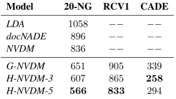
Model 20-NG RCV1 CADE
LDA 1058 −− −−
docNADE 896 −− −−
NVDM 836 −− −−
G-NVDM 651 905 339
H-NVDM-3 607 865 258
[image:6.595.319.501.83.185.2]H-NVDM-5 566 833 294
Table 1: Test perplexities on three document mod-eling tasks: 20-NewGroup (20-NG), Reuters cor-pus (RCV1) and CADE12 (CADE). Perplexities were calculated using 10 samples to estimate the variational lower-bound. The H-NVDM models perform best across all three datasets.
6.1 Document Modeling
Tasks We use three different datasets for docu-ment modeling experidocu-ments. First, we use the 20 News-Groups (20-NG) dataset (Hinton and Salakhutdinov,2009). Second, we use the Reuters corpus (RCV1-V2), using a version that con-tained a selected 5,000 term vocabulary. As in previous work (Hinton and Salakhutdinov, 2009;Larochelle and Lauly,2012), we transform the original word frequencies using the equation
log(1 +TF), where TF is the original word fre-quency. Third, to test our document models on text from a non-English language, we use the Brazilian Portuguese CADE12 dataset (Cardoso-Cachopo, 2007). For all datasets, we track the validation bound on a subset of 100 vectors randomly drawn from each training corpus.
Training All models were trained using mini-batches with 100 examples each. A learning rate of0.002was used. Model selection and early stop-ping were conducted using the validation lower-bound, estimated using five stochastic samples per validation example. Inference networks used 100 units in each hidden layer for 20-NG and CADE, and 100 for RCV1. We experimented with both
50and100latent random variables for each class of models, and found that50latent variables per-formed best on the validation set. ForH-NVDM
we vary the number of components used in the PDF, investigating the effect that 3 and 5 pieces had on the final quality of the model. The number
1Code and scripts are available athttps://github.
com/ago109/piecewise-nvdm-emnlp-2017
and https://github.com/julianser/
G-NVDM H-NVDM-3 H-NVDM-5
environment project science project gov built
flight major high
lab based technology
mission earth world launch include form field science scale
working nasa sun
[image:7.595.92.284.82.226.2]build systems special gov technical area
Table 2: Word query similarity test on 20 News-Groups: for the query ‘space”, we retrieve the top 10 nearest words in word embedding space based on Euclidean distance. H-NVDM-5 asso-ciates multiple meanings to the query, while G-NVDMonly associates the most frequent meaning.
of hidden units was chosen via preliminary exper-imentation with smaller models. On 20-NG, we use the same set-up as (Hinton and Salakhutdi-nov,2009) and therefore report the perplexities of a topic model (LDA, (Hinton and Salakhutdinov, 2009)), the document neural auto-regressive esti-mator (docNADE, (Larochelle and Lauly,2012)), and a neural variational document model with a fixed standard Gaussian prior (NVDM, lowest re-ported perplexity, (Miao et al.,2016)).
Results In Table 1, we report the test docu-ment perplexity:exp(−1
D
�
nL1n logPθ(xn). We
use the variational lower-bound as an approxima-tion based on 10 samples, as was done in (Mnih and Gregor, 2014). First, we note that the best baseline model (i.e. theNVDM) is more competi-tive when both the prior and posterior models are learnt together (i.e. theG-NVDM), as opposed to the fixed prior of (Miao et al., 2016). Next, we observe that integrating our proposed piecewise variables yields even better results in our docu-ment modeling experidocu-ments, substantially improv-ing over the baselines. More importantly, in the 20-NG and Reuters datasets, increasing the num-ber of pieces from 3 to 5 further reduces perplex-ity. Thus, we have achieved a new state-of-the-art perplexity on 20 News-Groups task and — to the best of our knowledge – better perplexities on the CADE12 and RCV1 tasks compared to us-ing a state-of-the-art model like theG-NVDM. We also evaluated the converged models using an non-parametric inference procedure, where a separate
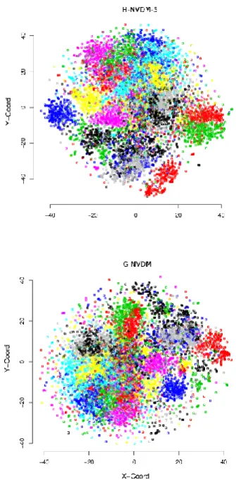
Figure 2: Latent variable approximate poste-rior means t-SNE visualization on 20-NG for G-NVDMandH-NVDM-5. Colors correspond to the topic labels assigned to each document.
approximate posterior is learned for each test ex-ample in order to tighten the variational lower-bound.H-NVDMalso performed best in this eval-uation across all three datasets, which confirms that the performance improvement is due to the piecewise components. See appendix for details.
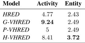
[image:7.595.316.484.87.428.2]Model Activity Entity
HRED 4.77 2.43
G-VHRED 9.24 2.49
P-VHRED 5 2.49
[image:8.595.119.258.84.155.2]H-VHRED 8.41 3.72
Table 3: Ubuntu evaluation using F1 metrics w.r.t. activities and entities. G-VHRED,P-VHREDand
H-VHRED all outperform the baseline HRED.
G-VHRED performs best w.r.t. activities and H-VHREDperforms best w.r.t. entities.
the word. More examples are in the appendix. Finally, we visualized the means of the approx-imate posterior latent variables on 20-NG through a t-SNE projection. As shown in Figure2, both
G-NVDM and H-NVDM-5 learn representations which disentangle the topic clusters on 20-NG. However, G-NVDM appears to have more dis-persed clusters and more outliers (i.e. data points in the periphery) compared to H-NVDM-5. Al-though it is difficult to draw conclusions based on these plots, these findings could potentially be ex-plained by the Gaussian latent variables fitting the latent factors poorly.
6.2 Dialogue Modeling
TaskWe evaluateVHREDon a natural language generation task, where the goal is to generate re-sponses in a dialogue. This is a difficult prob-lem, which has been extensively studied in the recent literature (Ritter et al., 2011; Lowe et al., 2015; Sordoni et al., 2015; Li et al., 2016; Ser-ban et al.,2016a,b). Dialogue response generation has recently gained a significant amount of atten-tion from industry, with high-profile projects such as Google SmartReply (Kannan et al.,2016) and Microsoft Xiaoice (Markoff and Mozur, 2015). Even more recently, Amazon has announced the Alexa Prize Challenge for the research community with the goal of developing a natural and engaging chatbot system (Farber,2016).
We evaluate on the technical support response generation task for the Ubuntu operating system. We use the well-known Ubuntu Dialogue Corpus (Lowe et al.,2015,2017), which consists of about 1/2 million natural language dialogues extracted from the #Ubuntu Internet Relayed Chat (IRC) channel. The technical problems discussed span a wide range of software-related and hardware-related issues. Given a dialogue history — such
as a conversation between a user and a technical support assistant — the model must generate the next appropriate response in the dialogue. For ex-ample, when it is the turn of the technical support assistant, the model must generate an appropriate response helping the user resolve their problem.
We evaluate the models using the activity- and entity-based metrics designed specifically for the Ubuntu domain (Serban et al., 2017a). These metrics compare theactivitiesand entities in the model generated responses with those of the ref-erence responses; activities are verbs referring to high-level actions (e.g. download, install, unzip) and entities are nouns referring to technical ob-jects (e.g.Firefox, GNOME). The more activities and entities a model response overlaps with the reference response (e.g. expert response) the more likely the response will lead to a solution.
Training The models were trained to maxi-mize the log-likelihood of training examples us-ing a learnus-ing rate of 0.0002 and mini-batches of size 80. We use a variant of truncated back-propagation. We terminate the training procedure for each model using early stopping, estimated using one stochastic sample per validation exam-ple. We evaluate the models by generating dia-logue responses: conditioned on a diadia-logue con-text, we fix the model latent variables to their me-dian values and then generate the response using a beam search with size 5. We select model hyper-parameters based on the validation set using the F1 activity metric, as described earlier.
It is often difficult to train generative models for language with stochastic latent variables (Bow-man et al., 2015; Serban et al.,2017b). For the latent variable models, we therefore experiment with reweighing the KL divergence terms in the variational lower-bound with values 0.25, 0.50,
0.75 and1.0. In addition to this, we linearly in-crease the KL divergence weights starting from zero to their final value over the first75000 train-ing batches. Finally, we weaken thedecoderRNN by randomly replacing words inputted to the de-coder RNN with the unknown token with 25%
probability. These steps are important for effec-tively training the models, and the latter two have been used in previous work by Bowman et al. (2015) andSerban et al.(2017b).
HRED (Baseline): We compare to theHRED
es-tablished models on this task, such as the LSTM RNN language model (Serban et al.,2017a). The
HREDmodel’sencoderRNN uses a bidirectional GRU RNN encoder, where the forward and back-ward RNNs each have 1000 hidden units. The context RNN is a GRU encoder with1000hidden units, and the decoder RNN is an LSTM decoder with 2000 hidden units.2 The encoder and
con-text RNNs both use layer normalization (Ba et al., 2016).3 We also experiment with an additional
rectified linear layer applied on the inputs to the decoder RNN. As with other hyper-parameters, we choose whether to include this additional layer based on the validation set performance. HRED, as well as all other models, use a word embedding dimensionality of size400.
G-HRED: We compare toG-VHRED, which isVHREDwith Gaussian latent variables (Serban et al., 2017b). G-VHREDuses the same hyper-parameters for the encoder, context and decoder RNNs as the HRED model. The model has 100
Gaussian latent variables per utterance.
P-HRED: The first model we propose is P-VHRED, which isVHREDmodel with piecewise constant latent variables. We usen = 3number of pieces for each latent variable. P-VHREDalso uses the same hyper parameters for the encoder, context and decoder RNNs as theHRED model. Similar to G-VHRED, P-VHRED has100 piece-wise constant latent variables per utterance.
H-HRED: The second model we propose is H-VHRED, which has100piecewise constant (with n = 3pieces per variable) and100Gaussian la-tent variables per utterance. H-VHREDalso uses the same hyper-parameters for the encoder, con-text and decoder RNNs asHRED.
Results: The results are given in Table 3. All latent variable models outperformHREDw.r.t. both activities and entities. This strongly suggests that the high-level concepts represented by the latent variables help generate meaningful, goal-directed responses. Furthermore, each type of latent variable appears to help with a different aspects of the generation task. G-VHRED per-forms best w.r.t. activities (e.g.download, install
and so on), which occur frequently in the dataset.
2Since training lasted between 1-3 weeks for each model,
we had to fix the number of hidden units during preliminary experiments on the training and validation datasets.
3We did not apply layer normalization to the decoder
RNN, because several of our colleagues have found that this may hurt the performance of generative language models.
This suggests that the Gaussian latent variables learn useful latent representations for frequent ac-tions. On the other hand, H-VHRED performs best w.r.t. entities (e.g. Firefox,GNOME), which are often much rarer and mutually exclusive in the dataset. This suggests that the combination of Gaussian and piecewise latent variables help learn useful representations for entities, which could not be learned by Gaussian latent variables alone. We further conducted a qualitative analysis of the model responses, which supports these conclu-sions. See AppendixG.4
7 Conclusions
In this paper, we have sought to learn rich and flexible multi-modal representations of latent vari-ables for complex natural language processing tasks. We have proposed the piecewise constant distribution for the variational autoencoder frame-work. We have derived closed-form expressions for the necessary quantities required for in the au-toencoder framework, and proposed an efficient, differentiable implementation of it. We have in-corporated the proposed piecewise constant dis-tribution into two model classes — NVDM and
VHRED— and evaluated the proposed models on document modeling and dialogue modeling tasks. We have achieved state-of-the-art results on three document modeling tasks, and have demonstrated substantial improvements on a dialogue modeling task. Overall, the results highlight the benefits of incorporating the flexible, multi-modal piece-wise constant distribution into variational autoen-coders. Future work should explore other natural language processing tasks, where the data is likely to arise from complex, multi-modal latent factors. Acknowledgments
The authors acknowledge NSERC, Canada Re-search Chairs, CIFAR, IBM ReRe-search, Nuance Foundation and Microsoft Maluuba for fund-ing. Alexander G. Ororbia II was funded by a NACME-Sloan scholarship. The authors thank Hugo Larochelle for sharing the News-Group 20 dataset. The authors thank Lau-rent Charlin, Sungjin Ahn, and Ryan Lowe for constructive feedback. This research was en-abled in part by support provided by Calcul Qubec (www.calculquebec.ca) and Com-pute Canada (www.computecanada.ca).
References
J. L. Ba, J. R. Kiros, and G. E. Hinton. 2016. Layer normalization.arXiv preprint arXiv:1607.06450. S. Bangalore, G. Di Fabbrizio, and A. Stent. 2008.
Learning the structure of task-driven human–human dialogs. IEEE Transactions on Audio, Speech, and Language Processing, 16(7):1249–1259.
D. M. Blei, A. Y. Ng, and M. I. Jordan. 2003. Latent dirichlet allocation. JAIR, 3:993–1022.
J. Bornschein and Y. Bengio. 2015. Reweighted wake-sleep. InICLR.
S. R. Bowman, L. Vilnis, O. Vinyals, A. M. Dai, R. Jozefowicz, and S. Bengio. 2015. Generating sentences from a continuous space. InConference on Computational Natural Language Learning. Y. Burda, R. Grosse, and R. Salakhutdinov. 2016.
Im-portance weighted autoencoders.ICLR.
A. Cardoso-Cachopo. 2007. Improving Methods for Single-label Text Categorization. PdD Thesis, Insti-tuto Superior Tecnico, Universidade Tecnica de Lis-boa.
X. Chen, D. P. Kingma, T. Salimans, Y. Duan, P. Dhari-wal, J. Schulman, I. Sutskever, and P. Abbeel. 2017. Variational lossy autoencoder. InICLR.
N. Crook, R. Granell, and S. Pulman. 2009. Unsuper-vised classification of dialogue acts using a dirichlet process mixture model. In Special Interest Group on Discourse and Dialogue (SIGDIAL), pages 341– 348.
P. Dayan and G. E. Hinton. 1996. Varieties of helmholtz machine. Neural Networks, 9(8):1385– 1403.
L. Devroye. 1986. Sample-based non-uniform random variate generation. InProceedings of the 18th con-ference on Winter simulation, pages 260–265. ACM.
M. Farber. 2016. Amazon’s ’Alexa Prize’ Will Give College Students Up To $2.5M To Create A Social-bot. Fortune.
M. Fraccaro, S. K. Sønderby, U. Paquet, and O. Winther. 2016. Sequential neural models with stochastic layers. InNIPS, pages 2199–2207. K. Gregor, I. Danihelka, A. Graves, and D. Wierstra.
2015. DRAW: A recurrent neural network for image generation. InICLR.
G. E. Hinton, P. Dayan, B. J. Frey, and R. M. Neal. 1995. The” wake-sleep” algorithm for unsupervised neural networks.Science, 268(5214):1158–1161. G. E. Hinton and R. Salakhutdinov. 2009. Replicated
softmax: an undirected topic model. InNIPS, pages 1607–1614.
G. E. Hinton and R. S. Zemel. 1994. Autoencoders, minimum description length and helmholtz free en-ergy. InNIPS, pages 3–10. NIPS.
T. Hofmann. 1999. Probabilistic latent semantic index-ing. In ACM SIGIR Conference on Research and Development in Information Retrieval, pages 50–57. ACM.
E. Jang, S. Gu, and B. Poole. 2017. Categorical repa-rameterization with gumbel-softmax. InICLR.
M. Johnson, D. K. Duvenaud, A. Wiltschko, R. P. Adams, and S. R. Datta. 2016. Composing graphical models with neural networks for structured repre-sentations and fast inference. InNIPS, pages 2946– 2954.
M. I. Jordan, Z. Ghahramani, T. S. Jaakkola, and L. K. Saul. 1999. An introduction to variational methods for graphical models. Machine Learning, 37(2):183–233.
A. Kannan, K. Kurach, et al. 2016. Smart Reply: Au-tomated Response Suggestion for Email. InKDD.
D. Kingma and J. Ba. 2015. Adam: A method for stochastic optimization. InICLR.
D. P. Kingma, T. Salimans, and M. Welling. 2016. Im-proving variational inference with inverse autore-gressive flow. NIPS, pages 4736–4744.
D. P. Kingma and M. Welling. 2014. Auto-encoding variational Bayes. ICLR.
H. Larochelle and S. Lauly. 2012. A neural autoregres-sive topic model. InNIPS, pages 2708–2716.
A. B. Lindbo Larsen, S. K. Sønderby, and O. Winther. 2016. Autoencoding beyond pixels using a learned similarity metric. InICML, pages 1558–1566.
S. Lauly, Y. Zheng, A. Allauzen, and H. Larochelle. 2016. Document neural autoregressive distribution estimation. arXiv preprint arXiv:1603.05962.
J. Li, M. Galley, C. Brockett, J. Gao, and B. Dolan. 2016. A diversity-promoting objective function for neural conversation models. InThe North American Chapter of the Association for Computational Lin-guistics (NAACL), pages 110–119.
Ryan Lowe, Nissan Pow, Iulian Serban, and Joelle Pineau. 2015. The Ubuntu Dialogue Corpus: A Large Dataset for Research in Unstructured Multi-Turn Dialogue Systems. InSpecial Interest Group on Discourse and Dialogue (SIGDIAL).
Lars Maaløe, Casper Kaae Sønderby, Søren Kaae Sønderby, and Ole Winther. 2016. Auxiliary deep generative models. InICML, pages 1445–1453. C. J. Maddison, A. Mnih, and Y. W. Teh. 2017. The
concrete distribution: A continuous relaxation of discrete random variables. InICLR.
J. Markoff and P. Mozur. 2015. For Sympathetic Ear, More Chinese Turn to Smartphone Program. New York Times.
Y. Miao, L. Yu, and P. Blunsom. 2016. Neural varia-tional inference for text processing. InICML, pages 1727–1736.
A. Mnih and K. Gregor. 2014. Neural variational in-ference and learning in belief networks. InICML, pages 1791–1799.
R. M. Neal. 1992. Connectionist learning of belief net-works.Artificial intelligence, 56(1):71–113. A. G. Ororbia II, C. L. Giles, and D. Reitter. 2015.
Online semi-supervised learning with deep hybrid boltzmann machines and denoising autoencoders. arXiv preprint arXiv:1511.06964.
R. Pascanu, T. Mikolov, and Y. Bengio. 2012. On the difficulty of training recurrent neural networks. ICML, 28:1310–1318.
Rajesh Ranganath, Dustin Tran, and David Blei. 2016. Hierarchical variational models. In ICML, pages 324–333.
D. J. Rezende and S. Mohamed. 2015. Variational in-ference with normalizing flows. In ICML, pages 1530–1538.
D. J. Rezende, S. Mohamed, and D. Wierstra. 2014. Stochastic backpropagation and approximate infer-ence in deep generative models. In ICML, pages 1278–1286.
A. Ritter, C. Cherry, and W. B. Dolan. 2011. Data-driven response generation in social media. In Pro-ceedings of the Conference on Empirical Methods in Natural Language Processing, pages 583–593. J. T. Rolfe. 2017. Discrete variational autoencoders. In
ICLR.
Francisco R Ruiz, Michalis Titsias RC AUEB, and David Blei. 2016. The generalized reparameteriza-tion gradient. InNIPS, pages 460–468.
R. Salakhutdinov and G. E. Hinton. 2009. Semantic hashing. International Journal of Approximate Rea-soning, 50(7):969–978.
R. Salakhutdinov and H. Larochelle. 2010. Efficient learning of deep boltzmann machines. InAISTATs, pages 693–700.
T. Salimans, D. P Kingma, and M. Welling. 2015. Markov chain monte carlo and variational inference: Bridging the gap. InICML, pages 1218–1226.
R. Sennrich, B. Haddow, and A. Birch. 2016. Neu-ral machine translation of rare words with subword units. InAssociation for Computational Linguistics (ACL).
I. V. Serban, T. Klinger, G. Tesauro, K. Talamadupula, B. Zhou, Y. Bengio, and A. Courville. 2017a. Mul-tiresolution recurrent neural networks: An applica-tion to dialogue response generaapplica-tion. InThirty-First AAAI Conference (AAAI).
I. V. Serban, A. Sordoni, Y. Bengio, A. Courville, and J. Pineau. 2016a. Building end-to-end dialogue sys-tems using generative hierarchical neural network models. InThirtieth AAAI Conference (AAAI). I. V. Serban, A. Sordoni, R. Lowe, L. Charlin,
J. Pineau, A. Courville, and Y. Bengio. 2017b. A hierarchical latent variable encoder-decoder model for generating dialogues. InThirty-First AAAI Con-ference (AAAI).
Iulian Vlad Serban, Ryan Lowe, Laurent Charlin, and Joelle Pineau. 2016b. Generative deep neural net-works for dialogue: A short review. InNIPS, Let’s Discuss: Learning Methods for Dialogue Workshop. A. Sordoni, M. Galley, M. Auli, C. Brockett, Y. Ji, M. Mitchell, J. Nie, J. Gao, and B. Dolan. 2015. A neural network approach to context-sensitive gen-eration of conversational responses. InConference of the North American Chapter of the Association for Computational Linguistics (NAACL-HLT 2015), pages 196–205.
N. Srivastava, R. R Salakhutdinov, and G. E. Hin-ton. 2013. Modeling documents with deep boltz-mann machines. InProceedings of the Twenty-Ninth Conference on Uncertainty in Artificial Intelligence (UAI), pages 616–624.
B. Uria, I. Murray, and H. Larochelle. 2014. A deep and tractable density estimator. In ICML, pages 467–475.