Abstract— We propose a new modified algorithm for the Branch and Bound method. This method is based on integration of orthogonal arrays and enumeration based techniques. Several observations are given supplemented with simple model solutions to verify our assumptions. The modified algorithm is valid for higher dimensional problems. The algorithm employs several 2-levels orthogonal arrays and the
complexity of solutions is always of the order2n . For low to medium size problems, full factorial orthogonal arrays are employed. For higher size problems, the user uses fractional orthogonal arrays and the complexity of solution is always of
the order 2n−k, k≤n. Results show that full size arrays yield optimum solution consistently. When fractional arrays are used, the solution is always incumbent. The number of function evaluations is always low. We show that this conclusion, though true, is rare as the number of continuous solutions resulting from relaxations is always tractable with full size arrays. This method utilizes the fact that the number of continuous solutions from relaxations is lesser than the original problem size. Numerical results show that the proposed hybrid algorithm is able to save 20% ~ 96% of the original computations. Fractional arrays allow fractionation and consequent deviation from the best solution.
Index Terms— Approximation, B. & B. Algorithms,
optimization, hybrid techniques.
I. INTRODUCTION
Standard optimization methods such as Branch and Bound (B. & B.) are used to deal with problems that are 0-1 binary programming, mixed integer programming (MIP) and general integer programming (IP). B. & B. method is efficient but size dependent. Engineering problem synthesis, analysis and improvements are becoming crucial nowadays. As knowledge advances, problem analysis and synthesis increase in complexity. Accordingly, the synthesis tool should develop at the same pace.
Manuscript received April 18, 2009. Mohamed H. Gadallah is Associate Professor, Department of Operations Research, Institute of Statistical Studies & Research, Cairo University, Cairo, Egypt 12613 (phone: 202-37484624; fax: 202-37482533; e-mail: [email protected]).
Most realistic problems are complex to solve with existing optimization techniques. We admit that there are complex realistic engineering problems, commonly known as NP-hard. This hardship is due to the problem size, combinatorial nature, storage capacity, etc. Part of hardship, of course, is due to the synthesis phase “how to model the optimization problem?” An algorithm is developed that integrates the B. & B. method with orthogonal arrays and enumeration techniques. The search domain is modeled using orthogonal arrays (full or fractional) and enumeration techniques. We show that there is equivalence between both the space used and the resulting problem solution. The proposed algorithm can determine the search size and accordingly the cost of solution. For the first time, the algorithm gives the user the flexibility to choose the solution quality and corresponding cost. In case a high quality solution is required, the modeller should be ready to compromise time and effort. Several situations do not require quality solutions; accordingly, the user can resort to fractional arrays to model the problem. Integration of B. and B. algorithm, orthogonal arrays and enumeration techniques is novel to our knowledge and the engineering community should welcome such means of hybridization as long as they offer solution to hard to solve problems.
Realistic engineering applications are size dependent. The engineering community is either considering the option of over simplification of the original problem or resort to hybrid methods. Over simplification yields trivial solutions. The B.& B. algorithm is the search engine, the orthogonal arrays are the search domains and enumeration techniques are the possibilities of all model formulations. Due to space limitation, past studies are not included.
II. NOMENCLATURE
n
2 2 levels factorial design, n=# of variables.
OA 4
L 4 experiments, 2-levels orthogonal arrays.
ij
X Decision variables from i to j.
f Objective function.
c
X Continuous form of decision variable X.
OA 64
L 64 experiments, 2-levels orthogonal arrays. 64
P , , 1
P … 64 sub-models.
min
f Minimum objective value. max
f Maximum objective value. 11
P A diverse of sub-model P1
Computer Simulation-based Optimization:
Hybrid Branch & Bound and Orthogonal Array
based Enumeration Algorithm
ij
Y Decision variables from i to j.
OA 2
L 2-levels orthogonal array (single variable). 121
P A diverse of sub-model P12 122
P Another diverse of sub-model P12 o
P Original model (after relaxation). OA
16
L 16 experiments, 2-levels orthogonal arrays.
OA 32
L 32 experiments, 2-levels orthogonal arrays. 1
k k
2 Fractional factorial, 2 levels arrays (K ≥ K1).
*
X Optimum solution of decision variable. OA
536 , 65
L 65,536 exp., 2-levels orthogonal arrays.
OA 2048
L 2048 experiments, 2-levels orthogonal arrays.
OA
∞
L Very huge, 2-levels orthogonal arrays (244).
III. METHODOLOGY
Table 1 shows the array sizes used for different number of variables. The full and fractional arrays are given with the probability of finding the best solution (optimum). For instance, an L4OA is used to model 2 variables with a probability of 100% to find the optimum. As the number of variables increase to 3, the array size changes from L4OA to L8OA. The analyst has an option of using : a) an L8OA and 100% probability of getting the best solution or b) an L4OA and 50% probability of getting the best solution. Equivalently, L16OA is used to model 4 variables with a probability of 100% to find the best solution. Similarly, the analyst may decide to fractionate by using L8OA (and L4OA). In this case, the probability of finding the best solution is 50% for L8OA. As the number of variables increase to 9, the array size becomes L512OA (for the full
array), L256OA (for half of the array), L128OA (for the quarter of array), L64OA (for the 1/8 of array) and L32OA (for the 1/16 of array) respectively. When the user uses the full size array, the probability of getting the best solution is 100%. Once he decides to fractionate, the probability of getting the best solution is equivalent to the fraction value. For instance, when L256OA is used to model a 9-variable problem, the probability becomes 25%. Ideally the modeller will try to employ the full size arrays to enjoy the best solutions. Full size arrays are tractable, easy to code and understand for low size problems (n ≤ 5~6 variables). For a medium size problem with
n
≥
15
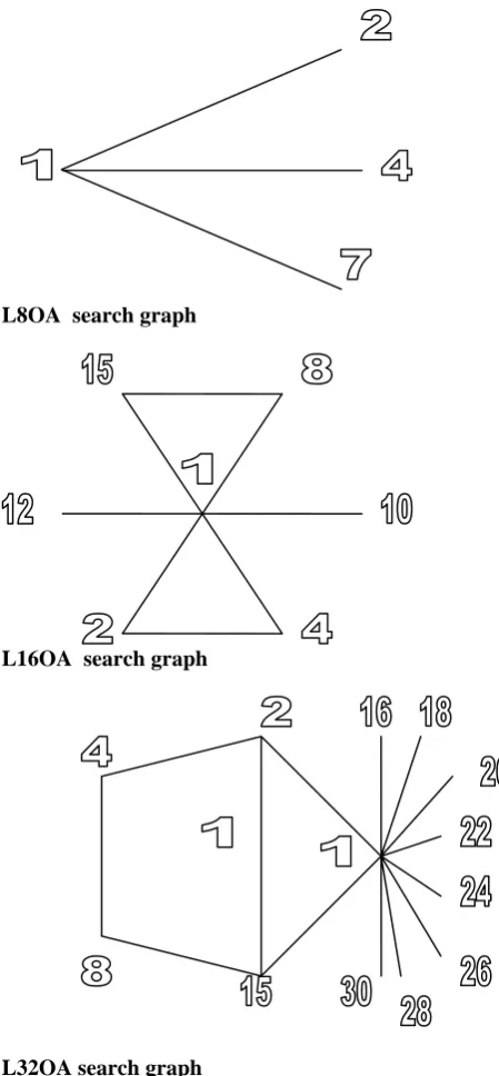
variables, the size becomes 215 = 32,768and only then, the modeller will start to realize the benefit of fractionation. [image:2.595.79.522.490.672.2]Different search graphs assign continuous variables resulting from constraint relaxation to different arrays columns. Figure 1 gives different search graphs for L8OA, L16OA and L32OA respectively. For instance, when L8OA is used, variables can be assigned to columns 1, 2 and 4 (for a full array) or 1, 2, 4 and 7 (for a half array). Similarly, when L16OA is used, variables can be assigned to columns 1, 2, 4 and 8 (for a full array) or 1,2,4,8 and 15 (for a half array) or 1,2,4,8,15 and 12 (for a quarter array) respectively. Similar assignments can be followed once L32OA is used.
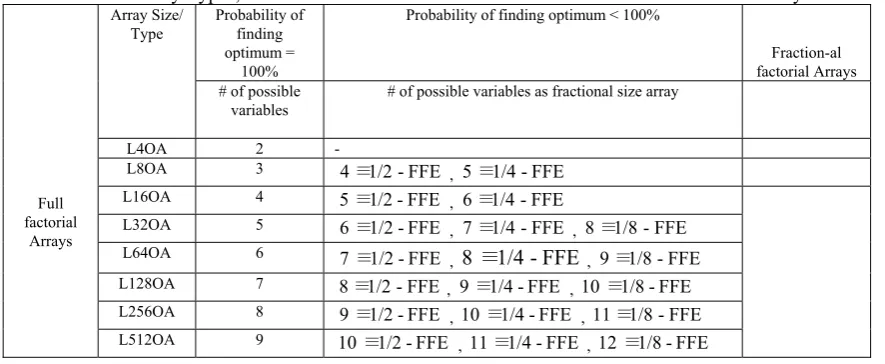
Table 1: Array Types, Maximum Number of Modeled Variables for Full & Fractional Arrays.
Probability of finding optimum =
100%
Probability of finding optimum < 100%
Fraction-al factorial Arrays Array Size/
Type
# of possible variables
# of possible variables as fractional size array
L4OA 2 -
L8OA 3 4≡1/2 -FFE , 5≡1/4 -FFE
L16OA 4 5≡1/2-FFE , 6≡1/4-FFE
L32OA 5 6≡1/2-FFE , 7≡1/4-FFE, 8≡1/8-FFE
L64OA 6 7≡1/2-FFE , 8≡1/4-FFE, 9≡1/8-FFE
L128OA 7 8≡1/2-FFE, 9≡1/4-FFE , 10≡1/8-FFE
L256OA 8 9≡1/2-FFE , 10≡1/4-FFE , 11≡1/8-FFE
Full factorial
Arrays
L8OA search graph
L16OA search graph
[image:3.595.46.271.46.531.2]L32OA search graph
Fig. 1: L8OA, L16OA and L32OA and corresponding search graphs.
Case Study 1: MIMCK Problem [5].
This is a model with 21 continuous and 9 binary 0,1 variables and linear objective and 4 inequality constraints. The model is given as:
Maximize 33 Y 5 32 Y 3 31 Y 4 23 Y 6 22 Y 7 21 Y 13 Y 3 12 Y 6 11 Y 3 37 X 9 36 X 5 35 X 3 34 X 8 33 X 4 32 X 4 31 X 2 27 X 7 26 X 6 25 X 3 24 X 6 23 X 4 22 X 6 21 X 2 17 X 7 16 X 6 15 X 5 14 X 6 13 X 8 12 X 5 11 X 3 f + + + + + + + + + + + + + + + + + + + + + + + + + + + + + = s.t.: 1 g : 40 ≤ 33 Y 32 Y 6 31 Y 7 23 Y 4 22 Y 6 21 Y 2 13 Y 4 12 Y 5 11 Y 7 37 X 3 36 X 35 X 6 34 X 2 33 X 4 32 X 2 31 X 5 27 X 3 26 X 5 25 X 6 24 X 3 23 X 22 X 2 21 X 5 17 X 4 16 X 5 15 X 6 14 X 3 13 X 4 12 X 2 11 X + + + + + + + + + + + + + + + + + + + + + + + + + + + + + 2
g : 1
17 X 16 X 15 X 14 X 13 X 12 X 11 X ≤ + + + + + + ; 3
g : ≤ 1
27 X 26 X 25 X 24 X 23 X 22 X 21 X + + + + + + ; 4
g : ≤ 1
37 X 36 X 35 X 34 X 33 X 32 X 31 X + + + + + + ; 5
g : Xki ≥ 0, k=1,2,3, i=1,2, ,7 6
g : Ykj∈{0,1}, k=1,2,3, j=1,2,3
When the model is synthesized as continuous, the best maximum reached is $56.50.
) 1 , 0 , 0 , 0 , 0 , 0 , 0 , 1 , 0 , 0 , 0 , 0 , 0 , 0 , 0 , 0 , 0 , 0 , 1 , 0 , 0 ( c
X = and
) 1 , 5 . 0 , 1 , 1 , 1 , 0 , 1 , 1 , 0 ( c
Y = and fmax =56.50. Two sub-models are formulated and shown in Table 2.
Table 2: Different Sub-models, corresponding Y conditions and fmaxvalues.
Prob 32
Y fmax Solution
111
P :Y11 ≤ 0,
max
f =56, optimum
11
P ≤ 0 56.43 0.14
11
Y =
112
P :Y11 ≥ 1,
max
f =55.71
121
P :Y31 ≤ 0,
max
f =55.86
12
P ≥ 1 56.29 0.57
31
Y =
122
P :Y31 ≥ 1,
max
f =55.75
The 2 sub-models are given below: 11
P : Maximize f Subject to: g1, g4 ; 1 ≤ 33 Y 12 Y , 11 Y ≤
0 … ; Y32 ≤ 0
11
111
P : Maximize f Subject to: g1 , g4 ; 1 ≤ 33 Y 12 Y , 11 Y ≤
0 … ; Y32 ≤ 0, Y11 ≤ 0 111
P yields fmax=56 and this is the optimum value. 112
P : Maximize f Subject to: g1 , g4 ; 1 ≤ 33 Y 12 Y , 11 Y ≤
0 … ; Y32 ≤ 0, Y11 ≥ 1 112
P yields fmax=55.71. 12
P : Maximize f Subject to: g1, g4 1 ≤ 33 Y 12 Y , 11 Y ≤
0 … ; Y32 ≥ 1
12
P yields fmax =56.29 and Y31 = 0.57 . P12 will produce 2 further sub-models: P121 & P122
121
P : Maximize f Subject to: g1 , g4 ; 1 ≤ 33 Y 12 Y , 11 Y ≤
0 … ; Y32 ≥ 1, Y31 ≤ 0 121
P yields fmax =55.86. 122
P : Maximize f Subject to: g1 , g4 ; 1 ≤ 33 Y 12 Y , 11 Y ≤
0 … ; Y32 ≥ 1, Y31 ≥ 1
122
P yields fmax =55.75.
Case Study 2: Limitations to Fractional Based Search We present a case study with 30 binary integer program. We show how the fractional search fails to obtain the best solution because of problem size. This model is known as Maximum Coverage EMS Model [17] and is given by: Minimize 20 Y 9 . 9 19 Y 9 . 7 18 Y 3 . 5 17 Y 11 16 Y 6 . 25 15 Y 5 . 15 14 Y 3 . 9 13 Y 12 12 Y 9 . 30 11 Y 4 . 30 10 Y 3 . 20 9 Y 6 . 7 8 Y 2 . 12 7 Y 10 6 Y 7 . 5 5 Y 1 . 6 4 Y 0 . 9 3 Y 1 . 7 2 Y 4 . 4 1 Y 2 . 5 f + + + + + + + + + + + + + + + + + + + =
s.t.: g1: X2 +Y1≥ 1 g2 : X1+X2 +Y2≥ 1 ; 3
g : X1+X3+Y3 ≥ 1 ;g4 :X3+Y4 ≥ 1 ; 5
g :X3+Y5≥1 ;g6 :X2 +Y6 ≥ 1 ; 7
g :X2 +X4 +Y7 ≥ 1 ;g8: X3+X4 +Y8≥ 1 ; 9
g : X8+Y9 ≥ 1 ;g10: X4+X6+Y10 ≥ 1 ; 11
g :X4+X5+Y11≥ 1 ; 12
g :X4+X5+X6+Y12 ≥ 1 ; 13
g : X4+X5+X7 +Y13 ≥ 1 ; 14
g : X8+X9 +Y14 ≥ 1 ; 15
g : X6+X9+Y15 ≥ 1 ; 16
g : X5+X6+Y16 ≥ 1 ; 17
g : X5+X7 +X10+Y17 ≥ 1 ; 18
g : X8+X9+Y18 ≥ 1 ;g19: 1 ≥ 19 Y 10 X 9
X + + ;
20
g : X10+Y20 ≥ 1 ;g21: 4 j X 10 1 j ≤ ∑
= ;Y1 Y20 0,1 1 , 0 10 X 1 X = =
Relaxation of P0 model yields
5 . 0 20 Y 9 Y 6 Y 5 Y 4 Y 3 Y 2 Y 1
Y = = = = = = = = and
5 . 0 10 X 9 X 8 X 6 X 5 X 4 X 3 X 2
X = = = = = = = = This
means that the continuous branching variables = 16 (out of 30 original variable). The array size becomes
OA 536 , 65 L ⇔ 536 , 65 = 16
2 . Certainly this is very
prohibitive array size. The full size array is very hard to develop and the assignment of variables to L65,536OA is cumbersome. This means that full size arrays, search graphs, quality and cost of solution are very restrictive. Fractional arrays and corresponding approximate solutions are considered. Accordingly, an L32OA is used to model the 16 branching variables. We could not use L16OA as it has 15 degrees of freedom (can host only 15 variables). This model is made of 30 variables and 21 constraints. Constraints are of equality/ inequality nature. Pure enumeration method yields a hard-to-solve problem. With the L32OA, 32 sub-models are formulated and solutions are recorded. Only 5 solution results and 27 models returned “a no-feasible solution”. The solutions are summarized in Table 3 for brevity. For instance, Trial # 14 has Y2 =Y3 =Y20 =X2 =2, (2nd level, =1) and
1 = 4 X = 6
Y , (1st level, = 0). In other words, six further
variables can be fixed and the 16 variable relaxed model becomes 10 instead of 16. Further insight reveals no function value difference between Trial 14 and 32. Hence, setting Y1,Y4,Y5,X5,X8,X9at 1st level or 2nd level
has no impact on the objective function. The same can be stated for Y9,X3,X6,X10respectively. Another look at trials # 4 and # 25 would conclude that different variable settings would result in almost similar function values
3 . 67
fmin = for trial # 4 vs. fmin = 68.7 for trial # 25. Y3,Y4,X6,X9 can be set at the 1st level and
5 X , 3 X , 9 Y , 6
Y can be set at the high level. This means the 16 variable model can be reduced to an 8 variable model. Besides, Y1,Y2,X8,X10set at either the low or high levels would not affect the objective function. A similar conclusion can be stated for Y5,Y20,X2,X4 respectively. Four sets of experiments are given next. Experiment 1: Effect of Y1,Y2 on solution
2 Y , 1
Y are modelled using L4OA. 4 sub-models are formulated and solved. All sub-models yielded “no-feasible solution”.
Experiment 2: Effect of Y1,Y2,Y3,Y4on solution
4 Y , 3
Y are modelled using L4OA with Y1,Y2≤ 0 . 4 sub-models are formulated and solved. All sub-models yielded “no-feasible solution”.
Experiment 3: Effect of Y1,Y2,Y3,Y4,Y5,Y6 on solution
6 Y , 5
Y are modelled using L4OA with
. 0 ≤ 4 Y , 3 Y , 0 ≤ 2 Y , 1
Table 3: Maximum Coverage Problem using L32OA
Trial 1
Y Y2 Y3 Y4 Y5 Y6 Y9 Y20 X2 X3 X4 X5 X6 X8 X9 X10 fmin
4 1 1 1 1 2 2 2 2 2 2 2 2 1 1 1 1 fmin =67.3
8 1 1 2 2 2 2 2 2 2 2 1 1 1 1 2 2 fmin =152.6
14 1 2 2 1 1 1 2 2 2 2 1 1 2 1 1 2 fmin=74
25 2 2 1 1 1 2 2 1 1 2 1 2 1 2 1 2 =68.7
min f
32 2 2 2 2 2 1 1 2 2 1 1 2 1 2 2 1 74.2
min
f =
0 ≤
≡
1 , 2≡≥1
Experiment 4: Effect of 20 Y , 9 Y , 6 Y , 5 Y , 4 Y , 3 Y , 2 Y , 1
Y on solution
20 Y , 9
Y are modelled using L4OA with
. 0 ≤ 20 Y , 9 Y , 0 ≤ 4 Y , 3 Y , 0 ≤ 2 Y , 1
Y 4 sub-models are
formulated and solved. All sub-models yielded “no-feasible solution”.
With these preliminary results, we can assert that L32OA is not enough to model the problem and other larger size array has to be used. Besides, we can conclude that the model has no feasible solution with
. 0 ≤ 20 Y , 9 Y , 6 Y , 5 Y , 4 Y , 3 Y , 2 Y , 1 Y
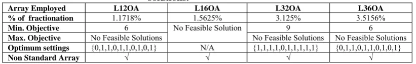
[image:5.595.93.504.501.565.2]Case Study 3: Minimum Coverage Problem [17]. This is a problem with 10 binary 0,1 variables and linear objective and constraints. The model is given as:
Table 4: Different Fractional Arrays & model solutions.
Minimize ∑Xj 10
1 j f
= =
s.t.: g1:X2≥ 1; g2 :X1+X2 ≥ 1; 3
g :X1+X3≥ 1;g4 : X3≥ 1; g5: X2≥ 1; 6
g : X2+X4 ≥ 1;g7 : X3+X4 ≥ 1;g8: 1
≥ 2
X ;g9: X6 +X4 ≥ 1; g10 : 1
≥ 5 X 4
X + ;g11: X4+X5+X6≥ 1;g12 : 1
≥ 7 X 5 X 4
X + + ; g13:X8 +X9 ≥ 1;g14 : 1
≥ 9 X 6
X + ;g15: X6 +X5 ≥ 1;g16 : 1
≥ 5 X 4
X + ;g17: X7 +X5+X10 ≥ 1;g18: 1
≥
9 X + 8
X ;g19 : X10 +X9 ≥ 1;g20 : 1
≥ 10
X ; Xij =0,1;
The model is synthesized as 0-1. The best minimum reached is 6. Four idealizations are given in Table 4 using
, OA 16 L , OA 12
L L32OA,L36OA respectively.
Array Employed L12OA L16OA L32OA L36OA
% of fractionation 1.1718% 1.5625% 3.125% 3.5156%
Min. Objective 6 9 6
Max. Objective No Feasible Solutions
No Feasible Solution
No Feasible Solutions No Feasible Solutions
Optimum settings {0,1,1,0,1,1,0,1,0,1} N/A {1,1,1,1,0,1,1,1,1,1} {0,1,1,0,1,1,0,1,0,1}
Non Standard Array √ √ √ √
IV RESULTS & DISCUSSION
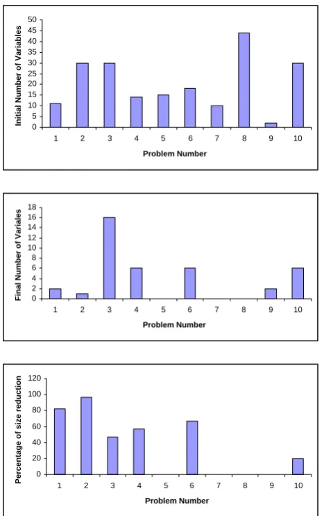
Table 5 gives a summary of all problems examined. The original model is described in terms of # of variables, # of constraints, nature of problems and solution obtained. The maximum number of continuous variables is also given. The maximum number of continuous variables is 16 (out of 30) for the Max_MCEMS_1. This is the only exception out of the problems tested. In the reduced model, the sizes of different arrays used to model the resulting space range from L2OA ~ L64OA. The employed orthogonal array sizes are 2-levels arrays of acceptable sizes and the cost is
always 2n. The cost of the method employed is always affordable. Compared with the regular B. and B.
0 5 10 15 20 25 30 35 40 45 50
1 2 3 4 5 6 7 8 9 10
Problem Number
In
itia
l Nu
mb
e
r o
f Va
ri
a
b
le
s
0 2 4 6 8 10 12 14 16 18
1 2 3 4 5 6 7 8 9 10
Problem Number
Fi
na
l N
u
mbe
r of
Va
ri
a
le
s
0 20 40 60 80 100 120
1 2 3 4 5 6 7 8 9 10
Problem Number
P
ercentage of si
z
e reducti
[image:6.595.47.281.49.421.2]on
[image:6.595.323.555.51.465.2]Fig. 2: Summary of test cases.
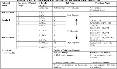
Table 6 gives description of different arrays. Only 2-level arrays are used, some are standard such as L4OA, L8OA, L16OA, L32OA and L64OA. Others are not standard such as L128OA, L256OA, L512OA, L1024OA and L2048OA. The development of search graphs for non standard arrays and high number of variables is a novel area of research. This research only utilizes existing search graphs for standard low size arrays. The knowledge of search graphs limits the use of non standard arrays, although can be used. These standard and non standard arrays can model 1~11 variables (for standard arrays) and 3~15 (for non standard arrays). Low size arrays are less expensive than large size arrays. The full size arrays require expensive # of function evaluations and CPU time. The results obtained are high quality unique solutions. When fractional arrays are used, certainly more variables can be modelled at the expense of non-unique solutions. The solution expense increases with the number of variables and size of array. The algorithm developed is given in figure 3.
Start
Input Model with obj. fn., constraints, DV
Is DV 0,1
Yes
No 1
Construct 2^n Array
Obj. fn and Constraint fn.
calculation
Check feasibility
Best Feasible solution
Exit
1 2
2
Is DV continuous,
Integer ?
Activate relaxation tech.
Solve LP, Po How many Continuous Var.
3
Yes Establish Different Models
Solve Respective
Models
Enumerate To obtain best solution for Maximization
Exit Construct Half
Array (1/2 FFE) Construct Full
Array (FFE)
4
Random Assignment
of Var. 3
Fig. 3: B. & B. Algorithm via Orthogonal Array Based Enumeration Techniques
V. CONCLUSIONS
• NP-hard problems can be solved via the proposed method in a cost effective manner.
• The method proved applicable to LP problems. Extension to quadratic and nonlinear problems requires linearization techniques about a point.
• Orthogonal arrays used, so far, are 2k of acceptable size. Further larger size problems need to check the solution expense of arrays employed.
• The proposed method needs a comparative analysis with other methods vs. the size of different problems. This will help place our method relative to others with respect to problem nature, size, complexity, applicability and objective/ constraint types.
Table 5: Description of Different Models Tested. ♣ Standard OAs. ♠ Non-standard OAs. #-o-V: # of Variables, #-o-C: # of Constraints, N-o-C: Nature of Constraints, Ineq = Inequality, Eq = Equality Constraints, Pr-N: Problem Nature
Size of Array Used Original Model B. & B.
Algorithm
Reduced Model
Problem #-o-V #-o-C N-o-C Solution Pr- N # of Continuous
Variables # of Sub-models
Before relaxation
After relaxation
% of Size reduction
SSWFC_1 [17] 11 17 Best MIP 2 L4OA L2048♠ L4 OA♣ 81.8%
MIMCK_1[5] 30 6 Best MIP 1 L2OA L1,073
E+09
L2 OA 96.6%
Max_MCEMS_1 [17]
30 21 Ineq
Best 0-1 16 L65,536 L1,073
E +09
L65,536 OA
♠
46.67%
NASA_1[17] 14 13 Good
Enough
0-1 6 No
relaxations L16,384♠ L64 OA♣
57.14%
AACS_1[17] 15 12
Eq
Best 0-1 0 - L32,768 - -
CDOT_1[17] 18 9 Eq/
Ineq
Best 0-1 6 L64 OA –
L32 OA - L16OA
L262,144♠ L64 OA♣ 66.67%
Min_MCEMS_1 [17]
10 20 Ineq Best 0-1 0 - L1024 - -
Cam- Assignment_1 [17]
44 20 Eq Best 0-1 0 - L∞♠ - -
Mitch_1[13] 2 2 Ineq Best General
Integer 2 L4OA L4OA L4OA♣
0.0%
Waste_1[17] 30 24 Eq/
Ineq
Best MIP 6 L64 OA –
L32 OA L16OA L8OA
L∞ L64OA♣ 20%
Table 6: Illustrative description of different arrays used & their relative cost.
2-Levels Arrays
Full Array Fractional Array Nature of
Array
Knowledge of Search Graph
Array Size # of variables Type of Array # of variables (Fractional Array)
Non-standard √ L2OA 1
√ L4OA 2 3
√ L8OA 3 4
√ L16OA 4 5,6 (1/2, ¼)
√ L32OA 5 6,7,8,9 (1/2, ¼, 1/8, 1/16)
Standard
√ L64OA 6 7,8,9,10,11
(1/2, ¼, 1/8, 1/16, 1/32)
× L128OA 7 8, 9, 10, 11, 12
(1/2, ¼, 1/8, 1/16, 1/32)
× L256OA 8 9, 10, 11, 12, 13, 14
(1/2, ¼, 1/8, 1/16, 1/32, 1/64)
× L512OA 9 11, 12, 13, 14, 15
× L1024OA 10 12, 13, 14, 15 (1/2, ¼, 1/8,
1/16)
Non-standard
× L2048OA 11
Low Expense
Full Factorial
High Expense
Quality of Solutions Obtained
Full Size Arrays Fractional Size Arrays
1. High quality solution. 1. Low to moderate quality solution
2. Unique (best solution). 2. Non-unique solution.
√: available
×: not available
3. May be expensive for larger size problems.
[image:7.595.66.529.404.678.2]REFERENCES
[1] Bin, Yu and Baozong, Yuan “A More Efficient Branch and Bound Algorithm for Feature Selection”, Pattern Recognition, Vol. 26, n6, 1993, pp. 883-889.
[2] Boris Goldengorin, Diptesh Ghosh, Gerard Sier Ksma, “Branch and Peg Algorithms for The Simple Plant Location Problem”,
Computers and Operations Research, Vol. 31, 2004, pp. 241-255. [3] Chao-Y Gau, Linus E. Schrage “Implementation and Testing of a
Branch and Bound Based Method for Deterministic Global Optimization: Operations Research Applications”, Frontiers In Global Optimization, C.A. Floudas and P.M. Pardalos, Editors, 2003, Kluwer Academic Publishers, pp. 1-20.
[4] Ghaith Rabadi , Mansoreeh Mollaghasemi, Georgios C. Anognostoploulous “A Branch and Bound Algorithm for the Early/ Tardy Machine Scheduling Problem with a Common Due Date and Sequence Dependent Setup Time”, J. of Computers & Operation Research, 2003, pp. 1-25.
[5] George Kozanidis and Emanuel Melachrionoudis “ A Branch & Bound Algorithm for the 0-1 Mixed Integer Knapsack Problem with Linear Multiple Choice Constraints”, Computers & Operations Research, Vol. 31, 2004, pp. 695-711.
[6] Gadallah, M.H., Ameer Al-Salem, Khalifa Al-Khalifa, Tamer A. Mohamed, “A Modified Branch & Bound Algorithm via Orthogonal Array Based Enumeration Techniques – Background Method & Preliminary Results”, 7th World Congress on Structural and
Multidisciplinary Optimization, Coex Seoul, Korea, 2007. [7] James, R.J.W and Storer, R.H. “Techniques for Solving Subset Sum
Problems Within a given Tolerance”, International Transactions in Operational Research, Vol. 12, 4, 2005, pp. 437-453.
[8] Kent Andersen, Gerard Cornuejols, Yanjun, Li “Reduce and Split Cuts: Improving the Performance of Mixed Integer Gomory Cuts”,
Management Science, Vol. 51 no. 11, 2005, pp. 1720-1732.
[9] Klincewicz, J.G. “Enumeration and Search Procedure for a Hub Location Problem with Economies of Scale”, Annals of Operations Research, Vol. 110, 2002, pp. 107-122.
[10] Klincewicz, J.G. “Enumeration and Search Procedure for a Hub Location Problem with Economies of Scale”, Annals of Operations Research, Vol. 110, 2002, pp. 107-122.
[11] Lieshout, P.M.D and Volgenant, A. “A Branch and Bound Algorithm for the Singly Constrained Assignment Problem”,
European Journal of Operational Research, Vol. 176, n1, 2007,
pp. 151-164.
[12] Liming Cai, Juedes D. , Kanji, I. “The In-approximability of Non-Hard Optimization Problems”, Theoretical Computer Science, Vol. 289 # 1, 2002, pp. 553-571.
[13] Lieshout, P.M.D and Volgenant, A. “A Branch and Bound Algorithm for the Singly Constrained Assignment Problem”, European Journal of Operational Research, Vol. 176, n1, 2007, pp. 151-164.
[14] Mitchell, John E. “Branch and Cut Algorithms for Combinatorial Optimization Problems” – Handbook of Applied Optimization, Oxford University Press, 2000.
[15] Mitchell, John E. “Restarting After Branching in the SDP Approach to Max-Cut and Similar Combinatorial Optimization Problems”, J. of Combinatorial Optimization, Vol. 5(2), pp. 151-166.
[16] Montemanni, R., L.M. Gambardella “A Branch and Bound Algorithm for the Robust Spanning with Interval Data”, European Journal of Operational Research, 2003, pp. xxx-xxx.
[17] Mavrotas, G. and Diakoulaki, D. “Branch and Bound Algorithm for Mixed Zero One Multiple Objective Linear Programming” , European Journal of Operational Research, Vol. 107, n3, 1998, pp. 530-541.
[18] Mitchell, John E. “Restarting After Branching in the SDP Approach to Max-Cut and Similar Combinatorial Optimization Problems”, J. of Combinatorial Optimization, Vol. 5(2), pp. 151-166.
[19] Mavrotas, G. and Diakoulaki, D. “Branch and Bound Algorithm for Mixed Zero One Multiple Objective Linear Programming” ,
European Journal of Operational Research, Vol. 107, n3, 1998,
pp. 530-541.
[20] Pardalos, P.M. and Rodgers, G.P. “Computational Aspects of a Branch and Bound Algorithm for Quadratic Zero One Programming”, Computing, Vol. 45, n2, 1990, pp. 131-144. [21] Prticia C., Pop, W. Kern, G. Still, “A New Relaxation Method for
the Generalized Minimum Spanning Tree Problem”, European J. of Operational Research, Vol. 170, 2004, pp. 900-908.
[22] Ronald L. Rardin, Optimization In Operations Research, Prentice
Hall, Upper Saddle River, New Jersey, 2000.
[23] Ross, Phillip, J. Taguchi Techniques for Quality Engineering: Loss Function, Orthogonal Experiments, Parameter and Tolerance Design, Mc Graw Hill Co., New York, 1988.
[24] Roger Z.R.-Mercado, Jonathan F. Bard “A Branch and Bound Algorithm for Permutation Flow Shops with Sequence Dependent Setups”, IIE Transactions, 1999, Vol. 31, pp. 721-731.
[25] Shi, Chenggen, Lu, Jie, Zhang, Guangquan, Zhou, Hong “An Extended Branch and Bound Algorithm for Linear Bi-level Programming”, Applied Mathematics and Computation, Vol. 80,
n2, 2006, p. 529-537.
[26] Sherali, H.D., Krishnamurty, R.S., Al-Khayyal, F.A. “Enumeration Approach for Linear Complementarity Problems based on a Reformulation Linearization Technique”, J. Optimization Theory and Applications, Vol. 99, 1998, pp. 481-507.
[27] Simon, de Givry, Laurent Jeannin, “A Unified Framework for partial and Hybrid Search Methods in Constraint Programming”,
Computers & Operations Research, Vol. 33, 2006, pp. 2805-2833.
[28] Toth, P., “Optimization Engineering Techniques for the Exact Solution of NP Hard Combinatorial Optimization Problems”,
European Journal of Operational Research, Vol. 125, 2000, pp. 222-238.
[29] Umit Akinc “Approximate and Exact Algorithms for the Fixed Charge Knapsack Problem”, European Journal of Operational Research, Vol. 170, 2006, pp. 363-375.
[30] Van Dat Cung, Hi Fi Mi, Le Cun B., “Constrained Two Dimensional Cutting Stock Problems: A Best First Branch and Bound Algorithm”, International Transactions in Operations Research,