Automatic Prediction of Parser Accuracy

Automatic Prediction of Parser Accuracy

Sujith Ravi and Kevin Knight University of Southern California

Information Sciences Institute Marina del Rey, California 90292

{sravi,knight}@isi.edu

Radu Soricut Language Weaver, Inc. 4640 Admiralty Way, Suite 1210 Marina del Rey, California 90292

[email protected]

Abstract

Statistical parsers have become increasingly accurate, to the point where they are useful in many natural language applications. However, estimating parsing accuracy on a wide variety of domains and genres is still a challenge in the absence of gold-standard parse trees.

In this paper, we propose a technique that au-tomatically takes into account certain charteristics of the domains of interest, and ac-curately predicts parser performance on data from these new domains. As a result, we have a cheap (no annotation involved) and effective recipe for measuring the performance of a sta-tistical parser on any given domain.

1 Introduction

Statistical natural language parsers have recently become more accurate and more widely available. As a result, they are being used in a variety of applications, such as question answering (Herm-jakob, 2001), speech recognition (Chelba and Je-linek, 1998), language modeling (Roark, 2001), lan-guage generation (Soricut, 2006) and, most notably, machine translation (Charniak et al., 2003; Galley et al., 2004; Collins et al., 2005; Marcu et al., 2006; Huang et al., 2006; Avramidis and Koehn, 2008). These applications are employed on a wide range of domains and genres, and therefore the question of how accurate a parser is on the domain and genre of interest becomes acute. Ideally, one would want to have available a recipe for precisely answering this question: “given a parser and a particular domain of interest, how accurate are the parse trees produced?”

The only recipe that is implicitly given in the large literature on parsing to date is to have human anno-tators build parse trees for a sample set from the do-main of interest, and consequently use them to com-pute a PARSEVAL (Black et al., 1991) score that is indicative of the intrinsic performance of the parser. Given the wide range of domains and genres for which NLP applications are of interest, combined with the high expertise required from human anno-tators to produce parse tree annotations, this recipe is, albeit precise, too expensive. The other recipe that is currently used on a large scale is to measure the performance of a parser on existing treebanks, such as WSJ (Marcus et al., 1993), and assume that the accuracy measure will carry over to the domains of interest. This recipe, albeit cheap, cannot provide any guarantee regarding the performance of a parser on a new domain, and, as experiments in this paper show, can give wrong indications regarding impor-tant decisions for the design of NLP systems that use a syntactic parser as an important component.

This paper proposes another method for measur-ing the performance of a parser on a given domain that is both cheap and effective. It is a fully auto-mated procedure (no expensive annotation involved) that uses properties of both the domain of interest and the domain on which the parser was trained in order to measure the performance of the parser on the domain of interest. It is, in essence, a solution to the following prediction problem:

Input: (1) a statistical parser and its training data, (2) some chunk of text from a new domain or genre

Output: an estimate of the accuracy of the parse trees produced for that chunk of text

Accurate estimations for this prediction problem will allow a system designer to make the right de-cisions for the given domain of interest. Such deci-sions include, but are not restricted to, the choice of the parser, the choice of the training data, the choice of how to implement various components such as the treatment of unknown words, etc. Altogether, a cor-rect estimation of the impact of such decisions on the resulting parse trees can guide a system designer in a hill-climbing scenario for which an extrinsic metric (such as the impact on the overall quality of the sys-tem) is usually too expensive to be employed often enough. To provide an example, a machine transla-tion engine that requires parse trees as training data in order to learn syntax-based translation rules (Gal-ley et al., 2006) needs to employ a syntactic parser as soon as the training process starts, but it can take up to hundreds and even thousands of CPU hours (for large training data sets) to train the engine be-fore translations can be produced and measured. Al-though a real estimate of the impact of a parser de-sign decision in this scenario can only be gauged from the quality of the translations produced, it is impractical to create such estimates for each design decision. On the other hand, estimates using the so-lution proposed in this paper can be obtained fast, before submitting the parser output to a costly train-ing procedure.

2 Related Work and Experimental

Framework

There have been previous studies which explored the problem of automatically predicting the task diffi-culty for various NLP applications. (Albrecht and Hwa, 2007) presented a regression based method for developing automatic evaluation metrics for ma-chine translation systems without directly relying on human reference translations. (Hoshino and Nak-agawa, 2007) built a computer-adaptive system for generating questions to teach English grammar and vocabulary to students, by predicting the difficulty level of a question using various features. There have been a few studies of English parser accuracy in domains/genres other than WSJ (Gildea, 2001; Bacchiani et al., 2006; McClosky et al., 2006), but in order to make measurements for such studies, it is necessary to have gold-standard parses in the

non-WSJ domain of interest.

Gildea (2001) studied how well WSJ-trained parsers do on the Brown corpus, for which a gold

standard exists. He looked at sentences with 40

words or less. (Bacchiani et al., 2006) carried out a similar experiment on sentences of all lengths, and (McClosky et al., 2006) report additional re-sults. The table below shows results from our own

measurements of Charniak parser1 (Charniak and

Johnson, 2005) accuracy (F-measure on sentences of all lengths), which are consistent with these studies. For the Brown corpus, the test set was formed from every tenth sentence in the corpus (Gildea, 2001).

Training Set Test Set Sent. count

Charniak accuracy

WSJ sec. 02-21 WSJ sec. 24 1308 90.48 (39,832 sent.) WSJ sec. 23 2343 91.13 Brown-test 2186 86.34

Here we investigate algorithms for predicting the

accuracy of a parserP on sentences, chunks of

sen-tences, and whole corpora. We also investigate and contrast several scenarios for prediction: (1) the pre-dictor looks at the input text only, (2) the prepre-dictor looks at the input text and the output parse trees of

P, and (3) the predictor looks at the input text, the

output parse trees ofP, and the outputs of other

pro-grams, such as the output parse trees of a different

parserP_ref used as a reference. Under none of these

scenarios is the predictor allowed to look at gold-standard parses in the new domain/genre.

The intuition behind what we are trying to achieve here can be compared to an analogous task—trying to assess the performance of a median student from a math class on a given test, without having access to the answer sheet. Looking at the test only, we could probably tell whether the test looks hard or not, and therefore whether the student will do well or not. Looking at the student’s answers will likely give us an even better idea of the performance. Finally, the answers of a second student with similar proficiency will provide even better clues: if the students agree on every answer, then they probably both did well, but if they disagree frequently, then they (and hence our student) probably did not do as well.

Our first experiments are concerned with validat-ing the idea itself: can a predictor be trained such

that it predicts the same F-scores as the ones ob-tained using gold-trees? We first validate this using the WSJ corpus itself, by dividing the WSJ treebank into several sections:

1. Training(WSJ section 02-21). The parserP is trained on this data.

2. Development (WSJ section 24). We use this data for training our predictor.

3. Test(WSJ section 23). We use this data for

measuring our predictions. For each test sentence, we compute (1) the PARSEVAL F-measure score using the test gold standard, and (2) our predicted F-measure. We report the correlation coefficient (r) between the actual scores and our predicted F-scores. We will also use a root-mean-square error (rms error) metric to compare actual and predicted F-scores.

Section 3 describes the features used by our

pre-dictor. Given these features, as well as actual

F-scores computed for the development data, we use supervised learning to set the feature weights.

To this end, we use SVM-Regression2 (Smola and

Schoelkopf, 1998) with an RBF kernel, to learn the

feature weights and build our predictor system.3 We

validate the accuracy of the predictor trained in this fashion on both WSJ (Section 4) and the Brown cor-pus (Section 5).

3 Features Used for Predicting Parser Accuracy

3.1 Text-based Features

One hypothesis we explore is that (all other things being equal) longer sentences are harder to parse

correctly than shorter sentences. When exposed

to the development set, SVM-Regression learns weights to best predict F-scores using the values for this feature corresponding to each sentence in the corpus.

Does the predicted F-score correlate with actual F-score on a sentence by sentence basis? There was a positive but weak correlation:

2

Weka software (http://www.cs.waikato.ac.nz/ml/weka/) 3

We compared a few regression algorithms like SVM-Regression (using different kernels and parameter settings) and Multi-Layer Perceptron (neural networks) – we trained the al-gorithms separately on dev data and picked the one that gave the best cross-validation accuracy (F-measure).

Feature set dev (r) test (r)

Length 0.13 0.19

Another hypothesis is that the parser performance is influenced by the number of UNKNOWN words in the sentence to be parsed, i.e., the number of words in the test sentence that were never seen be-fore in the training set. Training the predictor with this feature produces a positive correlation, slightly weaker compared to the Length feature.

Feature set dev (r) test (r)

UNK 0.11 0.11

Unknown words are not the only ones that can in-fluence the performance of a parser. Rare words, for which statistical models do not have reliable es-timates, are also likely to impact parsing accuracy. To test this hypothesis, we add a language model perplexity–based (LM-PPL) feature. We extract the yield of the training trees, on which we train a

tri-gram language model.4 We compute the perplexity

of each test sentence with respect to this language model, and use it as feature in our predictor system. Note that this feature is meant as a refinement of the previous UNK feature, in the sense that perplexity numbers are meant to signal the occurrence of un-known words, as well as rare (from the training data perspective) words. However, the correlation we serve for this feature is similar to the correlation ob-served for the UNK feature, which seems to suggest that the smoothing techniques used by the parsers employed in these experiments lead to correct treat-ment of the rare words.

Feature set dev (r) test (r)

LM-PPL 0.11 0.10

We also look at the possibility of automatically detecting certain “cue” words that are appropriate for our prediction problem. That is, we want to see if we can detect certain words that have a discrimi-nating power in deciding whether parsing a sentence that contains them is difficult or easy. To this end, we use a subset of the development data, which con-tains the 200 best-parsed and 200 worst-parsed sen-tences (based on F-measure scores). For each word in the development dataset, we compute the infor-mation gain (IG) (Yang and Pedersen, 1997) score for that word with respect to the best/worst parsed

dataset. These words are then ranked by their IG scores, and the top 100 words are included as lex-ical features in our predictor system. As expected, the correlation on the development set is quite high (given that these lexical cues are extracted from this particular set), but a positive correlation holds for the test set as well.

Feature set dev (r) test (r)

lexCount100 0.43 0.18

3.2 ParserP–based Features

Besides exploiting the information present in the in-put text, we can also inspect the outin-put tree of the

parser P for which we are interested in predicting

accuracy. We create a rootSYN feature based on the syntactic category found at the root of the out-put tree (“is it S?”, “is it FRAG?”). We also create a puncSYN feature based on the number of words labeled as punctuation tags (based on the intuition that heavy use of punctuation can be indicative of the difficulty of the input sentences), and a label-SYN feature in which we bundled together informa-tion regarding the number of internal nodes in the parse tree output that have particular labels (“how many nodes are labeled with PP?”). In our predictor, we use 72 such labelSYN features corresponding to all the syntactic labels found in the parse tree out-put for the development set. The test set correlation given by the rootSYN and the labelSYN features are higher than some of the text-based features, whereas the puncSYN feature seems to have little discrimi-native power.

Feature set dev (r) test (r)

rootSYN 0.21 0.17

puncSYN 0.09 0.01

labelSYN 0.33 0.28

3.3 Reference ParserP_ref–based Features

In addition to the text-based features and parserP–

based features, we can bring in an additional parser

P_ref whose output is used as a reference against

which the output of parserP is measured. For the

reference parser feature, our goal is to measure how similar/different are the results from the two parsers. We find that if the parses are similar, they are more likely to be right. In order to compute similarity, we can compare the constituents in the two parse trees

from P and P_ref, and see how many constituents

match. This is most easily accomplished by

consid-eringP_ref to be a “gold standard” (even though it is

not necessarily a correct parse) and computing the

F-measure score of parserP against P_ref. We use

this F-measure score as a feature for prediction. For the experiments presented in this section we

use as P_ref, the parser from (Bikel, 2002).

Intu-itively, the requirement for choosing parserP_ref in

conjunction with parser P seems to be that they

are different enough to produce non-identical trees when presented with the same input, and at the same time to be accurate enough to produce

reli-able parse trees. The choice ofP as (Charniak and

Johnson, 2005) and P_ref as (Bikel, 2002) fits this

bill, but many other choices can be made regarding

P_ref, such as (Klein and Manning, 2003; Petrov and

Klein, 2007; McClosky et al., 2006; Huang, 2008). We leave the task of creating features based on the consensus of multiple parsers as future work.

The correlation given by the reference parser–

based feature Pref on the test set is the highest

among all the features we explored.

Feature set dev (r) test (r) Pref 0.40 0.36

3.4 The Aggregated Power of Features

The table below lists all the individual features we have described in this section, sorted according to the correlation value obtained on the test set.

Feature set dev (r) test (r) Pref 0.40 0.36

labelSYN 0.33 0.28

lexCount500 0.56 0.23

lexBool500 0.58 0.20

lexCount1000 0.67 0.20 lexBool1000 0.58 0.20

Length 0.13 0.19

lexCount100 0.43 0.18

lexBool100 0.43 0.18

rootSYN 0.21 0.17

UNK 0.11 0.11

LM-PPL 0.11 0.10

puncSYN 0.09 0.01

Method (using 3 features: Length, UNK,Pref )

# of random restarts

dev (r)

SVM Regression 0.42

1 0.138

5 0.136

Maximum Correlation 10 0.166

Training (MCT) 25 0.178

100 0.232

1000 0.27

10,000 0.401

Table 1: Comparison of correlation (r) obtained using MCT versus SVM-Regression on development corpus.

there is some indication that the counts of the lex-ical features are important, and count-based lexlex-ical features tend to have similar or better performance compared to their boolean-based counterparts.

Since these features measure different but over-lapping pieces of the information available, it is to be expected that some of the feature combinations would provide better correlation that the individual features, but the gains are not strictly additive. By taking the individual features that provide the best discriminative power, we are able to get a correla-tion score of 0.42 on the test set.

Feature set dev (r) test (r)

Pref+ labelSYN + Length + lexCount100 +

rootSYN + UNK + LM-PPL

0.55 0.42

3.5 Optimizing for Maximum Correlation

If our goal is to obtain the highest correlations with the F-score measure, is SVM regression the best method? Liu and Gildea (2007) recently in-troduced Maximum Correlation Training (MCT), a search procedure that follows the gradient of the for-mula for correlation coefficient (r). We implemented MCT, but obtained no better results. Moreover, it required many random re-starts just to obtain results comparable to SVM regression (Table 1).

4 Predicting Accuracy on Multiple Sentences

The results for the scenario presented in Section 3 are encouraging, but other scenarios are also im-portant from a practical perspective. For instance, we are interested in predicting the performance of a particular parser not on a sentence-by-sentence ba-sis, but for a representative chunk of sentences from the new domain. In order to predict the F-measure on multiple sentences, we modify our feature set to generate information on a whole chunk of sentences

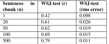
Sentences in chunk (n)

WSJ-test (r) WSJ-test (rms error)

1 0.42 0.098

20 0.61 0.026

50 0.62 0.019

100 0.69 0.015

500 0.79 0.011

Table 2: Performance of predictor on n-sentence chunks from WSJ-test (Correlation and rms error between actual/predicted accuracies).

rather than a single sentence. Predicting the corre-lation at chunk level is, not unexpectedly, an eas-ier problem than predicting correlation at sentence level, as the results in the first two columns of Ta-ble 2 show.

For 100-sentence chunks, we also plot the pre-dicted accuracies versus actual accuracies for the WSJ-test set in Figure 1. This scatterplot brings to light an artifact of using correlation metric (r) for evaluating our predictor’s performance. Although our objective is to improve correlation between ac-tual and predicted F-scores, the correlation metric (r) does not tell us directly how well the predictor is

doing. In Figure 1, the system predicts that on

an average, most sentence chunks can be parsed with an accuracy of 0.9085 (which is the mean dicted F-score on WSJ-test). But the range of pre-dictions from our system [0.89,0.92] is smaller than the actual F-score range [0.86,0.95]. Hence, even though the correlation scores are high, this does not necessarily mean that our predictions are on target.

An additional metric,root-mean-square (rms) error,

which measures the distance between actual and pre-dicted F-measures, can be used to gauge the qual-ity of our predictions. For a particular chunk-size,

lowering the rms error translates into aligning the

points of a scatterplot as the one in Figure 1, closer to the x=y line, implying that the predictor is getting better at exactly predicting the F-score values. The third column in Table 2 shows the rms error for our predictor at different chunk sizes. The results using this metric also show that the prediction problem be-comes easier as the chunk size increases.

Assuming that we have the test set of WSJ sec-tion 23, but without the gold-standard trees, how can we get an approximation for the overall

accu-racy of a parserP on this test set? One possibility,

0.85 0.86 0.87 0.88 0.89 0.9 0.91 0.92 0.93 0.94 0.95

0.85 0.86 0.87 0.88 0.89 0.9 0.91 0.92 0.93 0.94 0.95

Actual Accuracy

Predicted Accuracy

per-chunk-accuracy x=y line Fitted-line

Figure 1: Plot showing Actual vs. Predicted accuracies for WSJ-test (100-sentence chunks). Each plot point represents a 100-sentence chunk.(rms error = 0.015)

0.85 0.86 0.87 0.88 0.89 0.9 0.91 0.92 0.93 0.94 0.95

0.85 0.86 0.87 0.88 0.89 0.9 0.91 0.92 0.93 0.94 0.95

Actual Accuracy

Predicted Accuracy

per-chunk-accuracy x=y line

Figure 2: Plot showing Actual vs. Adjusted Predicted accu-racies(shifting withα = 0.757, skewing withβ = 1.0)for WSJ-test (100-sentence chunks).(rms error = 0.014)

System F-measure

Charniak F-measure on WSJ-dev (baseline) 90.48 (fd) Predictor (feature weights set with WSJ-dev) 90.85 (fp) Actual Charniak accuracy 91.13 (ft)

Table 3: Comparing Charniak parser accuracy (from different systems) on entire WSJ-test corpus

24) for this purpose, and (Charniak and Johnson,

2005) as the parserP, the baseline is an F-score of

90.48 (fd), which is the actual Charniak parser

accu-racy on WSJ section 24. Instead, if we run our pre-dictor on the test set (a single chunk containing all the sentences in the test set), it predicts an F-score

of 90.85 (fp). These two predictions are listed as

the first two rows in Table 3. Of course, having the actual gold-standard trees for WSJ section 23 helps us decide which prediction is better: the actual ac-curacy of the Charniak parser on WSJ section 23 is

an F-score of 91.13 (ft), which makes our prediction

better than the baseline.

4.1 Shifting Predictions to Match Actual Accuracy

We correctly predict (in Table 3) that the

test is easier to parse than the

WSJ-dev (90.85>90.48). However, our predictor is too

conservative—the WSJ-test is actually even easier

to parse (91.13>90.85). We can fix this by

shift-ing the mean predicted F-score (which is equal to

fp) further away from the dev F-measure (fd), and

closer to the actual F-measure (ft). This is achieved

by shifting all the individual predictions by a certain amount as shown below.

Letpbe an individual prediction from our system.

The shifted predictionp0is given by:

p0=p+α(fp−fd) (1)

We can tune α to make the new mean

predic-tion (f_p0) to be equal to the actual F-measure (ft).

fp0 = fp+α(fp−fd) (2)

α = ft−fp

fp−fd

(3)

Using the F-score values from Table 3, we get an

α = 0.757 and an exact prediction of 91.13. Of

course, this is because we tune on test, so we need to validate this idea on a new test set to see if it leads to improved predictions (Section 5).

4.2 Skewing to Widen Prediction Range

Our predictor is also too conservative about its

dis-tribution(see Figure 1). It knows (roughly) which chunks are easier to parse and which are harder, but its range of predictions is lower than the range of actual F-measure scores.

We can skew individual predictions so that sen-tences predicted to be easy are re-predicted to be even easier (and those that are hard to be even

harder). For each prediction p0 (from Equation 1),

we compute

p00=p0+β(p0−fp0) (4)

We simply set β to 1.0, doubling the distance

of each predictionp0 (in Equation 1) from the

(ad-justed) mean predictionf_p0, to obtain the skewed

pre-dictionp00.

Figure 2 shows how the points representing 100-sentence chunks in Figure 1 look after the

predic-tions have been shifted (α = 0.757) and skewed

(β = 1.0). These two operations have the desired

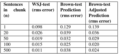
Sentences in chunk (n)

WSJ-test (rms error)

Brown-test Prediction (rms error)

Brown-test Adjusted Prediction (rms error)

1 0.098 0.129 0.139

20 0.026 0.039 0.036

50 0.019 0.032 0.029

100 0.015 0.025 0.020

500 0.011 0.038 0.024

Table 4: Performance of predictor on n-sentence chunks from WSJ-test and Brown-test (rms error between actual/predicted accuracies).

range of [0.86,0.95]. The points in the new plot (Fig-ure 2) also align closer to the “x=y” line than in the original graph (Figure 1). The rms error also drops from 0.015 to 0.014 (7% relative reduction), show-ing that the predictions have improved.

Since we use the WSJ-test corpus to tune the pa-rameter values for shifting and skewing, we need to apply our predictor on a different test set to see if we get similar improvements by using these techniques, which we do in the next section.

5 Predicting Accuracy on the Brown Corpus

The Brown corpus represents a genuine challenge for our predictor, as it presents us with the oppor-tunity to test the performance of our predictor in an out-of-domain scenario. Our predictor, trained on WSJ data, is now employed to predict the

per-formance of a WSJ-trained parserP on the

Brown-test corpus. As in the previous experiments, we use (Charniak and Johnson, 2005) trained on WSJ

sec-tions 02-21 as parserP. The feature weights for our

predictor are again trained on section 24 of WSJ, and

the shifting and skewing parameters (α = 0.757,

β = 1.0) are determined using section 23 of WSJ.

The results on the Brown-test, both the origi-nal predictions and after they have been adjusted (shifted/skewed), are shown in Table 4, at different

level of chunking. For chunks of size n > 1, the

shifting and skewing techniques help in lowering the rms error. On 100-sentence chunks from the Brown

test, shifting and skewing (α = 0.757, β = 1.0)

leads to a 20% relative reduction in the rms error. In a similar vein with the evaluation done in Sec-tion 4, we are interested in estimating the overall

ac-curacy of a WSJ-trained parser P given an

out-of-domain set such as the Brown test set (for which, at least for now, we do not have access to gold-standard

System F-measure

Baseline1 (F-measure on WSJ sec. 23) 91.13 Baseline2 (F-measure on WSJ sec. 24) 90.48

Predictor (base) 88.48

Adjusted Predictor (shifting usingα= 0.757) 86.96

Actual accuracy 86.34

Table 5: Charniak parser accuracy on entire Brown-test corpus

trees). If we use (Charniak and Johnson, 2005) as

parser P, a cheap and readily-available answer is

to approximate the performance using the Charniak parser performance on WSJ section 23, which has an F-score of 91.13. Another cheap and readily-available answer is to take the Charniak parser per-formance on WSJ section 24 with an F-score of 90.48. Table 5 lists these baselines, along with the prediction made by our system when using a single chunk containing all the sentences in the Brown test set (both base predictions and adjusted predictions,

i.e. shifting usingα = 0.757). Again, having

gold-standard trees for the Brown test set helps us decide which prediction is better. Our predictions are much closer to the actual Charniak parser performance on the Brown-test set, with the adjusted prediction at 86.96 compared to the actual F-score of 86.34.

6 Ranking Parser Performance

One of the main goals for computing F-score figures (either by traditional PARSEVAL evaluation against gold standards or by methods such as the one pro-posed in this paper) is to compare parsing accu-racy when confronted with a choice between vari-ous parser deployments. Not only are there many parsing techniques available (Collins, 2003; Char-niak and Johnson, 2005; Petrov and Klein, 2007; McClosky et al., 2006; Huang, 2008), but recent annotation efforts in providing training material for statistical parsing (LDC, 2005; LDC, 2006a; LDC, 2006b; LDC, 2006c; LDC, 2007) have compounded the difficulty of the choices (“Do I parse using parser X?”, “Do I train parser X using the treebank Y or Z?”). In this section, we show how our predictor can provide guidance when dealing with some of these choices, namely the choice of the training material to use with a statistical parser, prior to its applica-tion in an NLP task.

For the experiments reported in this paper, we

use as parser P, our in-house implementation of

speed-related enhancements (Goodman, 1997) have been applied. This choice has been made to better

reflect a scenario in which parserP would be used

in a data-intensive application such as syntax-driven machine translation, in which the parser must be able to run through hundreds of millions of training words in a timely manner. We use the more accurate, but slower Charniak parser (Charniak and Johnson,

2005) as the reference parser P_ref in our predictor

(see Section 3.3). In order to predict the Collins-style parser behavior on the ranking task, we use the same predictor model (including feature weights and adjustment parameters) that was used for predicting Charniak parser behavior on the Brown corpus (Sec-tion 5).

We compare three training scenarios that make for three different parsers:

(1) PW SJ - trained on sections 02-21 of WSJ.

(2) PN ews - trained on the union of the English

Chinese Translation Treebank (LDC, 2007) (news stories from Xinhua News Agency translated from Chinese into English) and the English Newswire Translation Treebank (LDC, 2005; LDC, 2006a; LDC, 2006b; LDC, 2006c) (An-Nahar new stories translated from Arabic into English).

(3) PW SJ−N ews - trained on the union of all the

above training material.

When comparing the performance of these three parsers on a development set from WSJ (section 0),

we get the following F-scores.5

Parser WSJ (sec. 0) Accuracy (F-scores)

PW SJ 88.25

PN ews 83.00 PW SJ−N ews 88.00

Consider now that we are interested in compar-ing the parscompar-ing accuracy of these parsers on a do-main completely different from WSJ. The ranking PW SJ>PW SJ−N ews>PN ews, given by the

evalua-tion above, provides some guidance, but is this

guid-ance accurate? The intuition here is that the

in-formation that we already have about the new do-main of interest (which implicitly appears in texts

5

Because of tokenization differences between the different treebanks involved in these experiments, we have to adopt a to-kenization scheme different from the one used in the Penn Tree-bank, and therefore the F-scores, albeit in the same range, are not directly comparable with the ones in the parsing literature.

Parser Xinhua News Prediction (F-scores)

Xinhua News Accuracy (F-scores)

PW SJ 85.1 79.14

PN ews 87.0 84.84

PW SJ−N ews 89.4 85.14

Table 6: Performance of predictor on the Xinhua News domain, com-pared with actual F-scores.

extracted from this domain), can be used to

bet-ter guide this decision. Our predictor is able to

capitalize on this information, and provide domain-informed guidance for choosing the most accurate parser to use with the new data, which in this case relates to choosing the best training strategy for the

parserP. If we consider as our domain of interest,

news stories from Xinhua News Agency, then using our predictor on a chunk of 1866 sentences from this domain gives the F-scores shown in the second col-umn of Table 6.

As with the previous experiments, we can com-pute the actual PARSEVAL F-scores (using gold-standard) for this particular 1866-sentence test set, as it happens to be part of the English Chinese Trans-lation Treebank (LDC, 2007). These F-score fig-ures are shown in the third column of Table 6. As these results show, for this particular domain the

cor-rect ranking is PW SJ−N ews>PN ews>PW SJ, which

is exactly the ranking predicted by our method, with-out the aid of gold-standard trees.

We observe that even though the system predicts the ranking correctly, the predictions in the Xinhua News domain might not be as accurate in compar-ison to the predictions on Brown corpus (predicted F-score = 86.96, actual F-score = 86.34). One pos-sible reason for this lower accuracy is that we use the same prediction model without optimizing for the particular parser on which we wish to make pre-dictions. Still, the model was able to make distinc-tions between multiple parsers for the ranking task correctly, and decide the best parser to use with the given data. We believe this to be useful in typical NLP applications which use parsing as a component, and where making the right choice between differ-ent parsers can affect the end-to-end accuracy of the system.

7 Conclusion

where it is accurate enough to be useful in a

va-riety of natural language applications. However,

due to large variations in the characteristics of the domains for which these applications are devel-oped, estimating parsing accuracy becomes more involved than simply taking for granted accuracy estimates done on a certain well-studied domain, such as WSJ. As the results in this paper show, it is possible to take into account these variations in the domain characteristics (encoded in our predictor as text-based, syntax-based, and agreement-based features)—to make better predictions about the ac-curacy of certain statistical parsers (and under dif-ferent training scenarios), instead of relying on accu-racy estimates done on a standard domain. We have provided a mechanism to incorporate these domain variations for making predictions about parsing ac-curacy, without the costly requirement of creating human annotations for each of the domains of inter-est. The experiments shown in the paper were lim-ited to readily available statistical parsers (which are widely deployed in a number of applications), and certain domains/genres (because of ready access to gold-standard data on which we could verify tions). However, the features we use in our predic-tor are independent of the particular type of parser or domain, and the same technique could be applied for making predictions on other parsers as well.

There are many avenues for future work opened up by the work presented here. The accuracy of the predictor can be further improved by incorporating more complex syntax-based features and multiple-agreement features. Moreover, rather than predict-ing an intrinsic metric such as the PARSEVAL F-score, the metric that the predictor learns to pre-dict can be chosen to better fit the final metric on which an end-to-end system is measured, in the style of (Och, 2003). The end-result is a finely-tuned tool for predicting the impact of various parser design de-cisions on the overall quality of a system.

8 Acknowledgements

We wish to acknowledge our colleagues at ISI, who provided useful suggestions and constructive criti-cism on this work. We are also grateful to all the reviewers for their detailed comments. This work was supported in part by NSF grant IIS-0428020.

References

Joshua Albrecht and Rebecca Hwa. 2007. Regression for sentence-level mt evaluation with pseudo references. InProc. of ACL.

Eleftherios Avramidis and Philipp Koehn. 2008. Enrich-ing morphologically poor languages for statistical ma-chine translation. InProc. of ACL.

Michiel Bacchiani, Michael Riley, Brian Roark, and Richard Sproat. 2006. MAP adaptation of stochastic grammars. Computer Speech & Language, 20(1). Daniel M. Bikel. 2002. Design of a multi-lingual,

parallel-processing statistical parsing engine. InProc. of HLT.

E. Black, S. Abney, D. Flickinger, C. Gdaniec, R. Gr-ishman, P. Harrison, D. Hindle, R. Ingria, F. Jelinek, J. Klavans, M. Liberman, M. Marcus, S. Roukos, B. Santorini, and T. Strzalkowski. 1991. A proce-dure for quantitatively comparing the syntactic cover-age of english grammars. InProc. of Speech and Nat-ural Language Workshop.

Eugene Charniak and Mark Johnson. 2005. Coarse-to-fine n-best parsing and MaxEnt discriminative rerank-ing. InProc. of ACL.

Eugene Charniak, Kevin Knight, and Kenji Yamada. 2003. Syntax-based language models for statistical machine translation. InProc. of MT Summit IX. IAMT. Ciprian Chelba and Frederick Jelinek. 1998. Exploiting syntactic structure for language modeling. InProc. of ACL.

Michael Collins, Philipp Koehn, and Ivona Kucerova. 2005. Clause restructuring for statistical machine translation. InProc. of ACL.

Michael Collins. 2003. Head-driven statistical models for natural language parsing. Computational Linguis-tics, 29(4).

Michel Galley, Mark Hopkins, Kevin Knight, and Daniel Marcu. 2004. What’s in a translation rule? InProc. of HLT/NAACL.

Michel Galley, Jonathan Graehl, Kevin Knight, Daniel Marcu, Steve DeNeefe, Wei Wang, and Ignacio Thayer. 2006. Scalable inferences and training of context-rich syntax translation models. In Proc. of ACL.

Daniel Gildea. 2001. Corpus variation and parser perfor-mance. InProc. of EMNLP.

Joshua Goodman. 1997. Global thresholding and multiple-pass parsing. InProc. of EMNLP.

Ulf Hermjakob. 2001. Parsing and question classifica-tion for quesclassifica-tion answering. InProc. of ACL Work-shop on Open-Domain Question Answering.

Liang Huang, Kevin Knight, and Aravind Joshi. 2006. Statistical syntax-directed translation with extended domain of locality. InProc. of AMTA.

Liang Huang. 2008. Forest reranking: Discriminative parsing with non-local features. InProc. of ACL. Dan Klein and Christopher D. Manning. 2003. Accurate

unlexicalized parsing. InProc. of ACL.

LDC. 2005. English newswire translation tree-bank. Linguistic Data Consortium, Catalog number LDC2005E85.

LDC. 2006a. English newswire translation tree-bank. Linguistic Data Consortium, Catalog number LDC2006E36.

LDC. 2006b. GALE Y1 Q3 release - English translation treebank. Linguistic Data Consortium, Catalog num-ber LDC2006E82.

LDC. 2006c. GALE Y1 Q4 release - English translation treebank. Linguistic Data Consortium, Catalog num-ber LDC2006E95.

LDC. 2007. English chinese translation tree-bank. Linguistic Data Consortium, Catalog number LDC2007T02.

Ding Liu and Daniel Gildea. 2007. Source-language fea-tures and maximum correlation training for machine translation evaluation. InProc. of NAACL-HLT. Daniel Marcu, Wei Wang, Abdessamad Echihabi, and

Kevin Knight. 2006. Spmt: Statistical machine trans-lation with syntactified target language phraases. In Proc. of EMNLP.

Mitchell P. Marcus, Mary Ann Marcinkiewicz, and Beat-rice Santorini. 1993. Building a large annotated cor-pus of English: The Penn Treebank. Computational Linguistics, 19(2).

David McClosky, Eugene Charniak, and Mark Johnson. 2006. Reranking and self-training for parser adapta-tion. InProc. of COLING-ACL.

Franz Joseph Och. 2003. Minimum error rate training in machine translation. InProc. of ACL.

Slav Petrov and Dan Klein. 2007. Improved inference for unlexicalized parsing. InProc. of HLT/NAACL. Brian Roark. 2001. Probabilistic top-down parsing

and language modelling. Computational Linguistics, 27(2).

A.J. Smola and B. Schoelkopf. 1998. A tutorial on sup-port vector regression.NeuroCOLT2 Technical Report NC2-TR-1998-030.

Radu Soricut. 2006. Natural Language Generation us-ing an Information-Slim Representation. Ph.D. thesis, University of Southern California,.