Control of Marangoni Convection in a Variable-Viscosity Fluid Layer with Deformable Surface

(1)

Control of Marangoni Convection in a

Variable-Viscosity Fluid Layer with Deformable

Surface

Seripah Awang Kechil

1

_{and Ishak Hashim}

2∗

Abstract—The effectiveness of a proportional

feed-back control to suppress the Marangoni instability in a variable-viscosity fluid layer with a deformable free upper surface is investigated. Viscosity variation and deformable free surface have destabilizing effects on the stability limit. The stability thresholds for the short-scale mode are strongly dependent on viscos-ity variation and controller gain while the stabilviscos-ity thresholds for the long-scale mode are greatly influ-enced by gravity and surface deformation. The feed-back control strategy through thermal perturbation in the boundary data is shown effective in suppress-ing the Marangoni convection and delaysuppress-ing the onset of instability.

Keywords: Marangoni convection, feedback control, variable viscosity, deformable surface, instability

1 Introduction

Surface-tension-driven and buoyancy-driven convective flows have long been studied since the pioneering works of Benard [1], Rayleigh [2] and Pearson [3]. Convective flows are of practical importance in material processing technology in industrial applications. The industrial need has motivated extensive theoretical, experimental and numerical investigations to clarify the onset mechanism of the instability. Since convective flows are undesirable, it is beneficial to have a means to control the convec-tive motions and achieve the preferable flow characteris-tics. Tang and Bau [4, 5] successfully applied the feed-back control strategy to suppress the Rayleigh-Bénard convection. Bau [6] demonstrated that a proportional feedback control was effective in delaying the onset of convection in Marangoni-Bénard problems of Pearson [3] and Takashima [13, 14]. Arifin et al. [7] investigated the effect of a feedback control on Marangoni-Bénard convec-tion for a free-slip bottom.

The stabilising effects of magnetic field and rotation on

∗_{Supported by the Ministry of Sciences, Technology &} Innova-tion (MOSTI) of Malaysia under grant no 06-01-02-SF0115 and the Universiti Teknologi MARA. 1_{Centre of Mathematical Sciences,}

Universiti Teknologi MARA, 40450 Shah Alam Selangor. Email: [email protected]_{School of Mathematical Sciences,}

Uni-versiti Kebangsaan Malaysia, 43600 UKM Bangi Selangor. Tel: +603 89215758 Fax: +603 89254519 Email: ishak [email protected]

Marangoni convection have been analysed by Hashim and Arifin [8], Hashim and Sarma [9, 10] and Sarma and Hashim [11]. The aforementioned studies only dealt with fluids with invariant viscosity. However, viscos-ity of most fluids is known to decrease with temper-ature [15] and has a destabilising effect on convection [16, 17, 18, 19, 20]. Slavtchev and Ouzounov [19] stud-ied the destabilising effect of temperature-dependent vis-cosity in the Marangoni problem in microgravity. The effects of viscosity variation, gravity waves and surface deformation on Marangoni instability has been analysed by Kalitzova-Kurteva et al. [20].

In this paper, we will demonstrate the possibility to al-ter the stability characal-teristics in Marangoni problem of a temperature-dependent-viscosity fluid layer. The ther-mal proportional feedback control is employed to sup-press the intensity of Marangoni convection. We will show that the critical Marangoni number can be increased to delay the onset of convection and appreciably to sta-bilise the liquid layer.

2 Problem Formulation

2.1 Governing equations

Consider a horizontal layer of quiescent fluid of depthd

on a rigid heat-conducting wall with a free upper sur-face. Variations of the dynamic viscosityµ and the sur-face tensionσof the fluid with temperature are assumed exponential and linear, respectively,

µ = µ0exp [−γ(T−T0)], (1)

σ = σ0−ε(T−T0), (2)

whereT is the temperature of the liquid,µ0 andσ0

cor-respond to values at a reference temperature T0, γ and

ε, which are positive for most fluids, correspond to the rate of change of the dynamic viscosity and the surface tension with temperature, respectively. Other physical properties of the liquid are assumed constant. The sur-face of the horizontal wall coincides with the xy-plane and thez-coordinate measures the vertical distance from the wall.

In the reference state, the fluid is at rest with the pressure

(2)

and the liquid temperature are

pst = pg+ρg(d−z), (3)

Tst = Tw−βz, (4)

wherepgis the gas pressure,ρthe density,g the acceler-ation due to gravity,Tw the temperature at the wall and

β > 0. When motion sets in, the velocityv = (u, v, w), pressurepand temperatureT fields obey the usual bal-ance equations of mass, momentum and energy [20],

∇ ·v = 0, (5)

ρ

_∂_v

∂t + (v· ∇)v

= _−∇p+_{∇ ·}(2µDv) +ρg,(6)

∂T

∂t + (v· ∇)T = χ∇

2

T, (7)

where χ is the thermal diffusivity, g(0,0,₋g) the gravi-tational acceleration, andDthe deformation rate tensor.

2.2 Linearised controlled problem

We wish to extend the work of Kalitzova-Kurteva et al. [20] by applying a simple control mechanism of Bau [6] to suppress the intensity of convection and subsequently delay the onset of convection. The stability of the liquid system under controlled environment will be studied by applying a very simple linear active control of propor-tional feedback. Thermal control strategy can be easily applied and thus simplify the problem of mathematical formulation to a large extent where a slight modification in the temperature field does not alter the internal mech-anism in the system. The temperature perturbation field is measured by a continuous distribution of sensors em-bedded in a plane parallel to the xy-plane at a chosen level. Each sensor emits signals to a thermal actuator positioned directly beneath it on the heated surface. By the proportional feedback rule, the actuator modifies the heated surface temperature using a proportional relation-ship between the temperature at the upper surface, z=1, and the lower surface, z=0, [6]

T(x, y,0, t) = T(x, y,0)

−K[T(x, y,1, t)₋T(x, y,1)], (8)

or equivalently

T′₍_{x, y,}₀_{, t}_{) =}₋_KT′₍_{x, y,}₁_{, t}₎_, ₍₉₎

whereK is the controller gain andT′ _{denotes the} devia-tion of the fluid’s temperature from its conductive value.

The stability of the problem will be investigated by per-forming a linear stability analysis. In formulation of the dynamic conditions in the liquid system, the governing equations and boundary conditions are linearised. We consider a small disturbance,

(w′_{, T}′_{, ζ}_{) =} _[₋_W₍_z₎_,_Θ(_z₎_{, Z}_{] exp}

i(αxx+αyy) +ωt

, (10)

where ζ = ζ(x, y, t) is the deviation from the flat free surface, W(z), Θ(z) and Z the amplitudes, α =

α2

x+α

2

y

1/2

the wave number, andωthe time constant.

Substituting (10) into the linearised equations from (5)– (7) and introducing the quantitiesd,d2

/χ,χ/d,µ0χ/d 2

, andβdas the scales for distance, time, velocity, pressure, and temperature, respectively, yield [20]

f(z)

D2

−α2

+N2

+ 2N D

D2

−α2

+2N2

α2

W = Pr−1

ω D2

−α2

W, (11)

ω− D2

−α2

Θ =−W, (12)

whereD= d/dz.

The boundary conditions at both surface boundaries,z= 0 andz= 1, comprise of,

W(0) =DW(0) = 0, (13)

W(1) +ωZ= 0, (14)

f(1)

D2

−3α2

DW(1) +N D2

+α2

W(1)

+α

2

Bo +α2

Z Cr = Pr

−1

ωDW(1), (15)

f(1) D2

+α2

W(1)₋α2

M a[θ(1)₋Z] = 0, (16)

DΘ(1) + Bi [Θ(1)−Z] = 0, (17)

while the uniform temperature boundary at the wall sur-face,z= 0, is reinstated to include a controller rule with gainK,

Θ(0) +KΘ(1) = 0. (18)

The dimensionless parameters are M a = εβd2

/χµ0 the

Marangoni number, Cr = µ0χ/σdthe Crispation

num-ber, Bo =ρgd2

/σ0the Bond number, Bi =hd/λthe Biot

number, Pr =µ0/ρχthe Prandtl number and N =γβd

the viscosity parameter where λis the thermal conduc-tivity of the fluid and h is the heat transfer coefficient between the liquid and the gas phase at the upper free surface. The function f(z) is given by

f(z) = exp

N

z₋1 + T0−Ts

βd

. (19)

In relation with some previous works of controlled and uncontrolled systems, when N = 0, the system (11)– (18) reduces to a system of a constant-viscosity liquid with the application of a feedback control considered by Bau [6]. For K = 0 and N = 0 the system coincides with a constant-viscosity liquid of Marangoni problem of Takashima [13]. WhenK= 0 andCr= 0 we recover the variable-viscosity Marangoni problem of Slavtchev and Ouzounov [19] with the nondeformable free surface and settingK= 0,N = 0 andCr= 0, we recover the classi-cal Marangoni problem of Pearson [3].

(3)

Since the dynamic viscosity of the fluid varies with temperature, the reference temperature for a variable-viscosity fluid can be taken as temperature at the bot-tom boundary µw, temperature at the upper free sur-face µs or mean value of viscosities at both boundaries

µ = (µw+µs)/2 [19, 20]. The system (11)–(18) will be solved for M as, the Marangoni number corresponds to µs. Then, M as will be used to determine the mean Marangoni numberM agiven by

M a= 2εβd

2

χ(µs+µw)

= 2M as

1−exp(−N), (20)

in relation to the modified Crispation number for the mean value of viscosities,

Cr= χ(µs+µw) 2σd =

[1₋exp(₋N)]Cr

2 . (21)

Thus, our conclusions of the Marangoni instability will be based on the marginal stability curvesM a.

We restrict to the case of a deformable surface Cr 6= 0 and consider the influences of no gravity Bo = 0, grav-ity waves Bo = 0.1 and the heat transfer mechanism at the free upper surface Bi = 0 and Bi = 0.1. Bo = 0.1 is representative for thin layers of some oils used in ex-periments on earth [20]. Bi = 0 represents a thermally perfectly insulated free surface and is considered as the most unstable situation since the whole thermal energy communicated in the system remains inside the liquid layer. We also include Bi = 0.1 since the Biot number Bi is at most 0.1 for a thin layer of liquid.

3 Results and discussion

We seek a closed form solution for the marginal stability curves of the steady (ω = 0) Marangoni convection and by setting ω = 0 in (11), the solution for W(z) which satisfies the boundary conditions (13) and (14) is,

W(z) = A1

[exp(k1z)−exp(k2z)] cos(k3z)

−[A2exp(k1z)−A3exp(k2z)] sin(k3z) ,

(22)

whereA1is an arbitrary constant andk1, k2, k3, k, A2and

A3 are given by,

k1 = −

N 2 + 1 √ 2 k2

+α2

+N

2

4

1/2

, (23)

k2 = −

N 2 − 1 √ 2 k2

+α2

+N

2

4

1/2

, (24)

k3 =

1 √ 2 k2 − α2 +N 2 4

1/2

, (25)

k =

"

α2+N

2

4

2

+α2N2

#1/4

, (26)

A2 = cotk3+

(k2−k1) exp (k2−k1)

k3[1−exp (k2−k1)]

, (27)

A3 = cotk3+

k2−k1

k3[1−exp (k2−k1)]

. (28)

Substituting W(z) in (12), the complete solution for the temperature is

Θ(z) = F1sinh(αz) +F2cosh(αz) + Θp(z), (29)

whereF1andF2are to be determined from the boundary

conditions (17) and (18). Θp(z) denotes the particular solution corresponding to the nonhomogeneous equation involvingW(z). Thus,

Θp(z) = A1

n

[C1exp (k1z) +C2exp (k2z)] cos(k3z)

+ [C3exp (k1z) +C4exp (k2z)] sin (k3z)

o

,

(30)

where

C1 =

2A2k1k3+ k 2 1−k

2 3−α

2

4k2 1k

2 3+ (k

2 1−k

2 3−α

2₎2 , (31)

C2 = −

2A3k2k3+ k22−k 2 3−α

2

4k2 2k

2 3+ (k

2 2−k

2 3−α

2₎2 , (32)

C3 =

2k1k3−A2 k 2 1−k

2 3−α

2

4k2 1k

2 3+ (k

2 1−k

2 3−α

2₎2 , (33)

C4 = −

2k2k3−A3 k 2 2−k

2 3−α

2

4k2 2k

2 3+ (k

2 2−k

2 3−α

2₎2 . (34)

The expressions forW(z) and the derivatives ofW(z) and Θp(z) at z = 1 for the determination of the remaining unknown quantities are listed as follows,

W(1) = A1

h

(expk1−expk2) cosk3

−(A2expk1−A3expk2) sink3

i

, (35)

D2

W(1) = A1

nh

k2 1−k

2

3−2A2k1k3

expk1

+ 2A3k2k3−k 2 2+k

2 3

expk2

i

cosk3

+h A2k 2 3−A2k

2

1−2k1k3

expk1

+ 2k2k3+A3k 2 2−A3k

2 3

expk2

i

sink3

o

,

(36)

D3

W(1) = A1

nh

k3 1−3k

2

3k1−3A2k3k 2 1

+A2k 3 3

expk1+ 3k 2

3k2+ 3A3k3k 2 2

−k3 2−A3k

3 3

expk2

i

cosk3

+h k3

3+ 3A2k 2

3k1−3k3k 2 1−A2k

3 1

expk1

+ 3k3k 2 2−k

3 3+A3k

3 2

−3A3k 2 3k2

expk2

i

sink3

o

(37)

(4)

Θp(1) = A1

h

(C1expk1+C2expk2) cosk3

+ (C3expk1+C4expk2) sink3

i

, (38)

DΘp(1) = A1

n

(C1k1+C3k3) expk1

+ (C2k2+C4k3) expk2cosk3

+

(C3k1−C1k3) expk1

+ (C4k2−C2k3) expk2

sink3

o

. (39)

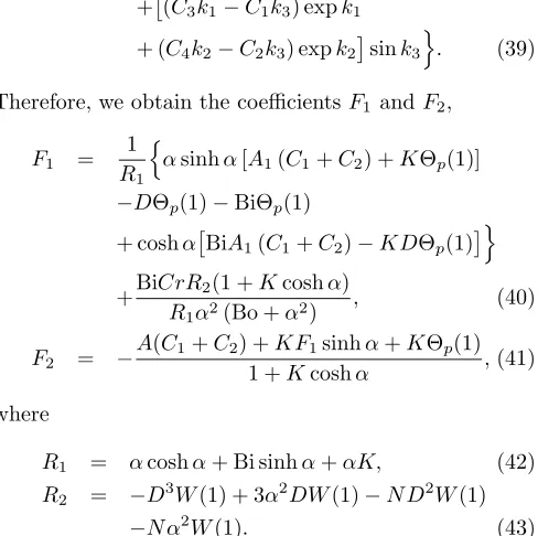
Therefore, we obtain the coefficientsF1 andF2,

F1 =

1

R1

n

αsinhα[A1(C1+C2) +KΘp(1)]

−DΘp(1)₋BiΘp(1) + coshα

BiA1(C1+C2)−KDΘp(1)

o

+BiCrR2(1 +Kcoshα)

R1α2(Bo +α2)

, (40)

F2 = −

A(C1+C2) +KF1sinhα+KΘp(1)

1 +Kcoshα ,(41)

where

R1 = αcoshα+ Bi sinhα+αK, (42)

R2 = −D 3

W(1) + 3α2

DW(1)₋N D2

W(1) −N α2

W(1). (43)

The magnitude of the surface deflection Z can be cal-culated from (15). From boundary condition (16), we obtain an expression for M asin terms of α, K, N, Cr,Bi and Bo which can be conveniently written in the form

M as = −

R1 Bo +α 2

α2

W(1) +D2

W(1)

R3

,(44)

where

R3 = αcoshα

n

α2

Θp(1) Bo +α2

−h3α2

DW(1)₋D3

W(1)₋N D2

W(1)

−N α2

W(1)iCro₋α2

sinhαDΘp(1) Bo +α2

−α3

A1 Bo +α 2

(C1+C2)

+αKCrhD3

W(1)₋3α2

DW(1)

+N D2

W(1) +N α2

[image:4.612.50.294.106.349.2]

W(1)i. (45)

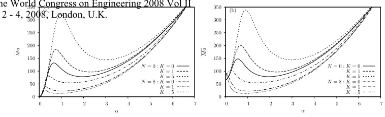
Fig. 1 shows the marginal stability curves for a case of a deformable surface Cr = 0.001 and Bi = 0 for some parameters values of Bo, N andK. Each curve has two local minima, one at α = 0 of long-scale mode and the other one atα >0 of the short-scale mode. In Fig. 1(a), when Bo = 0 the global minima are at α= 0 indicating that only the long-scale mode dominates where the con-troller gain K is not effective. When the gravity waves are considered Bo = 0.1, as shown in Fig. 1(b), the local

minimum atα= 0 has a nonzero mean Marangoni num-berM a. As the value of the controller gainK increases, the marginal stability profile increases but as the viscosity parameter increases, the marginal profile decreases. The global minima for constant-viscosity fluid are at α = 0 while the global minima for a variable-viscosity fluid of

N = 8 are atα >0.

Figs. 2 and 3 show the effects of viscosity variation N

and controller gainK on M ac and αc for Bo = 0.1 and

Cr = 0.001. In Fig. 2, there exists a critical value of viscosity parameter, say N∗ _{where when}_{N < N}∗_, _{M a}_c increases and when N > N∗_, _{M a}_c _decreases. _{M a}_c _for Bi = 0.1 is slightly higher than M ac for Bi = 0. The long-scale mode occurs when N < N∗ _{while the} short-scale dominates when N > N∗ _and _α_c _{decreases as} _N increases. When N =N∗_{, both modes co-exist marked} by discontinuous jumps (vertical lines) of αc from zeros to nonzero values. AsK increases, the effect of Bi onαc weakens. In Fig. 3, there exists a critical value of con-troller gain, sayK∗ _{where when}_{K < K}∗_,_{M a}

c increases in a short-scale mode but when K > K∗_, _{M a}

c is insen-sitive of K in a long-scale mode. WhenK =K_∗, both modes occur with transitions from an increasingM ac to a stableM ac and from a short-scale mode to a long-scale mode.

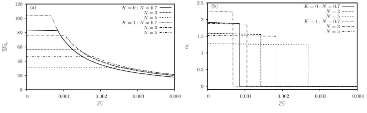
The effect of deformable surface on the marginal curves,

M acandαcare depicted in Fig. 4 and 5. The curve for a deformable surfaceCr6= 0 differs fundamentally from the curve for a nondeformable surfaceCr = 0. There exist two local minima for Cr 6= 0 instead of one minimum for the case Cr = 0. When the surface is increasingly deformed, the minimum at α > 0 is invariant but the minimum atα= 0 decreases. There exists a value ofCr∗

to mark the transition from invariantM acto a decreasing

M ac as well as the transition from the short-scale mode to a long scale mode. When Cr < Cr∗, there is a weak effect of Cr on M ac but strong effects ofK and N on

M ac. When Cr > Cr∗ and increases, M ac decreases, long-scale mode dominates and the effects of K and N

weaken.

Viscosity variation and deformable surface inhibit convec-tive motion and have destabilizing effects on the stability thresholds. The use of a proportional feedback control is effective in increasing the criticalM acand stabilising the liquid layer.

4 Conclusions

Proportional feedback control has been used to in-vestigate and suppress the Marangoni instability in a temperature-dependent-viscosity fluid layer with a de-formable upper surface. Viscosity variation and de-formable surface have destabilising effects on the stabil-ity thresholds and the use of feedback control is shown effective in suppressing the Marangoni convection in a

(5)

K= 5

K= 1

N= 8 :KK= 0= 5

K= 1

N= 0 :K= 0

(a)

α

M

a

7 6 5 4 3 2 1 0 350

300

250

200

150

100

50

0 K= 5

K= 1

N= 8 :KK= 0= 5

K= 1

N= 0 :K= 0

(b)

α

M

a

7 6 5 4 3 2 1 0 350

300

250

200

150

100

50

[image:5.612.103.482.18.134.2]

0

Figure 1: Marginal curves (a) Bo = 0 (b) Bo = 0.1 for Bi = 0,Cr= 0.001 and variousN andK.

temperature-dependent-viscosity liquid layer.

References

[1] B´enard, H., “Les tourbillons cellulaires dans une nappe liquide,” Rev G´en Sci Pures Appl, 11, pp. 1261-1271, 1900.

[2] Rayleigh, L., “On convection currents in a horizontal layer of fluid when the higher temperature is on the other side,”Philo Mag, 32, pp. 529–543, 1916.

[3] Pearson J.R.A., “On convection cells induced by sur-face tension,”J Fluid Mech, 4, pp. 489–500, 1958.

[4] Tang J., Bau H.H., “Feedback control stabilization of the no-motion state of a fluid confined in a hor-izontal, porous layer heated from below,” J Fluid Mech, 257, pp. 485–505, 1993.

[5] Tang J., Bau H.H., “Numerical investigation of the stabilization of the no-motion state of a fluid layer heated from below and cooled from above,”Phys Flu-ids, 10, pp. 1597–1610, 1998.

[6] Bau H.H., “Control of Marangoni-B´enard convec-tion,”Int J Heat Mass Transfer, 42, pp. 1327–1341, 1999.

[7] Arifin N.M., Nazar R.M., Senu N., “Feedback con-trol of the Marangoni-B´enard Instability in a fluid layer with a free-slip bottom,”J Phys Soc Japan, 76 pp. 014401, 2007.

[8] Hashim I., Arifin N.M., “Oscillatory Marangoni con-vection in a conducting fluid layer with a deformable free surface in the presence of a vertical magnetic field,”Acta Mech, 164, pp. 199–215, 2003.

[9] Hashim I., Sarma W., “On the onset of Marangoni convection in a rotating fluid layer,” J Phys Soc Japan, 75, pp. 035001, 2006.

[10] Hashim I., Sarma W., “On oscillatory Marangoni convection in a rotating fluid layer subject to a uni-form heat flux from below,”Int Commun Heat Mass Transfer, 34, pp. 225–230, 2007) .

[11] Sarma W., Hashim I., “On oscillatory Marangoni convection in rotating fluid layer with flat free sur-face subject to uniform heat flux from below,”Int J Heat Mass Transfer, 50, pp. 4508–4511, 2007.

[12] Schwabe D., “Marangoni effects in crystal growth melts,”Physico Hydrodyn, 2, pp. 263281, 1981.

[13] Takashima M., “Surface tension driven instability in a horizontal liquid layer with a deformable free sur-face, I. Stationary convection,” J Phys Soc Japan, 50, pp. 2745–2750, 1981.

[14] Takashima M., “Surface tension driven instability in a horizontal liquid layer with a deformable free sur-face, II. Overstability,” J Phys Soc Japan, 50, pp. 2751–2756, 1981.

[15] Griffiths R.W., “Thermals in extremely viscous flu-ids, including the effects of temperature-dependent viscosity,”J Fluid Mech, 166, pp. 115–138, 1986.

[16] Selak R., Lebon G., “Benard-Marangoni thermo-convective instability in presence of a temperature-dependent viscosity,”J Phys II France, 3, pp. 1185-1199, 1993.

[17] Hannaoui M., Lebon G., “B´enard-Marangoni insta-bility in an electrically conducting fluid layer with temperature-dependent viscosity under a magnetic field,” J Non-equilibrium Thermodyn, 20, pp. 350– 358, 1995.

[18] Kozhoukharova Zh., Roze C., “Influence of the sur-face deformability and variable viscosity on buoyant-thermocapillary instability in a liquid layer,” Euro-pean Phys J, B, pp. 125–135, 1999.

[19] Slavtchev S., Ouzounov V., “Stationary Marangoni instability in a liquid layer with temperature-dependent viscosity in microgravity,” Microgravity Q, 4, pp. 33–38, 1994.

[20] Kalitzova-Kurteva P.G., Slavtchev S.G., Kurtev I.A., “Stationary Marangoni instability in a liquid layer with temperature-dependent viscosity and de-formable free surface,”Microgravity Sci Technol, Int J Microgravity Res Appl, 9, pp. 257–263, 1996.

(6)

K= 5

K= 1

Bi = 0.1 :KK= 0= 5

K= 1

Bi = 0 :K= 0

(a)

N

M

ac

10 8 6 4 2 0 90

80

70

60

50

40

30

20

10

0 K= 5

K= 1

Bi = 0.1 :KK= 0= 5

K= 1

Bi = 0 :K= 0

(b)

N

αc

10 8 6 4 2 0 2 1.8 1.6 1.4 1.2 1 0.8 0.6 0.4 0.2 0

Figure 2: Effect ofN on (a)M ac (b)αc for Bo = 0.1,Cr= 0.001, Bi = 0,0.1 and K= 0,1,5.

N= 5

N= 4

N= 3 (a)

K

M

ac

6 5 4 3 2 1 0 90

80

70

60

50

40

30

N= 5

N= 4

N= 3 (b)

K

αc

6 5 4 3 2 1 0 2

1.5

1

0.5

0

Figure 3: Effect ofKon (a)M ac (b)αc for Bo = 0.1,Cr= 0.001, Bi = 0 and variousN.

Cr= 0.01

Cr= 0.002

Cr= 0.001

Cr= 0Cr.0008= 0 (a)

α

M

a

4 3

2 1

0 200

150

100

50

0 Cr= 0.01

Cr= 0.002

Cr= 0.001

Cr= 0Cr.0008= 0 (b)

α

M

a

4 3

2 1

0 250

200

150

100

50

[image:6.612.116.483.41.155.2]

0

Figure 4: Marginal curves (a)K= 0 (b) K= 1 for Bi = 0, Bo = 0.1,N = 1.5 and variousCr.

N= 5

N= 3

K= 1 :N= 0.7

N= 5

N= 3

K= 0 :N= 0.7

(a)

Cr

M

ac

0.004 0.003

0.002 0.001

0 120

100

80

60

40

20

0

N= 5

N= 3

K= 1 :NN= 0= 5.7

N= 3

K= 0 :N= 0.7

(b)

Cr

αc

0.004 0.003

0.002 0.001

0 2.5

2

1.5

1

0.5

0

Figure 5: Effect ofCr on (a)M ac (b)αc for Bi = 0, Bo = 0.1 and variousN andK.

[image:6.612.115.480.212.325.2] [image:6.612.116.484.386.495.2] [image:6.612.115.483.558.672.2]