Abstract—A hierarchical and modular modeling methodology for specifying urban traffic systems (UTS) for multi-agent based micro-simulation is presented. A multi-level Petri net based formalism, named nLNS is used for describing the structure of the UTS and the components behavior. Structural information regards the network topology, geographical information, and transit signs (traffic lights, speed limit, etc.). The behavioral part concerns the road network users, the traffic lights, and the pedestrians. Both the structure and behaviors are represented in a 3LNS model and then translated into a multi-agent architecture. The first level describes the traffic network; the second level models the behavior of diverse road network users considered as agents, and the third level specifies detailed procedures performed by the agents, namely travel plans, tasks, etc.
Index Terms—Urban traffic systems; Hierarchical modeling; Multi-agent based micro-simulation; Multi-level Petri nets.
I. INTRODUCTION
Nowadays the UTS are being widely studied for improving the travel time and fuel consumption of users and reducing the pollution [1]. Most of this system analysis is done by model based micro-simulation, which is an approach widely adopted because it represents more accurately the car behavior, traffic light control polices, traffic densities, vehicles flow, etc. [2][12]. The models supporting micro-simulation must capture detailed information about the UTS components, namely the diverse kind of vehicles, length of streets and number of lanes, and signaling.
In the literature there exist several proposals for model based micro-simulation. In [5] and [7] the UTS microscopic and macroscopic information is represented in a modular way using hybrid Petri nets (PN); however the decision making level cannot be represented in a straight way. Cell-DEVS is another formal tool presented in [14] that allows describing formally a system based on event-oriented or time-oriented approaches. In [10] a hierarchical model using Cell-DEVS for UTS modeling is proposed, allowing evaluating intelligent transport systems (ITS). Cell-DEVS is based on cellular automata to represent the movement of the objects; however it has been shown in [4] that cellular automata are inadequate to represent moving objects yielding modeling errors introduced by the users when synchronous updating is required.
Manuscript received July 30, 2008. This work was supported by CONACYT with grant No. 180892from the same Council.
E. López-Neri, A. Ramírez-Treviño and E. López-Mellado are with CINVESTAV, Unidad Guadalajara, Zapopan, 45015, México (e-mail: [email protected])
The microscopic UTS models are more realistic when the roads and user behavior are described based on the multi-agent paradigm [8]. In addition, multi-agent models can be easily adapted to include all UTS characteristics [17], allowing multiple vehicle classes and services as trains, light rail vehicles, metros, buses, taxis, limousines, etc. [9]. In [3] a meta-model framework is presented in which the streets are described as agents and the cars are messages sent and consumed by streets agents. Since that approach does not consider the cars as agents, then the car behavior and other complex behaviors cannot be captured [16].
This paper presents a UTS microscopic modeling methodology for describing the traffic network, control signals, and road network users (vehicles, pedestrians, cyclists, etc.) displacing within the network. It uses nLNS to represent UTS, and then this representation is translated into a multi-agent based model for event oriented micro simulation.
The nLNS models describe UTS using three levels. The first one is devoted to represent the system environment (the road network), the second one is devoted to represent the behavior of agents using the system environment (cars, pedestrians, etc.), and the third level describes specific behavior of the agents.
The remainder of this paper is organized as follows: section 2 summarizes the nLNS formalism; in section 3 the UTS components are presented; and finally in section 4 the UTS model components using nLNS are presented.
II. THE nLNSFORMALISM
The formalism follows the approach of nets within nets introduced by R. Valk [13], in which a two level nested net scheme called EOS (Elementary Object System) is proposed. An extension to the Valk’s technique, called nLNS, has been proposed [11]; in this section we present an overview of nLNS. A more accurate definition of the formalism is detailed in [11].
A. Definition
An nLNS model consists mainly of an arbitrary number of nets organized in n levels according to a hierarchy; n depends on the degree of abstraction that is desired in the model. A net may handle as tokens, nets of deeper levels and symbols; the nets of level n permits only symbols as tokens, similarly to CPN (Coloured PN). Interactions among nets are declared through symbolic labelling of transitions.
Fig. 1 sketches pieces of the components of a 4-LNS model. The level 1 is represented by the net NET1, the level 2 by the nets NET2,1 and NET2,2, the nets NET3,1, NET3,2,
Hierarchical Modeling of Urban Traffic Systems
for Multi-Agent Based Simulation
NET3,3, and NET3,4 compose the level 3, and the nets NET4,1, NET4,2, NET4,3 form the level 4.
a↓
NET1
NET4(2)
NET3(1)
b≡ NET2(1
b≡↓ a↑ NET4(1)
b↑
c2
c1 c3
c1
c2
c2
a≡↑
a≡↑, c↓ NET3(2)
NET2(2)
c↓↑
c↑ NET3(3)
NET4(3)
NET3(4)
a≡↑ c3
c2 c2 c1
c3
x, y
[image:2.595.70.274.85.344.2]x
Fig. 1: Piece of a 4-LNS
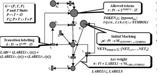
A net of level i is a tuple NETi = (typeneti, μi), where is
composed by a PN structure, the arcs weight (π((p, t), lab) or π((t, p), lab)) expressed as multi sets of variables and symbols, and a transition labelling function declaring the net interaction. μi is the marking function (see Figure 2).
Fig. 2: Example of a Net of Level i, in the n-LNS Formalism, defined as Neti=((typeneti , µi), where typeneti = (G, TOKENi, LABELi, VARi, τ, λ, π)).
A n-LNS model, called net system, is a n-tuple NS= (NET1, NET2, … NETn) where NET1 is the highest level net, and NETi = {NETi,1 , NETi,2, ... , NETi,r} is a set of r nets of level i.
The components of a model may interact among them through synchronization of transitions. The synchronization mechanism is included in the enabling and firing rules of the transitions; it establishes that two or more transitions labelled with the same symbol must be synchronized. A label may have the attributes ≡, ↓, ↑, which express local, inner, and external synchronization respectively.
B. Transition Enabling and Firing
A transition t of a net of level iNETi is enabled with respect to a label lab if:
-There exists a binding bt that associates the set of variables appearing in all π((p,t),lab).
- It must fulfil that ∀p ∈ •t, π((p, t), lab)<bt> ⊆μi(p).
(<bt> is not necessary when the level net is n).
- The conditions of one of the following cases are fulfilled: Case 1. If there is not attributes then the firing of t is autonomously performed.
Case 2. If lab has attributes one must consider the combination of the following situations:
{≡} It is required the simultaneous enabling of the transitions labelled with lab≡ belonging to other nets into the same place p’ of the next upper level net. The firing of these transitions is simultaneous and all the (locally) synchronized nets remain into p’.
{↓} It is required the enabling of the transitions labelled with lab↑ belonging to other lower level nets into •t. These transitions fire simultaneously and the lower level nets and symbols declared by π((p, t), lab)<bt> are removed.
{↑}It is required the enabling of at least one of the t’∈p’•, labelled with lab↓, of the upper level net where the NETi is contained. The firing of t provokes the transfer of NETi and symbols declared into π ((p’, t’), lab)<bt>.
The firing of transitions in all level nets modifies the marking by removing π((p, t), lab)<bt> in all the input places
and adding π((t, p), lab)<bt> to the output places.
In Figure 1, NET1 is synchronized through the transition labelled using a↓ with NET
2,2, NET3,2, NET3,4 and NET4,2 by
mean the transitions (locally synchronized) labelled with a↑; all these transitions must be enabled to fire. The simultaneous firing of the transitions removes these nets from the input places.
NET2,1, NET3,1 and NET4,1 are synchronized through the transitions labelled with b↓, b≡, b↑ respectively; the firing of
the transitions changes the marking of NET2,1 and NET3,1; NET4,1 is removed from the place of NET2,1. NET3,3 is removed from the input place of NET2,2 and NET4,3 is removed from NET3,3; this interaction is established by c↓, c↓↑, c↑, respectively.
III. URBAN TRAFFIC SYSTEM SPECIFICATION C. UTS components
The UTS entities or components are: network streets and intersections, road users (vehicle, pedestrians, cyclists, etc.), traffic signs (dynamic: traffic light, and static: speed limit sign) and individual and emergent behavior (see fig. 3).are classed into static and dynamic entities. Static entities cannot change their state, for instance traffic signals (speed limit, priority flow, etc.) or the street network. Dynamical entities or road users are objects that can move through the road network and/or change their own state, i.e., they have their own behavior (cars, pedestrians, traffic lights, variable messages signs, etc.).
[image:2.595.51.306.436.559.2]
Fig. 3: Components of an Urban Traffic System
Besides the description of the behavior of dynamic entities, the evolving rules must be also specified. These rules govern the joint behavior of entities. For instance, an evolving rule could be “two or more entities cannot be in the same space at the same time”. The evolving rules are axioms that the UTS entities cannot violate. The interaction of one road user with other road users, static components, and traffic signs leads to more complex behaviors known as emergent behaviors, for example: queues, traffic jams, gridlock, green wave, etc. [6]. This emergent behavior is not explicitly captured in the model, but it will be appear when the UTS model evolves, for instance, when a micro-simulator is used. The knowledge about queues, traffic jams, etc., allow to road users making better decisions during their execution.
D. Component Behavior
Evolving Rules
Evolving rules are the laws imposed by physical constraints of the system. The following list is the set of selected evolving rules:
E-Rule 1: Ubiquity rule. Two entities cannot occupy the same space at the same time.
E-Rule 2: Ignored entity rule. An entity cannot pass through another entity.
E-Rule 3: Network rule. An entity must travel using the road network.
E-Rule 4: Negligence rule. If one agent or more try to violate one or more of the previous rules, then the result is the crashing of the agent and other involved agents.
When an agent tries to execute one action in such a way that one evolving rule could be violated, there is a resource conflict, and then the entity must reconsider the action and select a new one, otherwise Negligence rule will be applied and the entity will crash.
Road Network
The road network is a set S of interconnected streets and intersections called segments; it contains the traveling road users the dynamic and static traffic signals. These interconnections are defined by the following two relations:
Relation 1: Parallel neighborhood
} s of neighbor adjacent
an is s , , | ) ,
{(s s s s S i j
NC= i j i j∈
Relation 2: Sequential neighborhood
} of neighbor sequential
a is , , | ) ,
{(si sj si sj S si sj
NS= ∈
Now we introduce the notions of sink and source node of a road network.
Definition 1:
Let si, sj ∈S, si, is a source node iff ¬∃sj such that (si, sj) ∈ NS. si, is a sink node iff ¬∃sj such that (sj, si) ∈NS.
Notice that using the NC and NS relations, the intersection can be represented easily.
Driver rules
Additionally, there exist some traffic policies that a typical vehicle driver must follow, for instance:
B-Rule 1: Not driving at speeds above the local maximum.
B-Rule 2: Driving on the right side of the road as much as possible.
B-Rule 3: Driving in the allowed direction
Only aggressive drivers have a tendency to break down some of these rules. This tendency is represented by entity parameters and attributes (facts).
Road users and dynamic traffic signals
The road users and the dynamic traffic signals are defined as agents in the model. The road users are described as mobile agents and the dynamic traffic signals as stationary agents. The agent behavior is described through the agent model variables namely velocity, vehicle occupants, quality of service, position, etc., known as behavioral data [18].
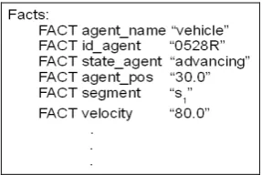
The agent behaviour (behavioural data generated by the agent) is determined by four interactive components. The first one, called facts, represents attributes and parameters describing drivers personality, namely preferred velocity, acceleration rate, etc. (see fig 4); the second component represents the agent activities, i.e. the tasks that change the agent state (stop, change lane, walk, etc.); the third one represents agent desires (goals and objectives); the fourth component is a decision making mechanism (DMM) allowing the agent to choice among alternative activities. DMM allows generating plans to reach agent goals using only agent activities in an intelligent way (rational agent).
[image:3.595.355.499.655.751.2]The agent activities are tasks that the agent can execute. Each type of agent has its own set of tasks. For instance, the set of tasks of vehicle is: advance, stop, accelerate, decelerate, change lane, and solve conflict. If an agent activity is executed then the agent state is changed, this statement is represented by changing some fact values. For instance accelerate increase the fact “velocity” in a 10%.
The agent desires are objectives or goals of the agent to modify their own state. For instance, “arrive to segment eight”.
The agent DMM cycle can be described as: Get a plan and execute the plan, specifically the steps are:
1. Get a plan. In order to compute a plan the agent desires and the environment information are used. The plan is a sequence of segments to be visited in order to reach the goal.
2. Decompose the plan into road user activities. In order to decompose the plan into agent activities, it is reactive response to the presence of other agents; first the agent must verify the environment state in a limited FOV, using a shared event list structure. Additionally one must take into account its own state. Afterwards a planning algorithm is executed [15] to translate the plan into a sequence of activities (a more detailed plan).
The evolving rules and traffic policies are taken in account when the DMM cycle is executed.
IV. MODELING UTSCOMPONENTS USING NLNS
The UTS model is expressed with n-LNS using three levels. In the first level the road network is described, the general behaviour of the road users is specified by level 2 nets; then the tasks or procedures needed to implement specific behaviours of the road user are represented by nets of level 3. A. First Level: The road network
The road network model can be straightforward obtained. For every segment si ∈S, a place pi is assigned. Then one transition tij is added for every (si, sj) in NC or NS, together with arcs (pi, tij) and (tij, pj). Furthermore some transitions ti must be added for every segment si source or sink; arcs (ti, pi) or (pi, ti) are added accordingly.
[image:4.595.328.523.52.238.2]Using this strategy the resulting model typeNet1,1 for the traffic network showed in fig. 5 is that showed in fig. 6. In table 1 are summarized other elements of this model; the static traffic signals for instance speed limit, bumps position, segment size, are information sent to the agent when a leavSeg transition is fired (t06, t17,etc.).
Fig. 5: Road Network
Fig. 6: Environment Net
Table 1: λ,τ and π functions of the net type typeNet1,1 typeNet1,1
TOKEN1 = { typeNet2,1} LABEL1 = {leavSeg, begChLn}
VAR1,1 = {x : typeNet2,1}
λ
λ{t01}=λ{t10}=λ{t67}=λ{t76}=λ{t34}=λ{t43}={(begChLn,↓)},λ{t06}=λ {t17}=λ{t62}=λ{t57}=λ{t63}=λ{t74}={(leavSeg,↓)}
τ
τ(p1) = τ(p2) =...= τ(pn) = {typeNet2,1} n is the number of segments
π
π((p0,t01),begChLn↓)= π((p1,t10),begChLn↓)= π((p6,t67),begChLn↓)=
π((p7,t76),begChLn↓)= π((p3,t34),begChLn↓)= π((p4,t43),begChLn↓)=
π((p0,t06),leavSeg↓)= π((p1,t17),leavSeg↓)= π((p6,t63),leavSeg↓)=
π((p7,t74),leavSeg↓)= π((p6,t62),leavSeg↓)= π((p5,t57),leavSeg↓)= x
B. Second Level: Agents
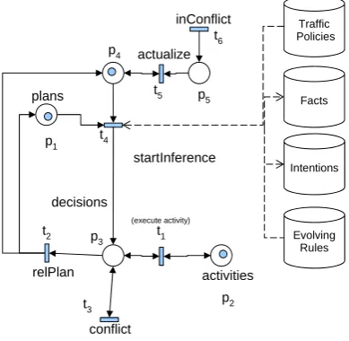
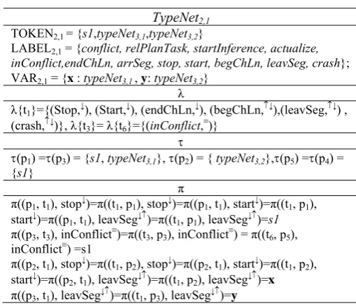
The decision making mechanism (DMM) of an agent is described by the net typeNet2,1showed in figure 7. During the reasoning process, the evolving rules and traffic policies are taken into account. In table 2 the elements of typeNet2,1are presented.
startInference plans
activities actualize
conflict
inConflict Traffic
Policies
Facts
Intentions
Evolving Rules
decisions
relPlan
t1
(execute activity)
t2
t3 t4
t5
t6
p1
p4
p5
[image:4.595.329.524.557.747.2]p2 p3
[image:4.595.87.259.632.757.2]Table 2: λ,τ and π functions of the net type typeNet2,1 TypeNet2,1
TOKEN2,1 = {s1,typeNet3,1,typeNet3,2}
LABEL2,1 = {conflict, relPlanTask, startInference, actualize,
inConflict,endChLn, arrSeg, stop, start, begChLn, leavSeg, crash}; VAR2,1 = {x : typeNet3,1, y: typeNet3,2}
λ
λ{t1}={(Stop,↓), (Start,↓), (endChLn,↓), (begChLn,↑↓),(leavSeg,↑↓) ,
(crash,↑↓)}, λ{t
3}= λ{t6}={(inConflict,≡)} τ
τ(p1) =τ(p3) = {s1, typeNet3,1}, τ(p2) = { typeNet3,2},τ(p5) =τ(p4) =
{s1}
π
π((p1, t1), stop↓)=π((t1, p1), stop↓)=π((p1, t1), start↓)=π((t1, p1),
start↓)=π((p
1, t1), leavSeg↓↑)=π((t1, p1), leavSeg↓↑)=s1 π((p3, t3), inConflict≡)=π((t3, p3), inConflict≡) = π((t6, p5),
inConflict≡) =s1
π((p2, t1), stop↓)=π((t1, p2), stop↓)=π((p2, t1), start↓)=π((t1, p2),
start↓)=π((p
2, t1), leavSeg↓↑)=π((t1, p2), leavSeg↓↑)=x π((p3, t1), leavSeg↓↑)=π((t1, p3), leavSeg↓↑)=y
The timing of traffic light (cycle time, green time of phases) is determined using traffic flow data of the road junction.
The resource conflict situation generated when an agent tries to execute one action that violate one evolving rule is captured in the model through the transitions actualize, inConflict, and conflict. It works as follows: the vehicle i decides execute a change lane event, and then it detects that the ubiquity E-Rule is violated. However, it decides execute the selected action (certain grade of irresponsibility or negligence). Nevertheless, before fire the negligence E-Rule, it is sent a message through the outConflict transition to the vehicle j in conflict. The vehicle j receives the message through the transition inConflict, then the actualize transition fires; this allows that the vehicle j actualizes its state when the vehicle i executes the change lane event. Then vehicle j initiates a reasoning process (startInference transition is fired) to make a decision about this event: either stop or crash (negligence E-Rule).
C. Third Level: Objects
Agent activities can be described by a third level net. In fig. 8 shows the typeNet3,1 that describe the vehicle driver activities and its possible states. If a in typeNet3,1 transition is fired, then a fact is modified.
leavSeg,arrSeg, begChLn, endChLn
stopped
advancing Fired Transitions
Position
endChLn,stop,leavSeg, Velocity
arrSeg Segment
leavSeg Mood
Stop Users
Modified Facts
endChLn, arrSeg, stop, leavSeg
t3 start
t1
crash, stop t2
p1
[image:5.595.307.565.97.274.2]p2
Fig. 8: Vehicle Activities Described by typeNet3,1 Each transition (agent event) modifies some of the agent facts; for instance the endChLn transition modifies the fact position. These events start a DMM cycle. For other
dynamical entities in the UTS, the behavior can be also represented by level 3 nets. The definition of the elements of typeNet3,1 is presented in table 3.
Table 3: λ,τ and π functions of the typeNet3,1 TypeNet3,1
TOKEN3,1 = {s1}; LABEL3,1 = {endChLn, arrSeg, stop, start,
begChLn, leavSeg,crash};VAR3,1 = {0} λ
λ{t3}={(endChLn,↑), (arrSeg,↑), (begChLn,↑), (leavSeg,↑)}, λ{t1}={(start,↑)}, λ{t2}={(stop,↑), (crash,↑)}
τ τ(p1) = τ(p2) ={s1}
π
π((p1, t1), start↑)=π((t1, p2), start↑)=π(( p2, t2), stop↑)=π(( t2, p1),
stop↑)=π(( p2, t2), crash↑)=π(( t2, p1), crash↑)= π((p2, t3),
endChLn↑)=π((t3, p2), endChLn↑)= π((p2, t3), arrSeg↑)=π((t3,
p2),arrSeg↑)=π((p2, t3),begChLn↑)=π((t3, p2), begChLn↑)=π((p2,
t3),leavSeg↑)=π((t3, p2), leavSeg↑)=s1
V. CONCLUSIONS
In this paper a UTS behavior model based in nLNS is presented. With the proposed modeling methodology hierarchical and modular UTS descriptions are built, adding clarity to the derived models. In this approach the road users are represented by mobile agents that evolve concurrently, allowing capturing more realistic UTS behavior. In the context of multi-agent systems, the present work contributes to the development of a more general modeling methodology to capture the environment rules, topological, geographical and dynamic UTS information. The proposed modeling methodology allows selecting the required level of microscopic road user’s behavior information. An important characteristic is the inclusion of the field of view concept which allows through the future event list analyzes the events of the neighbor agents and their environment state. A simulator is implemented using the resulted model; work is being done with regard to a distributed and parallel algorithm to execute the model.
REFERENCES
[1] J. Barcelo,“Microscopic Traffic Simulation: A tool for the analysis and assessment of ITS systems,” in Proc. of the Half Year Meeting of the Highway Capacity Committee, Lake Tahoe, 2001.
[2] J. Barceló, J. Ferrer, D., García, and R. Grau, “Microscopic Traffic simulation for ATT systems analysis. A parallel Computing version,” Contribution to the 25th anniversary of CRT, University of Montreal.
See (www.tss-bcn.com/documents.html).
[3] A. Cicortas, and N. Somosi, “Multi-Agent System Model for Urban Traffic Simulation,” in SACI '05: 2nd Romanian-Hungarian Joint
Symposium on Applied Computational Intelligence, May 12-14, 2005.
[4] L. Correia, and T. Wehrle, “Beyond cellular automata, towards more realistic traffic simulators,” in Cellular Automata - 7th International
Conference on Cellular Automata for Research and Industry ACRI 2006, Perpginan, France, September 2006, Proceedings, volume LNCS 4173, pp. 690-693. Springer.
[5] A. Di-Febraro, D. Giglio, and N. Sacco, “Modular Representation of Urban Traffic Systems based on Hybrid Petri nets,” in IEEE Intelligent Transportation Systems Conference proceedings. Oakland, 2001.
[image:5.595.49.284.606.716.2][7] F. Di-Cesare,P. Kulp, and M. Gile, “The application of Petri nets to the modeling, analysis and control of intelligent urban traffic networks,” 1994, En Proc. 15th Int. Conf. Application Theory Petri Nets, R. Valette, Ed. Zaragoza, Spain, pp. 2-15
[8] E. S. Hadouaj, A. Drogoul, and S. Espié; “A Multi-agent Road Traffic Simulation Model: Validation of the Insertion Case,” in Proceedings of 2004 Summer Computer Simulation Conference (SCSC’04), San Jose, California, USA; Juillet 2004.
[9] R. Jayakrishnan, C.E. Cortés, R. Lavanya and L. Pagès, “Simulation of Urban Transportation Networks with Multiple Vehicle Classes and Services: Classifications, Functional Requirements and General-Purpose Modelling Schemes,” in Proceedings of the 82th
Transportation Research Board Annual Meeting, Washington D.C., 2003.
[10] J. K. Lee, Y. H. Lim, and S. D. Chi, “Hierarchical modeling and simulation environment for intelligent transportation systems,” in Transactions of the Society for Computer Simulation International Simulation, Vol. 80, No. 2. (1 February 2004), pp. 61-76.
[11] R. Sánchez-Herrera, and E. López-Mellado, “Modular and Hierarchical Modeling of Interactive Mobile Agents,” in IEEE International Conference on Systems, Man and Cybernetics, Vol. 2, 10-13. pp. 1740-1745 vol.2. (2004)
[12] T. Schulze, T. Fliess, “Urban Traffic Simulation with psycho-physical vehicle/following models,” In Proceedings of the 1997 Winter Simulation Conference.
[13] R. Valk, “Petri Nets as Token Objets. An introduction to Elementary Object Nets,” in Int. Conf. on application and theory of Petri nets, pp:1-25, Springer-Verlag (1998)
[14] G. Wainer, N. Giambasi, "Specification, modelling and simulation of timed Cell-DEVS models," Technical Report 97-007, Departamento de computation, FCEN/UBA.
[15] M. Weerdt, A. Mors and C. Witteveen, “Multi-agent Planning: An introduction to planning and coordination” in Handouts of the European Agent Summer School, 2005, pp. 1-32
[16] D. Weyns, A. Omicini, and J. Odell, “Environment as a first class abstraction in multiagent systems,” in Autonomous Agents and Multi-Agent Systems, 2007,vol: 14, no. 1, pp.: 5–30.
[17] M. Wood, and S. DeLoach, “An overview of the multiagent systems engineering methodology,” In Proc. of the 1st Int. Workshop on Agent-Oriented Software Engineering, AOSE'00, pages 207--222, Limerick, Ireland, 2001.