Proceedings of the 2011 Conference on Empirical Methods in Natural Language Processing, pages 1092–1103, Edinburgh, Scotland, UK, July 27–31, 2011. c2011 Association for Computational Linguistics
Learning General Connotation of Words using Graph-based Algorithms
Song Feng Ritwik Bose Yejin Choi Department of Computer Science
Stony Brook University NY 11794, USA
songfeng, rbose, [email protected]
Abstract
In this paper, we introduce aconnotation lex-icon, a new type of lexicon that lists words with connotative polarity, i.e., words with pos-itive connotation (e.g., award, promotion) and words with negative connotation (e.g., cancer, war). Connotation lexicons differ from much studied sentiment lexicons: the latter concerns words thatexpresssentiment, while the former concerns words thatevoke or associate with a specific polarity of sentiment. Understand-ing the connotation of words would seem to require common sense and world knowledge. However, we demonstrate that much of the connotative polarity of words can be inferred from natural language text in a nearly unsu-pervised manner. The key linguistic insight behind our approach isselectional preference ofconnotative predicates. We present graph-based algorithms using PageRank and HITS that collectively learn connotation lexicon to-gether with connotative predicates. Our em-pirical study demonstrates that the resulting connotation lexicon is of great value for sen-timent analysis complementing existing senti-ment lexicons.
1 Introduction
In this paper, we introduce aconnotation lexicon, a new type of lexicon that lists words with conno-tative polarity, i.e., words with positive connotation (e.g., award, promotion) and words with negative connotation (e.g., cancer, war). Connotation lexi-cons differ from sentiment lexilexi-cons that are studied in much of previous research (e.g., Esuli and
Sebas-tiani (2006), Wilson et al. (2005a)): the latter con-cerns words thatexpresssentiment either explicitly or implicitly, while the former concerns words that
evokeor even simplyassociate witha specific polar-ity of sentiment. To our knowledge, there has been no previous research that investigates polarized con-notation lexicons.
Understanding the connotation of words would seem to require common sense and world knowl-edge at first glance, which in turn might seem to re-quire human encoding of knowledge base. However, we demonstrate that much of the connotative polar-ity of words can be inferred from natural language text in a nearly unsupervised manner.
The key linguistic insight behind our approach is
selectional preferenceofconnotative predicates. We define a connotative predicate as a predicate that has selectional preference on the connotative polar-ity of some of its semantic arguments. For instance, in the case of the connotative predicate“prevent”, there is strong selectional preference on negative connotation with respect to the thematic role (se-mantic role) “THEME”. That is, statistically speak-ing, people tend to associate negative connotation with the THEME of“prevent”, e.g., “prevent can-cer”or“prevent war”, rather than positive conno-tation, e.g., “prevent promotion”. In other words, even though it is perfectly valid to use words with positive connotation in the THEME role of “pre-vent”, statistically more dominant connotative po-larity is negative. Similarly, the THEME of “con-gratulate”or“praise”has strong selectional prefer-ence on positive connotation.
accomplish, achieve, advance, advocate, admire, applaud, appreciate, compliment, congratulate, develop, desire, enhance, enjoy, improve, praise, promote, respect, save, support, win
Table 1: Positively Connotative Predicates w.r.t. THEME
alleviate, accuse, avert, avoid, cause, complain, condemn, criticize, detect, eliminate, eradicate, mitigate, overcome, prevent, prohibit, protest, re-frain, suffer, tolerate, withstand
Table 2: Negatively Connotative Predicates w.r.t. THEME
preference of connotative predicates is that of se-mantic prosody in corpus linguistics. Sese-mantic prosody describes how some of the seemingly neu-tral words (e.g., “cause”) can be perceived with pos-itive or negative polarity because they tend to col-locate with words with corresponding polarity (e.g., Sinclair (1991), Louw et al. (1993), Stubbs (1995), Stefanowitsch and Gries (2003)). In this work, we demonstrate that statistical approaches that exploit this very concept of semantic prosody can success-fully infer connotative polarity of words.
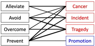
Having described the key linguistic insight, we now illustrate our graph-based algorithms. Figure 1 depicts the mutually reinforcing relation between connotative predicates (nodes on the left-hand side) and words with connotative polarity (node on the right-hand side). The thickness of edges represents the strength of the association between predicates and arguments. For brevity, we only consider conno-tation of words that appear in the THEMEthematic role.
We expect that words that appear often in the THEME role of various positively (or negatively) connotative predicates are likely to be words with positive (or negative) connotation. Likewise, pred-icates whose THEME contains words with mostly positive (or negative) connotation are likely to be positively (or negatively) connotative predicates. In short, we can induce the connotative polarity of words using connotative predicates, and inversely, we can learn new connotative predicates based on words with connotative polarity.
We hypothesize that this mutually reinforcing
re-Prevent Avoid
Alleviate Cancer
Incident
Promotion
Overcome Tragedy
Figure 1: Bipartite graph of connotative predicates and arguments. Edge weights are proportionate to the associ-ation strength.
lation between connotative predicates and their ar-guments can be captured via graph centrality in graph-based algorithms. Given a small set of seed words for connotative predicates, our algorithms collectively learn connotation lexicon together with connotative predicates in a nearly unsupervised manner. A number of different graph representa-tions are explored using both PageRank (Page et al., 1999) and HITS (Kleinberg, 1999) algorithms. Em-pirical study demonstrates that our graph based al-gorithms are highly effective in learning both con-notation lexicon and connotative predicates.
Finally, we quantify the practical value of our connotation lexicon in concrete sentiment analysis applications, and demonstrate that the connotation lexicon is of great value for sentiment classification tasks complementing conventional sentiment lexi-cons.
2 Connotation Lexicon & Connotative Predicate
In this section, we define connotation lexicon and
connotative predicates more formally, and contrast them against words in conventional sentiment lexi-cons.
2.1 Connotation Lexicon
This lexicon lists words with positive and negative connotation, as defined below.
• Words with positive connotation: In this
words with positive connotation. Some of these words may express subjectivity either explic-itly or implicexplic-itly, e.g., “joy” or “satisfaction”. However, a substantial number of words with positive connotation are purely objective, such as “life”, “health”, “tenure”, or “scientific”.
• Words with negative connotation:We define words with negative connotation as those that describe physical objects or abstract concepts that people generally disvalue or avoid. Sim-ilarly as before, some of these words may ex-press subjectivity (e.g., “disappointment”, “hu-miliation”), while many other are purely objec-tive (e.g., “bedbug”, “arthritis, “funeral”).
Note that this explicit and intentional inclusion of objective terms makes connotation lexicons differ from sentiment lexicons: most conventional senti-ment lexicons have focused on subjective words by definition (e.g., Wilson et al. (2005b)), as many re-searchers use the termsentimentandsubjectivity in-terchangeably (e.g., Wiebe et al. (2005)).
2.2 Connotative Predicate
In this work, connotative predicates are those that exhibit selectional preference on the connotative po-larity of some of their arguments. We emphasize that the polarity of connotative predicates doesnot coin-cide with the polarity of sentiment in conventional sentiment lexicons, as will be elaborated below.
• Positively connotative predicate: In this
work, we define positively connotative predi-cates as those that expect positive connotation in some arguments. For example, “congratu-late” or “save” are positively connotative pred-icates that expect words with positive conno-tation in the THEME argument: people typi-cally congratulate something positive, and save something people care about. More examples are shown in Table 1.
• Negatively connotative predicate: In this work, we define negatively connotative predi-cates as those that expect negative connotation in some arguments. For instance, predicates such as “prevent” or “suffer” tend to project negative connotation in the THEME argument. More examples are shown in Table 2.
Note that positively connotative predicates are not necessarily positive sentiment words. For instance “save” is not a positive sentiment word in the lexicon published by Wilson et al. (2005b). In-versely, (strongly) positive sentiment words are not necessarily (strongly) positively connotative predi-cates, e.g., “illuminate”, “agree”. Likewise, neg-atively connotative predicates are not necessarily negative sentiment words. For instance, predicates such as “prevent”, “detect”, or “cause” are not negative sentiment words, but they tend to corre-late with negative connotation in the THEME argu-ment. Inversely, (strongly) negative sentiment words are not necessarily (strongly) negatively connotative predicates, e.g., “abandon” (“abandoned [something valuable]”).
3 Graph Representation
In this section, we explore the graphical representa-tion of our task. Figure 1 depicts the key intuirepresenta-tion as a bipartite graph, where the nodes on the left-hand side correspond to connotative predicates, and the nodes on the right-hand side correspond to words in the THEME argument. There is an edge between a predicate p and an argument a, if the argument a appears in the THEMErole of the predicate p. For brevity, we explore only verbs as the predicates, and words in the THEMErole of the predicates as argu-ments. Our work can be readily extended to exploit other predicate-argument relations however.
Note that there are many sources of noise in the construction of graph. For instance, some of the predicates might be negated, changing the semantic dynamics between the predicate and the argument. In addition, there might be many unusual combina-tions of predicates and arguments, either due to data processing errors or due to idiosyncratic use of lan-guage. Some of such combinations can be valid ones (e.g., “prevent promotion”), challenging the learning algorithm with confusing evidence.
we next explore the directionality of the edges and different strategies to assign weights to them.
3.1 Undirected (Symmetric) Graph
First we explore undirected edges. In this case, we assign weight for each undirected edge between a predicate p and an argument a. Intuitively, the weight should correspond to the strength of relat-edness or association between the predicate p and the argument a. We use Pointwise Mutual Infor-mation (PMI), as it has been used by many pre-vious research to quantify the association between two words (e.g., Turney (2001), Church and Hanks (1990)). The PMI score betweenpandais defined as follows:
w(p−a) :=P M I(p, a) =log P(p, a) P(p)P(a)
The log of the ratio is positive when the pair of words tends to co-occur and negative when the pres-ence of one word correlates with the abspres-ence of the other word.
3.2 Directed (Asymmetric) Graph
Next we explore directed edges. That is, for each connected pair of a predicatep and an argumenta, there are two edges in opposite directions:e(p→a) and e(a → p). In this case, we explore the use of asymmetric weights using conditional probabil-ity. In particular, we define weights as follows:
w(p→a) :=P(a|p) = P(p, a) P(p)
w(a→p) :=P(p|a) = P(p, a) P(a)
Having defined the graph structure, next we explore algorithms that analyze graph centrality via random walks. In particular, we investigate the use of HITS algorithm (Section 4), and PageRank (Section 5).
4 Lexicon Induction using HITS
The graph representation described thus far (Sec-tion 3) captures general semantic rela(Sec-tions between predicates and arguments, rather than those specific to connotative predicates and arguments. Therefore in this section, we explore techniques to augment the graph representation so as to bias the centrality
of the graph toward connotative predicates and argu-ments.
In order to establish a learning bias, we start with a small set of seed words forjustconnotative predi-cates. We use 20 words for each polarity, as listed in Table 1 and Table 2. These seed words act as prior knowledge in our learning. We explore two different techniques to incorporate prior knowledge into ran-dom walk, as will be elaborated in Section 4.2 & 4.3, followed by brief description of HITS in Section 4.1.
4.1 Hyperlink-Induced Topic Search (HITS) HITS (Hyperlink-Induced Topic Search) algorithm (Kleinberg, 1999), also known as Hubs and author-ities, is a link analysis algorithm that is particularly suitable to model mutual reinforcement between two different types of nodes: hubs and authorities. The definitions of hubs and authorities are given recur-sively. A (good) hub is a node that points to many (good) authorities, and a (good) authority is a node pointed by many (good) hubs.
Notice that the mutually reinforcing relation-ship is precisely what we intend to model between connotative predicates and arguments. Let G = (P, A, E)be the bipartite graph, whereP is the set of nodes corresponding to connotative predicates,A is the set of nodes corresponding to arguments, and E is the set of edges among nodes. (Pi, Aj) ∈ E
if and only if the predicatePi and the argumentAi
occur together as a predicate – argument pair in the corpus. The co-occurrence matrix derived from our corpus is denoted asL, where
Lij =
(
w(i, j) if(Pi, Aj)∈E
0 otherwise
The value of w(i, j) is set to w(i−j) as defined in Section 3.1 for undirected graphs, andw(i→ j) defined in Section 3.2 for directed graphs.
Let a(Ai) and h(Ai) be the authority and hub
score respectively, for a given nodeAi ∈ A. Then
we compute the authority and hub score recursively as follows:
a(Ai) =
X
Pi,Aj∈E
w(i, j)h(Aj) +
X
Pj,Ai∈E
h(Pj)w(j, i)
h(Ai) =
X
Pi,Aj∈E
w(i, j)a(Aj) +
X
Pj,Ai∈E
a(Pj)w(j, i)
The scoresa(Pi)andh(Pi)forPi ∈ P are defined
similarly as above.
In what follows, we describe two different tech-niques to incorporate prior knowledge. Note that it is possible to apply each of the following techniques to both directed and undirected graph representa-tions introduced in Section 3. Also note that for each technique, we construct two separate graphsG+and G− corresponding to positive and negative polarity respectively. That is,G+ learns positively
connota-tive predicates and arguments, whileG−learns neg-atively connotative predicates and arguments.
4.2 Prior Knowledge via Truncated Graph First we introduce a method based on graph trunca-tion. In this method, when constructing the bipartite graph, we limit the set of predicatesP to only those words in the seed set, instead of including all words that can be predicates. In a way, the truncated graph representation can be viewed as the query induced graph on which the original HITS algorithm was in-vented (Kleinberg, 1999).
The truncated graph is very effective in reducing the level of noise that can be introduced by predi-cates of the opposite polarity. It may seem like we cannot discover new connotative predicates in the truncated graph however, as the graph structure is limited only to the seed predicates. We address this issue by alternating truncation to different side of the graph, i.e., left (predicates) or right (arguments), as illustrated in Figure 1, through multiple rounds of HITS.
For instance, we start with the graph G = (Po, A, E(Po)) that is truncated only on the left-hand side, with the seed predicatesPo. Here,E(Po)
denotes the reduced set of edges discarding those edges that connect to predicates not inPo. Then, we apply HITS algorithm until convergence to discover new words with connotation, and this completes the first round of HITS.
Next we begin the second round. Let Ao be the
new words with connotation that are found in the first round. We now set Ao as seed words for the second phase of HITS, where we construct a new graph G = (P, Ao, E(Ao)) that is truncated only on the right-hand side, with full candidate words for predicates included on the left-hand side. This al-ternation can be repeated multiple times to discover
many new connotative predicates and arguments.
4.3 Prior Knowledge via Focussed Graph In the truncated graph described above, one poten-tial concern is that the discovery of new words with connotation is limited to those that happen to corre-late well with the seed predicates. To mitigate this problem, we explore an alternative technique based on the full graph, which we will name as focussed graph.
In this method, instead of truncating the graph, we simply emphasize the important portion of the graph via edge weights. That is, we assign high weights to those edges that connect a seed predicate with an ar-gument, while assigning low weights for those edges that connect to a predicate outside the seed set. This way, we allow predicates not in the seed set to par-ticipate in hubs and authority scores, but in a much suppressed way. This method can be interpreted as a smoothed version of the truncated graph described in Section 4.2.
More formally, if the node Ai is connected to
the seed predicate Pj, the value of co-occurrence
matrix Lij is defined by prior knowledge(e.g.
P M I(Ai, Pj)orP(Ai|Pj)), otherwise a small
con-stantis assigned to the edge.
Lij =
(
w(i, j) if Pj ∈Eo
otherwise
Similarly to the truncated graph, we proceed with multiple rounds of HITS, focusing different part of the bipartite graph alternately.
5 Lexicon Induction using PageRank In this section, we explore the use of another popu-lar approach for link analysis: PageRank (Page et al., 1999). We first describe PageRank algorithm briefly in Section 5.1, then introduce two different techniques to incorporate prior knowledge in Sec-tion 5.2 and 5.3.
5.1 PageRank
Let G = (V, E) be the graph, where vi ∈ V =
P ∪A are nodes (words) for the disjunctive set of predicates (P) and arguments (A), ande(i,j) ∈ E are edges. Let In(i) be the set of nodes with an edge leading toni and similarly, Out(i) be the set
of nodes thatni has an edge leading to. At a given
iteration of the algorithm, we update the score ofni
as follows:
S(i) =α X
j∈In(i)
S(j)× w(i, j)
|Out(i)|+ (1−α) (1)
where the valueα is constantdamping factor. The value of α is typically set to 0.85. The value of w(i, j)is set tow(i−j)as defined in Section 3.1 for undirected graphs, andw(i→ j)as defined in Sec-tion 3.2 for directed graphs. As before, we will con-sider two different techniques to incorporate prior knowledge into the graph analysis as follows. 5.2 Prior Knowledge via Truncated Graph Unlike HITS, which was originally invented for a query-induced graph, PageRank is typically applied to the full graph. However, we can still apply the truncation technique introduced in Section 4.2 to PageRank as well. To do so, when constructing the bipartite graph, we limit the set of predicatesP to only those words in the seed set, instead of including all words that can be predicates. Graph truncation eliminates the noise that can be introduced by pred-icates of the opposite polarity. However, in order to learn new predicates, we need to perform multiple rounds of PageRank, truncating different side of the bipartite graph alternately. Refer to Section 4.2 for futher details.
5.3 Prior Knowledge via Teleportation
We next explore what is known as teleportation technique for topic sensitive PageRank (Haveliwala, 2002). For this, we use the following equation that is slightly augmented from Equation 1.
S(i) =α X
j∈In(i)
S(j)× w(i, j)
|Out(i)|+ (1−α)i (2)
Here, the new termiis asmoothing factorthat
pre-vents cliques in the graph from garnering reputation through feedback (Bianchini et al. (2005)). In or-der to emphasize important portion of the graph, i.e., subgraphs connected to the seed set, we assign non-zeroscores to only those important nodes, i.e., the seed set. Intuitively, this will cause the random walk to restart from the seed set with(1−α)= 0.15 prob-ability for each step.
6 The Use of Google Web 1T Data
In order to implement the network of connotative predicates and arguments, we need a substantially large amount of documents. The quality of the co-occurrence statistics is expected to be proportionate to the size of corpus, but collecting and process-ing such a large amount of data is not trivial. We therefore resort to the Google Web 1T data (Brants and Franz., 2006), which consists of Googlen-gram counts (frequency of occurrence of eachn-gram) for 1≤n≤5. The use of Web 1T data will lessen the challenge with respect to data acquisition, while still allowing us to enjoy the co-occurrence statistics of web-scale data. Because Web 1T data is justn-gram statistics, rather than a collection of normal docu-ments, it does not provide co-occurrence statistics of any random word pairs. However, it provides a nice approximation to the particular co-occurrence statis-tics we are interested in, which are, predicate – ar-gument pairs. This is because the THEMEargument of a verb predicate is typically on the right hand side of the predicate, and the argument is within the close range of the predicate.
We now describe how to derive co-occurrence statistics of each predicate – argument pair using the Web 1T data. For a given predicatepand an argu-menta, we add up the count (frequency) of all n -grams (2≤n≤5) that match the following pattern:
[p] [?]n−2[a]
wherepmust be the first word (head),amust be the last word (tail), and[?]n−2matches anyn−2 num-ber of words between pand a. Note that this rule enforces the argumentato be on the right hand side of the predicatep. To reduce the level of noise, we do not allow the wildcard[?]to match any punctu-ation mark, as such n-grams are likely to cross sen-tence boundaries representing invalid predicate – ar-gument relations. We consider a word as a predicate if it is tagged as a verb by a Part-of-Speech tagger (Toutanova and Manning, 2000). For argument[a], we only consider content-words.
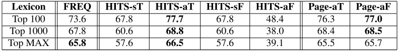
Lexicon FREQ HITS-sT HITS-aT HITS-sF HITS-aF Page-aT Page-aF
Top 100 73.6 67.8 77.7 67.8 48.4 76.3 77.0
Top 1000 67.8 60.6 68.8 60.6 38.0 68.4 68.5
[image:7.612.108.506.71.123.2]Top MAX 65.8 57.6 66.5 57.6 39.1 65.5 65.7
Table 3: Comparison Result with General Inquirer Lexicon(%)
Lexicon FREQ HITS-sT HITS-aT HITS-sF HITS-aF Page-aT Page-aF
Top 100 83.0 79.3 86.3 79.3 55.8 86.3 87.2
Top 1000 80.3 67.3 81.3 67.3 46.5 80.7 80.3 Top MAX 71.5 62.7 72.2 62.7 45.4 71.1 72.3
Table 4: Comparison Result with OpinionFinder (%)
PageRank — will be able to discern valid relations from noise, by focusing on the important part of the graph. In other words, we expect that good predi-cates will be supported by good arguments, and vice versa, thereby resulting in a reliable set of predicates and arguments that are mutually supported by each other.
7 Experiments
As a baseline, we use a simple method dubbed
FREQ, which uses co-occurrence frequency with respect to the seed predicates. Using the pattern [p] [?]n−2 [a] (see Section 6), we collect two sets of n-gram records: one set using the positive con-notative predicates, and the other using the negative connotative predicates. With respect to each set, we calculate the following for each worda,
• Given [a], the number of unique[p]asf1
• Given [a], the number of unique phrases[?]n−2 asf2
• The number of occurrences of[a]asf3
We then obtain the scoreσa+ for positive
connota-tion andσa−for negative connotation using the
fol-lowing equations that take a linear combination of f1,f2, andf3that we computed above with respect to each polarity.
σa+ =α×σf1++β×σf2++γ×σf3+ (3)
σa−=α×σf1−+β×σf2−+γ×σf3− (4)
Note that the coefficientsα,βandγare determined experimentally. We assign positive polarity to the worda, ifσa+ >> σa−and vice versa.
7.1 Comparison against Sentiment Lexicon The polarity defined in the connotation lexicon dif-fers from that of conventional sentiment lexicons in which we aim to recognize more subtle sentiment that correlates with words. Nevertheless, we provide agreement statistics between our connotation lexi-con and lexi-conventional sentiment lexilexi-cons for com-parison purposes. We collect statistics with respect to the following two resources: General Inquirer (Stone and Hunt, 1963) and Opinion Finder (Wilson et al., 2005b).
For polarityλ ∈ {+,−}, letcountsentlex(λ) denote the total number of words labeled as λ in a given sentiment lexicon, and let countagreement(λ) denote
the total number of words labeled asλby both the given sentiment lexicon and our connotation lexi-con. In addition, letcountoverlap(λ) denote the total
number of words that are labeled asλby our conno-tation lexicon that are also included in the reference lexicon with or without the same polarity. Then we computeprecλas follows:
precλ % =
countagreement(λ) countoverlap(λ) ×
100
We compareprecλ % for three different segments
of our lexicon: the top100, top1000, and the entire lexicon. We compare the lexicons provided by the seven variations of our algorithm. Results are shown in Table 3 & 4.
Positive: include, offer, obtain, allow, build, in-crease, ensure, contain, pursue, fulfill, maintain, recommend, represent, require, respect
Negative: abate, die, condemn, deduce, investi-gate, commit, correct, apologize, debilitate, dis-pel, endure, exacerbate, indicate, induce, mini-mize
Table 5: Examples of newly discovered connotative pred-icates
Positive: boogie, housewarming, persuasiveness, kickoff, playhouse, diploma, intuitively, monu-ment, inaugurate, troubleshooter, accompanist Negative: seasickness, overleap, gangrenous, suppressing, fetishist, unspeakably, doubter, bloodmobile, bureaucratized
Table 6: Examples of newly discovered words with notations: these words are treated as neutral in some con-ventional sentiment lexicons.
symmetric and asymmetric version of the Focused method. Finally,Page-aT&Page-aFcorrespond to the Truncation and teleportation (Focused) respec-tively.
Asymmetric HITS on a directed truncated graph (HITS-aT) and topic-sensitive PageRank (Page-aF) achieve the best performance in most cases, espe-cially for top ranked words which have a higher average frequency. The difference between these two top performers is not large, but statistically significant using wilcoxon test with p < 0.03. Standard PageRank (Page-aT) achieves the third best performance overall. All these top performing ones (HITS-aT,Page-aF,Page-aT) outperform the baseline approach (FREQ) statistically significantly withp <0.001. For brevity, we omit the PageRank results based on the undirected graphs, as the perfor-mance of those was not as good as that of directed ones.
7.2 Extrinsic Evaluation via Sentiment Analysis
Next we perform extrinsic evaluation to quantify the practical value of our connotation lexicon in con-crete sentiment analysis applications. In particular, we make use of our connotation lexicon for binary
sentiment classification tasks in two different ways:
• Unsupervised classification by voting. We de-finer as the ratio of positive polarity words to negative polarity words in the lexicon. In our experiment, penalty is0for positive and−0.5 for negative.
score(x+) = 1 +penalty+(r,#positive)
score(x−) =−1 +penalty−(r,#negative)
• Supervised classification using SVM. We use
bag-of-words features for baseline. In order to quantify the effect of different lexicons, we add additional features based on the following scores as defined below:
scoreraw(x) =
X
wx
s(w)
scorepurity(x) =
scoreraw(x)
P
wxabs(s(w))
The two corpora we use are SemEval2007 (Strap-parava and Mihalcea, 2007) and Sentiment Twitter.1 The Twitter dataset consists of tweets containing ei-ther asmiley emoticon (representing positive senti-ment) or afrowny emoticon (representing negative sentiment), we randomly select50000smileytweets and 50000 frowny tweets.2 We perform a 5-fold cross validation.
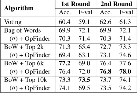
In Table 8, we find very promising results, partic-ularly for Twitter dataset, which is known to be very noisy. Notice that the use of Top 6k words from our connotation lexicon along with OpinionFinder lexicon boost the performance up to 78.0%, which is significantly better than than 71.4% using only the conventional OpinionFinder lexicon. This result shows that our connotation lexicon nicely comple-ments existing sentiment lexicon, improving practi-cal sentiment analysis tasks.
1http://www.stanford.edu/˜ alecmgo/cs224n/twitterdata.
2009.05.25.c.zip
2We filter out stop-words and words appearing less than 3
times. For Twitter, we also remove usernames of the format @usernameoccurring within tweet bodies.
Algorithm Acc. F-val Acc. F-val1st Round 2nd Round
Voting 68.7 65.4 71.0 68.5 Bag of Words 69.9 65.1 69.9 65.1 (00) + OpFinder 74.7 75.0 74.7 75.0
BoW + Top 2k 73.3 74.5 73.7 75.4 (00) + OpFinder 72.8 73.5 75.0 77.6 BoW + Top 6k 76.6 77.1 74.5 75.3 (00) + OpFinder 74.1 73.5 75.2 76.0
[image:9.612.74.299.71.225.2]BoW + Top 10k 74,1 73.5 74.2 73.8 (00) + OpFinder 73.5 74.3 74.7 75.1
Table 7: SemEval Classification Result(%) — (00) denotes that all features in the previous row are copied over.
Algorithm Acc. F-val Acc. F-val1st Round 2nd Round Voting 60.4 59.1 62.6 61.3 Bag of Words 69.9 72.1 69.9 72.1 (00) + OpFinder 70.3 71.4 70.3 71.4 BoW + Top 2k 71.3 65.4 72.7 73.3 (00) + OpFinder 69.4 63.1 73.1 74.6
BoW + Top 6k 77.2 69.0 76.4 77.6 (00) + OpFinder 76.4 72.0 76.8 78.0 BoW + Top 10k 73.3 73.5 73.7 74.1 (00) + OpFinder 74.1 69.5 73.5 74.2
Table 8: Twitter Classification Result(%) — (00) denotes that all features in the previous row are copied over.
7.3 Intrinsic Evaluation via Human Judgment In order to measure the quality of the connotation lexicon, we also perform human judgment study on a subset of the lexicon. Human judges are asked to quantify the degree of connotative polarity of each given word using an integer value between1and5, where1and5correspond to the most negative and positive connotation respectively. When computing the annotator agreement score or evaluating our notation lexicon against human judgment, we con-solidate 1 and 2 into a single negative class and 4 and 5 into a single positive class. The Kappa score between two human annotators is 0.78.
As a control set, we also include100words taken from the General Inquirer lexicon: 50 words with positive sentiment, and50words with negative sen-timent. These words are included so as to
mea-sure the quality of human judgment against a well-established sentiment lexicon. The words were pre-sented in a random order so that the human judges will not know which words are from the General In-quirer lexicon and which are from our connotative lexicon. For the words in the control set, the anno-tators achieved 94% (97% lenient) accuracy on the positive set and 97% on the negative set.
Note that some words appear in both positive and negative connotation graphs, while others appear in only one of them. For instance, if a given word x appears as an argument for only positive connotative predicates, but never for negative ones, thenxwould appear only in the positive connotation graph. This means that for such word, we can assume the conno-tative polarity even without applying the algorithms for graph centrality. Therefore, we first evaluate the accuracy of the polarity of such words that appear only in one of the connotation graphs. We discard words with low frequency (300 in terms of Google n-gram frequency), and randomly select 50 words from each polarity. The accuracy of such words is 88% by strict evaluation and 94.5% by lenient eval-uation, where lenient evaluation counts words in our polarized connotation lexicon to be correct if the hu-man judges assign non-conflicting polarities, i.e., ei-ther neutral or identical polarity.
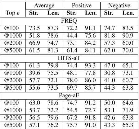
For words that appear in both positive and nega-tive connotation graphs, we determine the final po-larity of such words as one with higher scores given by HITS or PageRank. We randomly select words that rank at 5% of top 100, top 1000, top 2000, and top 5000 by each algorithm for human judgment. We only evaluate the top performing algorithms – HITS-aT and Page-aF – and FREQ baseline. The stratified performance for each of these methods is given in Table 9.
8 Related Work
[image:9.612.73.299.275.428.2]Average Positive Negative Top # Str. Len. Str. Len. Str. Len.
FREQ
@100 73.5 87.3 72.2 91.1 74.7 83.5 @1000 51.8 78.6 44.4 75.6 81.8 90.9 @2000 66.9 74.7 73.1 84.2 57.3 60.0 @5000 61.5 81.3 61.4 84.1 62.0 70.0
HITS-aT
@100 61.3 79.8 74.4 93.3 47.0 65.1 @1000 39.6 75.5 48.1 77.8 30.8 73.1 @2000 57.7 72.1 78.0 86.0 41.0 60.7 @5000 55.6 73.5 69.7 85.7 44.3 63.8
Page-aF
[image:10.612.72.296.69.277.2]@100 63.0 78.6 74.7 91.2 50.0 64.6 @1000 53.7 72.2 54.5 72.7 53.1 71.9 @2000 56.5 79.6 67.2 91.8 42.6 63.8 @5000 57.1 76.2 75.7 91.0 43.3 65.3
Table 9: Human Annotation Accuracies(%) – Str. de-notes strict evaluation &Len.denotes lenient evaluation.
present systematic comparison of various options for graph representation and encoding of prior knowl-edge. We are not aware of any previous research that made use of HITS algorithm for connotation or sentiment lexicon induction.
Much of previous research investigated the use of dictionary network (e.g., WordNet) for lexicon in-duction (e.g., Kamps et al. (2004), Takamura et al. (2005), Adreevskaia and Bergler (2006), Esuli and Sebastiani (2006), Su and Markert (2009), Moham-mad et al. (2009)), while relatively less research in-vestigated the use of web documents (e.g., Kaji and Kitsuregawa (2007), Velikovich et al. (2010))).
Wilson et al. (2005b) first introduced the sen-timent lexicon, spawning a great deal of research thereafter. At the beginning, sentiment lexicons were designed to include only those words that ex-presssentiment, that is,subjectivewords. However in recent years, sentiment lexicons started expand-ing to include some of those words that simply asso-ciate with sentiment, even if those words are purely objective (e.g., Velikovich et al. (2010), Baccianella et al. (2010)). This trend applies even to the most re-cent version of the lexicon of Wilson et al. (2005b). We conjecture that this trend of broader coverage suggests that such lexicons are practically more use-ful than sentiment lexicons that include only those words that are strictly subjective. In this work, we
make this transition more explicit and intentional, by introducing a novelconnotation lexicon.
Mohammad and Turney (2010) focussed on emo-tion evoked by common words and phrases. The spirit of their work shares some similarity with ours in that it aims to find the emotionevokedby words, as opposed toexpressed. Two main differences are: (1) our work aims to discover even more subtle asso-ciation of words with sentiment, and (2) we present a nearly unsupervised approach, while Mohammad and Turney (2010) explored the use of Mechanical Turk to build the lexicon based on human judgment. In the work of Osgood et al. (1957), it has been discussed that connotative meaning of words can be measured in multiple scales of semantic differ-ential, for example, the degree of “goodness” and “badness”. Our work presents statistical approaches that measure one such semantic differential auto-matically. Our graph construction to capture word-to-word relation is analogous to that of Collins-Thompson and Callan (2007), where the graph rep-resentation was used to model more general defini-tions of words.
9 Conclusion
We introduced theconnotation lexicon, a novel lex-icon that list words with connotative polarity, which will be made publically available. We also pre-sented graph-based algorithms for learning conno-tation lexicon together with connotative predicates in a nearly unsupervised manner. Our approaches are grounded on the linguistic insight with respect to the selectional preference of connotative predicates. Empirical study demonstrates the practical value of the connotation lexicon for sentiment analysis en-couraging further research in this direction.
Acknowledgments
We wholeheartedly thank the reviewers for very helpful and insightful comments.
References
Alina Adreevskaia and Sabine Bergler. 2006. Mining wordnet for fuzzy sentiment: Sentiment tag extraction from wordnet glosses. In11th Conference of the Eu-ropean Chapter of the Association for Computational Linguistics, pages 209–216.
Stefano Baccianella, Andrea Esuli, and Fabrizio Se-bastiani. 2010. Sentiwordnet 3.0: An enhanced lexical resource for sentiment analysis and opinion mining. In Nicoletta Calzolari (Conference Chair), Khalid Choukri, Bente Maegaard, Joseph Mariani, Jan Odijk, Stelios Piperidis, Mike Rosner, and Daniel Tapias, editors,Proceedings of the Seventh conference on International Language Resources and Evaluation (LREC’10), Valletta, Malta, may. European Language Resources Association (ELRA).
Monica Bianchini, Marco Gori, and Franco Scarselli. 2005. Inside pagerank.ACM Trans. Internet Technol., 5:92–128, February.
Thorsten Brants and Alex Franz. 2006. Web 1t 5-gram version 1. In Linguistic Data Consortium, ISBN: 1-58563-397-6, Philadelphia.
Kenneth Ward Church and Patrick Hanks. 1990. Word association norms, mutual information, and lexicogra-phy. Comput. Linguist., 16:22–29, March.
K. Collins-Thompson and J. Callan. 2007. Automatic and human scoring of word definition responses. In Proceedings of NAACL HLT, pages 476–483.
Andrea Esuli and Fabrizio Sebastiani. 2006. Sentiword-net: A publicly available lexical resource for opinion mining. InIn Proceedings of the 5th Conference on Language Resources and Evaluation (LREC06, pages 417–422.
Andrea Esuli and Fabrizio Sebastiani. 2007. Pagerank-ing wordnet synsets: An application to opinion min-ing. InProceedings of the 45th Annual Meeting of the Association of Computational Linguistics, pages 424– 431. Association for Computational Linguistics. Taher H. Haveliwala. 2002. Topic-sensitive pagerank. In
Proceedings of the Eleventh International World Wide Web Conference, Honolulu, Hawaii.
Nobuhiro Kaji and Masaru Kitsuregawa. 2007. Build-ing lexicon for sentiment analysis from massive collec-tion of HTML documents. InProceedings of the Joint Conference on Empirical Methods in Natural guage Processing and Computational Natural Lan-guage Learning (EMNLP-CoNLL), pages 1075–1083. Jaap Kamps, Maarten Marx, Robert J. Mokken, and Maarten De Rijke. 2004. Using wordnet to mea-sure semantic orientation of adjectives. In Proceed-ings of the 4th International Conference on Language Resources and Evaluation (LREC), pages 1115–1118. Jon M. Kleinberg. 1999. Authoritative sources in a hy-perlinked environment. JOURNAL OF THE ACM, 46(5):604–632.
B. Louw, M. Baker, G. Francis, and E. Tognini-Bonelli. 1993. Irony in the text or insincerity in the writer? the diagnostic potential of semantic prosodies. TEXT AND TECHNOLOGY IN HONOUR OF JOHN SIN-CLAIR, pages 157–176.
Saif Mohammad and Peter Turney. 2010. Emotions evoked by common words and phrases: Using me-chanical turk to create an emotion lexicon. In Pro-ceedings of the NAACL HLT 2010 Workshop on Com-putational Approaches to Analysis and Generation of Emotion in Text, pages 26–34, Los Angeles, CA, June. Association for Computational Linguistics.
Saif Mohammad, Cody Dunne, and Bonnie Dorr. 2009. Generating high-coverage semantic orientation lexi-cons from overtly marked words and a thesaurus. In Proceedings of the 2009 Conference on Empiri-cal Methods in Natural Language Processing, pages 599–608, Singapore, August. Association for Compu-tational Linguistics.
C. E. Osgood, G. Suci, and P. Tannenbaum. 1957. The measurement of meaning. University of Illinois Press, Urbana, IL.
Lawrence Page, Sergey Brin, Rajeev Motwani, and Terry Winograd. 1999. The pagerank citation ranking: Bringing order to the web. Technical Report 1999-66, Stanford InfoLab, November.
Delip Rao and Deepak Ravichandran. 2009. Semi-supervised polarity lexicon induction. In EACL ’09: Proceedings of the 12th Conference of the European Chapter of the Association for Computational Linguis-tics, pages 675–682, Morristown, NJ, USA. Associa-tion for ComputaAssocia-tional Linguistics.
John Sinclair. 1991. Corpus, concordance, colloca-tion. Describing English language. Oxford University Press.
A. Stefanowitsch and S.T. Gries. 2003. Collostructions: Investigating the interaction of words and construc-tions. International Journal of Corpus Linguistics, 8(2):209–243.
Philip J. Stone and Earl B. Hunt. 1963. A computer ap-proach to content analysis: studies using the general inquirer system. In Proceedings of the May 21-23, 1963, spring joint computer conference, AFIPS ’63 (Spring), pages 241–256, New York, NY, USA. ACM. Carlo Strapparava and Rada Mihalcea. 2007. Semeval-2007 task 14: affective text. In SemEval ’07: Pro-ceedings of the 4th International Workshop on Seman-tic Evaluations, pages 70–74, Morristown, NJ, USA. Association for Computational Linguistics.
M. Stubbs. 1995. Collocations and semantic profiles: on the cause of the trouble with quantitative studies. Functions of language, 2(1):23–55.
Fangzhong Su and Katja Markert. 2009. Subjectivity recognition on word senses via semi-supervised min-cuts. InProceedings of Human Language Technolo-gies: The 2009 Annual Conference of the North Amer-ican Chapter of the Association for Computational Linguistics, pages 1–9. Association for Computational Linguistics.
Hiroya Takamura, Takashi Inui, and Manabu Okumura. 2005. Extracting semantic orientations of words using spin model. InProceedings of ACL-05, 43rd Annual Meeting of the Association for Computational Linguis-tics, Ann Arbor, US. Association for Computational Linguistics.
Kristina Toutanova and Christopher D. Manning. 2000. Enriching the knowledge sources used in a maximum entropy part-of-speech tagger. In In EMNLP/VLC 2000, pages 63–70.
Peter Turney. 2001. Mining the web for synonyms: Pmi-ir versus lsa on toefl.
Leonid Velikovich, Sasha Blair-Goldensohn, Kerry Han-nan, and Ryan McDonald. 2010. The viability of web-derived polarity lexicons. InHuman Language Tech-nologies: The 2010 Annual Conference of the North American Chapter of the Association for Computa-tional Linguistics. Association for Computational Lin-guistics.
Janyce Wiebe, Theresa Wilson, and Claire Cardie. 2005. Annotating expressions of opinions and emotions in language. Language Resources and Evaluation (for-merly Computers and the Humanities), 39(2/3):164– 210.
Theresa Wilson, Paul Hoffmann, Swapna Somasun-daran, Jason Kessler, Janyce Wiebe, Yejin Choi, Claire Cardie, Ellen Riloff, and Siddharth Patwardhan. 2005a. Opinionfinder: a system for subjectivity anal-ysis. In Proceedings of HLT/EMNLP on Interactive Demonstrations, pages 34–35, Morristown, NJ, USA. Association for Computational Linguistics.
Theresa Wilson, Janyce Wiebe, and Paul Hoffmann. 2005b. Recognizing contextual polarity in phrase-level sentiment analysis. InHLT ’05: Proceedings of the conference on Human Language Technology and Empirical Methods in Natural Language Processing, pages 347–354, Morristown, NJ, USA. Association for Computational Linguistics.
Xiaojin Zhu and Zoubin Ghahramani. 2002. Learn-ing from labeled and unlabeled data with label prop-agation. In Technical Report CMU-CALD-02-107. CarnegieMellon University.