A Semi Supervised Approach to Improve Classification of Infrequent Discourse Relations Using Feature Vector Extension

A Semi-Supervised Approach to Improve Classification of

Infrequent Discourse Relations using Feature Vector Extension

Hugo Hernault [email protected]. u-tokyo.ac.jp

Danushka Bollegala [email protected].

u-tokyo.ac.jp

Graduate School of Information Science & Technology The University of Tokyo

7-3-1 Hongo, Bunkyo-ku, Tokyo 113-8656, Japan

Mitsuru Ishizuka ishizuka@i. u-tokyo.ac.jp

Abstract

Several recent discourse parsers have em-ployed fully-supervised machine learning ap-proaches. These methods require human an-notators to beforehand create an extensive training corpus, which is a time-consuming and costly process. On the other hand, un-labeled data is abundant and cheap to col-lect. In this paper, we propose a novel semi-supervised method for discourse rela-tion classificarela-tion based on the analysis of co-occurring features in unlabeled data, which is then taken into account for extending the fea-ture vectors given to a classifier. Our exper-imental results on the RST Discourse Tree-bank corpus and Penn Discourse TreeTree-bank in-dicate that the proposed method brings a sig-nificant improvement in classification accu-racy and macro-average F-score when small training datasets are used. For instance, with training sets of c.a.1000labeled instances, the proposed method brings improvements in ac-curacy and macro-average F-score up to50%

compared to a baseline classifier. We believe that the proposed method is a first step towards detecting low-occurrence relations, which is useful for domains with a lack of annotated data.

1 Introduction

Automatic detection of discourse relations in natu-ral language text is important for numerous tasks in NLP, such as sentiment analysis (Somasundaran et al., 2009), text summarization (Marcu, 2000) and di-alogue generation (Piwek et al., 2007). However, most of the recent work employing discourse re-lation classifiers are based on fully-supervised ma-chine learning approaches (duVerle and Prendinger,

2009; Pitler et al., 2009; Lin et al., 2009). Two of the main corpora with discourse annotations are the RST Discourse Treebank (RSTDT) (Carlson et al., 2001) and the Penn Discourse Treebank (PDTB) (Prasad et al., 2008a), which are both based on the Wall Street Journal (WSJ) corpus.

In the RSTDT, annotation is done using 78

fine-grained discourse relations, which are usually grouped into18 coarser-grained relations. Each of these relations has furthermore several possible con-figurations for its arguments—its ‘nuclearity’ (Mann and Thompson, 1988). In practice, a classifier trained on these coarse-grained relations must solve a 41-class classification problem. Some of the re-lations corresponding to these classes are relatively more frequent in the corpus, such as the ELAB

-ORATION[N][S] relation (4441 instances), or the ATTRIBUTION[S][N] relation (1612 instances).1 However, other relation types occur very rarely, such as TOPIC-COMMENT[S][N] (2 instances), or EVALUATION[N][N] (3 instances). A similar phe-nomenon can be observed in PDTB, in which 15

level-two relations are employed: Some, such as EXPANSION.CONJUNCTION, occur as often as8759

times throughout the corpus, whereas the remainder of the relations, such as EXPANSION.EXCEPTION

and COMPARISON.PRAGMATIC CONCESSION, can appear as rarely as17and12times respectively. Al-though supervised approaches to discourse relation learning achieve good results on frequent relations, performance is poor on rare relation types (duVerle and Prendinger, 2009).

Nonetheless, certain infrequent relation types might be important for specific tasks. For instance,

1

We use the notation [N] and [S] respectively to denote the nucleus and satellite in a RST discourse relation.

capturing the RST TOPIC-COMMENT[S][N] and EVALUATION[N][N] relations can be useful for sentiment analysis (Pang and Lee, 2008).

Another situation where detection of low-occurring relations is desirable is the case where we have only a small training set at our disposal, for in-stance when there is not enough annotated data for all the relation types described in a discourse the-ory. In this case, all the dataset’s relations can be considered rare, and being able to build an efficient classifier depends on the capacity to deal with this lack of annotated data.

Our contributions in this paper are summarized as follows.

• We propose a semi-supervised method that exploits the abundant, freely-available unla-beled data, which is harvested for feature co-occurrence information, and used as a basis to extend feature vectors to help classification for cases where unknown features are found in test vectors.

• The proposed method is evaluated on the RSTDT and PDTB corpus, where it signifi-cantly improves accuracy and macro-average F-score when small training sets are used. For instance, when trained on moderately small datasets with ca.1000instances, the proposed method increases the macro-average F-score and accuracy up to50%, compared to a base-line classifier.

2 Related Work

Since the release in 2001 of the RSTDT corpus, several fully-supervised discourse parsers have been built in the RST framework. In the recent work of duVerle and Prendinger (2009), a discourse parser based on Support Vector Machines (SVM) (Vapnik, 1995) is proposed. SVMs are employed to train two classifiers: One, binary, for determining the pres-ence of a relation, and another, multi-class, for deter-mining the relation label between related text spans. For the discourse relation classifier, shallow lexical, syntactic and structural features, including ‘domi-nance sets’ (Soricut and Marcu, 2003) are used. For relation classification, they report an accuracy of

0.668, and an F-score of 0.509 for the creation of the full discourse tree.

The unsupervised method of Marcu and Echihabi (2002) was the first that tried to detect implicit rela-tions (i.e. relarela-tions not accompanied by a cue phrase, such as‘however’,‘but’), using word pairs extracted from two spans of text. Their method attempts to capture the difference of polarity in words. For ex-ample, the word pair (sell, hold) indicates a CON

-TRASTrelation.

Discourse relation classifiers have also been trained using PDTB. Pitler et al. (2008) performed a corpus study of the PDTB, and found that ‘explicit’ relations can be most of the times distinguished by their discourse connectives. Their discourse relation classifier reported an accuracy of 0.93 for explicit relations and in overall an accuracy of0.744for all relations in PDTB.

Lin et al. (2009) studied the problem of detecting implicit relations in PDTB. Their relational classi-fier is trained using features extracted from depen-dency paths, contextual information, word pairs and production rules in parse trees. They reported for their classifier an accuracy of0.402, which is an im-provement of14.1%over the previous state-of-the-art for implicit relation classification in PDTB. For the same task, Pitler et al. (2009) also used word pairs, as well as several other types of features such as verb classes, modality, context, and lexical fea-tures.

In text classification, similarity measures have been employed in kernel methods, where they have been shown to improve accuracy over ‘bag-of-words’ approaches. In Siolas and d’Alch´e-Buc (2000), a semantic proximity measure based on WordNet (Fellbaum, 1998) is defined, as a basis to create a proximity matrix for all terms of the prob-lem. This matrix is then used to smooth the vectorial data, and the resulting ‘semantic’ metric is incorpo-rated into a SVM kernel, resulting in a significant increase of accuracy and F-score over a baseline.

substantial improvements in performance for some datasets, while little effect is obtained for others.

Semantic kernels have also been shown to be effi-cient for text classification tasks, in the case in of un-balanced and sparse datasets. In Basili et al. (2006), a ‘conceptual density’ metric based on WordNet is introduced, and employed in a SVM kernel. Using this metric results in improved accuracy of10% for text classification in poor training conditions. How-ever, the authors observe that when the number of training documents is increased, the improvement produced by the semantic kernel is lower.

Bloehdorn et al. (2006) compare the performance of different semantic kernels, based on several mea-sures of semantic relatedness in WordNet. For each measure, the authors note a performance increase when little training data is available, or when the feature representations are very sparse. However, for our task, classification of discourse relations, we employ not only words but also other types of fea-tures such as parse tree production rules, and thus cannot compute semantic kernels using WordNet.

In this paper, we are not aiming at defining novel features for improving performance in RST or PDTB relation classification. Instead we incorporate numerous features that have been shown to be useful for discourse relation learning and explore the pos-sibilities of using unlabeled data for this task. One of our goals is to improve classification accuracy for rare discourse relations.

3 Method

Given a set of unlabeled instancesU and labeled in-stances L, our objective is to learn ann-class rela-tion classifierH such that for a given test instance

xreturn its correct relation type H(x). In the case of discourse relation learning we are interested in the situation where|U| >> |L|. Here, we use the notation|A|to denote the number of elements in a setA. A fundamental problem that one encounters when trying to learn a classifier for a large number of relations with small training dataset is that most of the features that appear in the test instances ei-ther never occur in training instances or appear a small number of times. Therefore, the classifica-tion algorithm does not have sufficient informaclassifica-tion to correctly predict the relation type of the given test

instance. We propose a method that first computes the co-occurrence between features using unlabeled data and use that information to extend the feature vectors during training and testing, thereby reducing the sparseness in test feature vectors. In Section 3.1, we introduce the concept offeature co-occurrence matrixand describe how it is computed using unla-beled data. A method to extend feature vectors dur-ing traindur-ing and testdur-ing is presented in Section 3.2. We defer the details on exact features used in the method to Section 3.3. It is noteworthy that the proposed method does not depend or assume a par-ticular multi-class classification algorithm. Conse-quently, it can be used with any multi-class classifi-cation algorithm to learn a discourse relation classi-fier.

3.1 Feature Co-occurrence Matrix

We represent an instance using addimensional fea-ture vectorf = [f1, . . . , fd]T, where fi ∈ R. We

define afeature co-occurrence matrix, C such that the (i, j)-th element of C, C(i,j) ∈ [0,1] denotes

the degree of co-occurrence between the two fea-turesfi andfj. If bothfi and fj appear in a

fea-ture vector then we define them to be co-occurring. The number of different feature vectors in whichfi

andfj co-occur is denoted by the functionh(fi, fj).

From our definition of co-occurrence it follows that h(fi, fj) = h(fj, fi). Importantly, feature

co-occurrences can be calculated only using unlabeled data.

Feature co-occurrence matrices can be computed using any co-occurrence measure. For the current task we use theχ2-measure (Plackett, 1983) as the preferred co-occurrence measure because of its sim-plicity. χ2-measure between two featuresfi andfj

is defined as follows,

χ2_i,j =

2 X

k=1 2 X

l=1

(Oi,j_k,l−E_k,li,j)2

E_k,li,j . (1)

Therein,Oi,jandEi,jare the2×2matrices contain-ing respectively observed frequencies and expected frequencies, which are respectively computed using Cas,

Oi,j =

h(fi, fj) Zi−h(fi, fj)

Zj−h(fi, fj) Zs−Zi−Zj

and

Ei,j =

Zi·Zj

Zs

Zi·(Zs−Zj)

Zs

Zj·(Zs−Zi)

Zs

(Zs−Zi)·(Zs−Zj)

Zs

!

. (3)

Here,Zi =

P

k6=ih(fi, fk), andZs=

Pn i=1Zi.

Finally, we create the feature co-occurrence ma-trixC, such that, for all pairs of features(fi, fj),

C(i,j)=

ˆ

χ2_i,j ifχ2_i,j > c

0 otherwise . (4)

Hereχˆ2_i,j = χ

2

i,j−χ2min

χ2

max−χ2min

∈[0,1], andcis the critical

value, which, for a confidence level of0.05and one degree of freedom, can be set to3.84. KeepingC(i,j)

in the range[0,1] makes it convenient to filter out low-relevance co-occurrences at the feature vector extension step of Section 3.2.

In discourse relation learning, the feature space can be extremely large. For example, with word pair features (discussed later in Section 3.3), any two words that appear in two adjoining discourse units can form a feature. Because the number of elements in the feature co-occurrence matrix is pro-portional to the square of the feature space’s dimen-sion, computing co-occurrences for all pairs of fea-tures can be computationally costly. Moreover, stor-ing a large matrix in memory for further computa-tions can be problematic. To reduce the dimension-ality and improve the sparseness in the feature co-occurrence matrix, we use entropy-based feature se-lection (Manning and Sch¨utze, 1999). The negative entropy,E(fi), of a featurefiis defined as follows,

E(fi) =−

X

j6=i

p(i, j)·log (p(i, j)). (5)

Here, p(i, j) is the probability that feature fi

co-occurs with feature fj, and is given by p(i, j) =

h(fi, fj)/Zi.

If a particular feature fi co-occurs with many

other features, then its negative entropy E(fi)

de-creases. Because we are interested in identifying salient co-occurrences between features, we can ig-nore the features that tend to co-occur with many other features. Consequently, we sort the features in the descending order of their entropy, and select the top rankedNnumber of features to build the feature

co-occurrence matrix. This feature selection proce-dure can efficiently reduce the dimensions of the fea-ture co-occurrence matrix toN ×N. Because the feature co-occurrence matrix is symmetric, we must only store the elements for the upper (or lower) tri-angular portion of it.

3.2 Feature Vector Extension

Once the feature co-occurrence matrix is computed using unlabeled data as described in Section 3.1, we can use it to extend a feature vector during train-ing and testtrain-ing. The proposed feature vector exten-sion method is inspired by query expanexten-sion in the field of Information Retrieval (Salton and Buckley, 1983; Fang, 2008). One of the reasons that a clas-sifier might perform poorly on a test instance is that there are features in the test instance that were not observed during training. We callFU = {fi} the

set of features that were not observed by the clas-sifier during training (i.e. occurring in test data but not in training data). For each of those features, we use the feature co-occurrence matrix to find the set of co-occurring features,Fc(fi).

Let us denote the feature vector corresponding to a training or test instance x by fx. We use the

su-perscript notation,f_xi to denote thei-th feature infx.

Moreover, the total number of features offxis

indi-cated byd(x). For a featuref_xi infx, we definen(i)

number ofexpansion features,fx(i,1), . . . , fx(i,n(i))as

follows. First, we require that each expansion fea-ture fx(i,j) belongs toFc(fi). Second, the value of

fx(i,j) is set to fxi ·C(i,j). The expansion features

for each featuref_xi are then appended to the orig-inal feature vectorfx to create an extended feature

vector,f_x0, where,

f_x0 = (f_x1, . . . , f_xd(x), (6)

f_x(i,1), . . . , f_x(i,n(i)), . . . ,

f_x(d(x),1), . . . , f_x(d(x),n(d(x))).

In total, doing so augments the original vector’s size by P

fi∈U|Fc(fi)|. All training and test instances

are extended in this fashion.

Note that because this process can potentially in-crease the dimension too much, it is possible to re-tain only candidate co-occurring features ofFc(fi)

possessing a co-occurrence valueC(i,j)above a

how-ever, we experienced dimension increase of10000at most, which did not require us to use thresholding.

3.3 Features

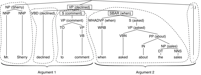
We use three types of features: Word pairs, produc-tion rules from the parse tree, as well as features en-coding the lexico-syntactic context at the border be-tween two units of text (Soricut and Marcu, 2003). Our word pairs are lemmatized using the Wordnet-based lemmatizer of NLTK (Loper and Bird, 2002). Figure 1 shows the parse tree for a sentence com-posed of two discourse units, which serve as argu-ments of a discourse relation we want to generate a feature vector from. Lexical heads have been calcu-lated using the projection rules of Magerman (1995), and annotated between brackets. Surrounded by dots is, for each argument, the minimal set of sub-parse trees containing strictly all the words of the argument.

We first extract all possible lemmatized word-pairs from the two arguments, such as(Mr., when), (decline, ask)or(comment, sale). Next, we extract from left and right argument separately, all produc-tion rules from the sub-parse trees, such as NP 7→ NNP NNP, NNP7→“Sherry” or TO7→“to”.

Finally, we encode in our features three nodes of the parse tree, which capture the local context at the connection point between the two arguments: The first node, which we callNw, is the highest

ances-tor of the first argument’s last wordw, and is such thatNw’s right-sibling is the ancestor of the second

argument’s first word. Nw’s right-sibling node is

calledNr. Finally, we callNpthe parent ofNw and

Nr. For each node, we encode in the feature

vec-tor its part-of-speech (POS) and lexical head. For instance, in Figure 1, we have Nw = S(comment),

Nr = SBAR(when), andNp = VP(declined). In the

PDTB, certain discourse relations have disjoint ar-guments. In this case, as well as in the case where the two arguments belong to different sentences, the nodesNw,Nr,Npcannot be defined, and their

cor-responding features are given the value zero.

4 Experiments

The proposed method is independent of any partic-ular classification algorithm. Because our goal is strictly to evaluate the relative benefit of employing

the proposed method, and not the absolute perfor-mance when used with a specific classification algo-rithm, we select a logistic regression classifier, for its simplicity. We use the multi-class logistic regression (maximum entropy model) implemented in the Clas-sias toolkit (Okazaki, 2009). Regularization param-eters are set to their default value of one and are fixed throughout the experiments described in the paper.

To create our unlabeled dataset, we use sentences extracted from the English Wikipedia2_{, as they are} freely available and relatively easy to collect. For further extraction of syntactic features, these sen-tences are automatically parsed using the Stanford parser (Klein and Manning, 2003). Then, they are segmented into elementary discourse units (EDUs) using our sequential discourse segmenter (Hernault et al., 2010). The relatively high performance of this RST segmenter, which has an F-score of 0.95

compared to that of 0.98 between human annota-tors (Soricut and Marcu, 2003), is acceptable for this task. We collect and parse100000 sentences from random Wikipedia articles. As there is no segmen-tation tool for the PDTB framework, we assume that co-occurrence information taken fromEDUs created using a RST segmenter is also useful for extending feature vectors of PDTB relations. Unless other-wise noted, the experiments presented in the rest of this paper are done using those100000unlabeled in-stances.

In the unlabeled data, any two consecutive course units might not always be connected by a dis-course relation. Therefore, we introduce an artificial NONErelation in the training set, in order to facil-itate this. Instances of the NONE relation are gen-erated randomly by pairing consecutive discourse units which are not connected by a discourse relation in the training data. NONEis also learnt as a separate discourse relation class by the multi-class classifica-tion algorithm. This enables us to detect discourse units between which there exist no discourse rela-tion, thereby improving the classification accuracy for other relation types.

We follow the common practice in discourse re-search for partitioning the discourse corpora into training and test set. For the RST classifier, the dedicated training and test sets of the RSTDT are

NP (Sherry)

S (declined)

VP (declined)

NNP NNP

declined VBD (declined)

Mr. Sherry to

VP (comment)

comment when asked about the sales

TO VP

SBAR (when)

WHADVP (when)

WRB

S (asked)

VP (asked)

VBN PP (about)

IN NP (sales)

DT NNS

. . (.)

Argument 1 Argument 2

VB S (comment)

Figure 1: Two arguments of a discourse relation, and the minimum set of subtrees that contain them—lexical heads are indicated between brackets.

employed. For the PDTB classifier, we conform to the guidelines of Prasad et al. (2008b, 5): The por-tion of the corpus corresponding to secpor-tions 2–21 of the WSJ is used for training the classifier, while the portion corresponding to WSJ section 23 is used for testing. In order to extract syntactic features, all training and test data are furthermore aligned with their corresponding parse trees in the Penn Treebank (Marcus et al., 1993).

Because in the PDTB an instance can be annotated with several discourse relations simultaneously—called ‘senses’ in Prasad et al. (2008b)—for each instance with n senses in the corpus, we create n identical feature vectors, each being labeled by one of the instance’s senses. However, in the RST framework, only one relation is allowed to hold between two EDUs. Conse-quently, each instance from the RSTDT is labeled with a single discourse relation, from which a single feature vector is created. For RSTDT, we extract25078training vectors and1633test vectors. For PDTB we extract 49748 training vectors and

1688 test vectors. There are 41 classes (relation types) in the RSTDT relation classification task, and 29 classes in the PDTB task. For the PDTB, we selected level-two relations, because they have better expressivity and are not too fine-grained. We experimentally set the entropy-based feature selection parameter to N = 5000. With large N values, we must store and process large feature co-occurrence matrices. For example, doubling the number of selected features, N to 10000 did

not improve the classification accuracy, although it required 4GB of memory to store the feature co-occurrence matrix.

Figure 2 shows the number of features that occur in test data but not in labeled training data, against the number of training instances. It can be seen from Figure 2 that, with less training data available to the classifier, we can potentially obtain more informa-tion regarding features by looking at unlabeled data. However, when the training dataset’s size increases, the number of features that only appear in test data decreases rapidly. This inverse relation between the training dataset size and the number of features that only appear in test data can be observed in both RSTDT and PDTB datasets. For a training set of

100 instances, there are 23580 unseen features in the case of RSTDT, and27757in the case of PDTB. The number of unseen features is halved for a train-ing set of1800instances in the case of RSTDT, and for a training set of 1300 instances in the case of PDTB. Finally, when selecting all available training data, we count only1365unseen test features in the case of RSTDT, and87in the case of PDTB.

re-0 5000 10000 15000 20000 25000

Number of training instances

0 5000 10000 15000 20000 25000 30000

Number of unseen test features

RSTDT PDTB

Figure 2: Number of features seen only in the test set, as a function of the number of training instances used.

lation types we use macro-averaged F-score as the preferred evaluation metric for this task.

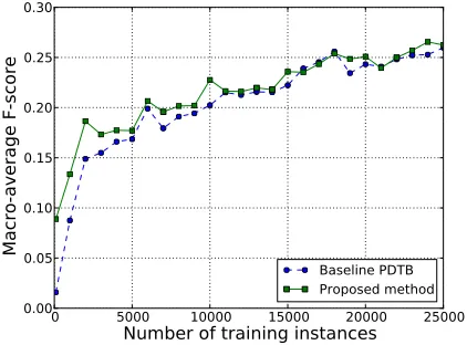
We train a multi-class logistic regression model without extending the feature vectors as a baseline method. This baseline is expected to show the ef-fect of using the proposed feature vector extension approach for the task of discourse relation learn-ing. Experimental results on RSTDT and PDTB datasets are depicted in Figures 3 and 4. From these figures, we see that the proposed feature ex-tension method outperforms the baseline for both RSTDT and PDTB datasets for the full range of training dataset sizes. However, whereas the differ-ence of scores between the two methods is obvious for small amounts of training data, this difference progressively decreases as we increase the amount of training data. Specifically, with100training in-stances, the difference between baseline and pro-posed method is the largest: For RSTDT, the base-line has a macro-averaged F-score of0.084, whereas the the proposed method has a macro-averaged F-score of 0.189(ca.119% increase in F-score). For PDTB, the baseline has an F-score of 0.016, while the proposed method has an F-score of0.089(459%

increase). The difference of scores between the two methods then progressively diminishes as the num-ber of training instances is increased, and fades be-yond10000training instances. The reason for this behavior is given by Figure 2: For a small number of training instances, the number of unseen features in training data is large. In this case, the feature

vec-tor extension process is comprehensive, and score can be increased by the use of unlabeled data. When more training data is progressively used, the num-ber of unseen test features sharply diminishes, which means feature vector extension becomes more lim-ited, and the performance of the proposed method gets progressively closer to the baseline. Note that we plotted PDTB performance up to 25000 train-ing instances, as the number of unseen test features becomes so small past this point that the perfor-mances of the proposed method and baseline are identical. Using all PDTB training data (49748 in-stances), both baseline and proposed method reach a macro-average F-score of0.308.

0 5000 10000 15000 20000 25000

Number of training instances

0.05 0.10 0.15 0.20 0.25 0.30

Macro-average F-score

Baseline RSTDT Proposed method

Figure 3: Macro-average F-score (RSTDT) as a function of the number of training instances used.

0 5000 10000 15000 20000 25000

Number of training instances

0.00 0.05 0.10 0.15 0.20 0.25 0.30

Macro-average F-score

Baseline PDTB Proposed method

#Tr=1 #Tr=2 #Tr=3 #Tr=5 #Tr=7

Relation name B. P.M. B. P.M. B. P.M. B. P.M. B. P.M.

Attribution[N][S] – 0.127 – 0.237 – 0.458 0.038 0.290 0.724 0.773

Attribution[S][N] – 0.597 – 0.449 0.009 0.639 0.250 0.721 0.579 0.623

Background[N][S] – 0.113 – – – 0.036 – 0.095 – 0.089

Cause[N][S] – – – 0.128 – – – 0.034 0.057 0.187

Comparison[N][S] – 0.118 – 0.037 – – 0.133 0.130 0.143 0.031

Condition[N][S] – 0.041 – 0.136 – 0.113 – 0.154 0.242 0.152

Condition[S][N] – – – 0.122 0.133 0.148 0.214 0.233 0.390 0.308

Contrast[N][N] – – – 0.086 – 0.073 0.050 0.111 – 0.109

Contrast[N][S] – 0.071 – – – 0.188 – 0.087 – 0.136

Elaboration[N][S] – 0.134 – 0.126 0.004 0.067 0.004 0.340 – 0.165

Enablement[N][S] – – – 0.462 – 0.579 0.115 0.423 0.419 0.438

Joint[N][N] – 0.030 – 0.015 – – 0.016 0.059 0.015 0.155

Manner-Means[N][S] – – – 0.056 – 0.103 0.345 0.372 0.412 0.383

Summary[N][S] – 0.429 – 0.453 0.080 0.358 – 0.349 0.154 0.471

Temporal[N][S] – 0.158 – – – 0.091 – 0.052 0.204 0.101

Accuracy 0.000 0.110 0.000 0.105 0.004 0.146 0.034 0.222 0.122 0.213

Macro-average F-score 0.000 0.060 0.000 0.069 0.008 0.101 0.038 0.118 0.107 0.134

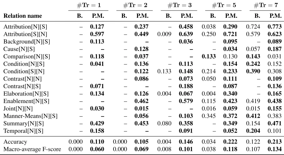
Table 1: F-scores for RSTDT relations, using a training set containing #Tr instances of each relation. B. indicates F-score for baseline, P.M. for the proposed method. A boldface indicates the best classifier for each relation.

Although the distribution of discourse relations in RSTDT and PDTB is not uniform, it is possi-ble to study the performance of the proposed method when all relations are made equally rare. We evalu-ate performance on artificially-creevalu-ated training sets containing an equal amount of each discourse rela-tion. Table 1 contains the F-score for each RSTDT relation, using training sets containing respectively one, two, three, five and seven instances of each relation. For space considerations, only relations with significant results are shown. We observe that, when using respectively one and two instances of each relation, the baseline classifier is unable to de-tect any relation, and has a macro-average F-score of zero. Contrastingly, the classifier built with fea-ture vector extension reaches in those cases an F-score of 0.06. Furthermore, when employing the proposed method, certain relations have relatively high F-scores even with very little labeled data: With one training instance, ATTRIBUTION[S][N] has an

F-score of0.597, while SUMMARY[N][S] has an F-score of0.429. With three training instances, EN

-ABLEMENT[N][S] has an F-score of0.579. When

the amount of each relation is increased, the baseline classifier starts detecting more relations. In all cases, the proposed method performs better in terms of ac-curacy and macro-average F-score. With a train-ing set containtrain-ing seven instances of each relation, the baseline’s macro-average F-score is starting to get closer to the extended classifier’s, with superior performances for several relations, such as COM

-PARISON[N][S], CONDITION[N][S], and TEMPO

-RAL[N][S]. Still, in this case, the extended

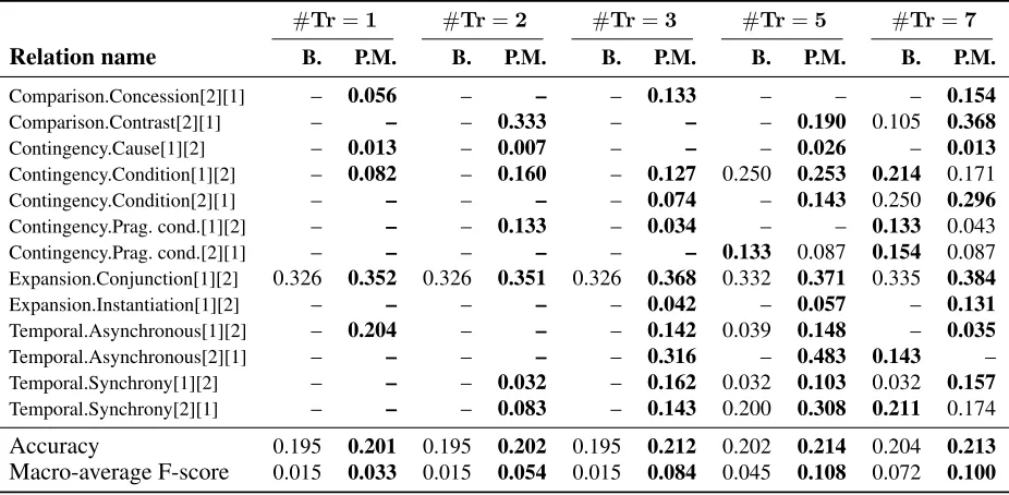
classi-fier’s accuracy is higher than the baseline (0.213 ver-sus0.122). Table 2 summarizes the outcome of the same experiments performed on the PDTB dataset. The results exhibit a similar trend, despite the base-line classifier having a relatively high accuracy for each case.

#Tr=1 #Tr=2 #Tr=3 #Tr=5 #Tr=7

Relation name B. P.M. B. P.M. B. P.M. B. P.M. B. P.M.

Comparison.Concession[2][1] – 0.056 – – – 0.133 – – – 0.154

Comparison.Contrast[2][1] – – – 0.333 – – – 0.190 0.105 0.368

Contingency.Cause[1][2] – 0.013 – 0.007 – – – 0.026 – 0.013

Contingency.Condition[1][2] – 0.082 – 0.160 – 0.127 0.250 0.253 0.214 0.171

Contingency.Condition[2][1] – – – – – 0.074 – 0.143 0.250 0.296

Contingency.Prag. cond.[1][2] – – – 0.133 – 0.034 – – 0.133 0.043

Contingency.Prag. cond.[2][1] – – – – – – 0.133 0.087 0.154 0.087

Expansion.Conjunction[1][2] 0.326 0.352 0.326 0.351 0.326 0.368 0.332 0.371 0.335 0.384

Expansion.Instantiation[1][2] – – – – – 0.042 – 0.057 – 0.131

Temporal.Asynchronous[1][2] – 0.204 – – – 0.142 0.039 0.148 – 0.035

Temporal.Asynchronous[2][1] – – – – – 0.316 – 0.483 0.143 –

Temporal.Synchrony[1][2] – – – 0.032 – 0.162 0.032 0.103 0.032 0.157

Temporal.Synchrony[2][1] – – – 0.083 – 0.143 0.200 0.308 0.211 0.174

Accuracy 0.195 0.201 0.195 0.202 0.195 0.212 0.202 0.214 0.204 0.213

Macro-average F-score 0.015 0.033 0.015 0.054 0.015 0.084 0.045 0.108 0.072 0.100

Table 2: F-scores for PDTB relations.

not bring any change in F-score or accuracy. In-deed, as the number of unknown features is low, feature vector extension is very limited, and does not improve the performance compared to the base-line. Then, a progressive increase of both accuracy and macro-average F-score is observed, as the num-ber of unseen test features is incremented. For in-stance, for 8500 unseen test features, the macro-average F-score increase (resp. accuracy increase) is25%(resp.2.5%), while it is20%(resp.1%) for

11000 unseen test instances. These values reach a maximum of119%macro-average F-score increase, and 66% accuracy increase, when 23500 features unseen during training are present in test data. This situation corresponds in Figures 3 and 4 to the case of very small training sets. The bottom subfigure of Figure 2, for the case of PDTB, reveals a sim-ilar tendency. The macro-average F-score increase (resp. accuracy increase) is negligible for1000 un-seen test features, while this increase is21%for both macro-average F-score and accuracy in the case of

9700unseen test features, and459%(resp. 630% for accuracy) when28000unseen features are found in test data. This shows that the proposed method is useful when large numbers of features are missing from the training set, which corresponds in practice to small training sets, with few training instances for each relation type. For large training sets, most

fea-tures are encountered by the classifier during train-ing, and feature vector extension does not bring use-ful information.

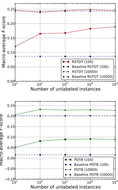
We empirically evaluate the effect of using differ-ent amounts of unlabeled data on the performance of the proposed method. We use respectively100and

10000labeled training instances, create feature co-occurrence matrices with different amounts of unla-beled data, and evaluate the performance in relation classification. Experimental results for RSTDT are illustrated in Figure 6 (top). From Figure 6 it appears clearly that macro-average F-scores improve with increased number of unlabeled instances. However, the benefit of using larger amounts of unlabeled data is more pronounced when only a small number of la-beled training instances are employed (ca.100). In fact, with100labeled training instances, the maxi-mum improvement in F-score is119%(corresponds to using all our100000unlabeled instances). How-ever, the maximum improvement in F-score with

10000labeled training instances is small, only2.5%

(corresponds to10000unlabeled instances).

us-0 5000 10000 15000 20000 25000

Number of unseen features in test data

0 20 40 60 80 100 120

Score change over baseline (%)

Accuracy change RSTDT Macro-av. F-score change RSTDT

0 5000 10000 15000 20000 25000 30000

Number of unseen features in test data

0 100 200 300 400 500 600 700

Score change over baseline (%)

Accuracy change PDTB Macro-av. F-score change PDTB

Figure 5: Score change as a function of unseen test fea-tures for RSTDT (top) and PDTB (bottom).

ing unlabeled data is more obvious when the num-ber of labeled training instances is small. In par-ticular, with 100 training instances, the maximum improvement in F-score is 459% (corresponds to

100000unlabeled instances). However, with10000

labeled training instances the maximum improve-ment in F-score is 15% (corresponds to 100 unla-beled instances). These results confirm that, on the one hand performance improvement is more promi-nent for smaller training sets, and that on the other hand, performance is increased when using larger amounts of unlabeled data.

5 Conclusion

We presented a semi-supervised method which ex-ploits the co-occurrence of features in unlabeled data, to extend feature vectors during training and testing in a discourse relation classifier. Despite the

0.00 0.05 0.10 0.15 0.20 0.25

Macro-average F-score

101 ₁₀2 ₁₀3 ₁₀4 ₁₀5

Number of unlabeled instances

RSTDT (100) Baseline RSTDT (100) RSTDT (10000) Baseline RSTDT (10000)

0.10 0.05 0.00 0.05 0.10 0.15 0.20 0.25

Macro-average F-score

101 ₁₀2 ₁₀3 ₁₀4 ₁₀5

Number of unlabeled instances

PDTB (100) Baseline PDTB (100) PDTB (10000) Baseline PDTB (10000)

Figure 6: Macro-average F-score for RSTDT (top) and PDTB (bottom), for 100 and 10000 training instances, against the number of unlabeled instances.

References

R. Basili, M. Cammisa, and A. Moschitti. 2006. A se-mantic kernel to classify texts with very few training examples. Informatica (Slovenia), 30(2):163–172. S. Bloehdorn, R. Basili, M. Cammisa, and A. Moschitti.

2006. Semantic kernels for text classification based on topological measures of feature similarity. InProc. of ICDM’06, pages 808–812.

L. Carlson, D. Marcu, and M. E. Okurowski. 2001. Building a discourse-tagged corpus in the framework of Rhetorical Structure Theory. Proc. of Second SIG-dial Workshop on Discourse and Dialogue-Volume 16, pages 1–10.

N. Cristianini, J. Shawe-Taylor, and H. Lodhi. 2002. La-tent semantic kernels. Journal of Intelligent Informa-tion Systems, 18:127–152.

S. C. Deerwester, S. T. Dumais, T. K. Landauer, G. W. Furnas, and R. A. Harshman. 1990. Indexing by latent semantic analysis. Journal of the American Society of Information Science, 41(6):391–407.

D. A. duVerle and H. Prendinger. 2009. A novel dis-course parser based on Support Vector Machine clas-sification. InProc. of ACL’09, pages 665–673. H. Fang. 2008. A re-examination of query expansion

us-ing lexical resources. InProc. of ACL’08, pages 139– 147.

C. Fellbaum, editor. 1998. WordNet: An electronic lexi-cal database. MIT Press.

H. Hernault, D. Bollegala, and M. Ishizuka. 2010. A sequential model for discourse segmentation. InProc. of CICLing’10, pages 315–326.

D. Klein and C. D. Manning. 2003. Fast exact inference with a factored model for natural language parsing. In Advances in Neural Information Processing Systems, volume 15. MIT Press.

Z. Lin, M-Y. Kan, and H. T. Ng. 2009. Recognizing im-plicit discourse relations in the Penn Discourse Tree-bank. InProc. of EMNLP’09, pages 343–351. E. Loper and S. Bird. 2002. NLTK: The natural

lan-guage toolkit. InProc. of ACL’02 Workshop on Effec-tive tools and methodologies for teaching natural lan-guage processing and computational linguistics, pages 63–70.

D. M. Magerman. 1995. Statistical decision-tree models for parsing. Proc. of ACL’95, pages 276–283.

W. C. Mann and S. A. Thompson. 1988. Rhetorical Structure Theory: Toward a functional theory of text organization. Text, 8(3):243–281.

C. D. Manning and H. Sch¨utze. 1999. Foundations of Statistical Natural Language processing. MIT Press. D. Marcu and A. Echihabi. 2002. An unsupervised

ap-proach to recognizing discourse relations. InProc. of ACL’02, pages 368–375.

D. Marcu. 2000. The Theory and Practice of Discourse Parsing and Summarization. MIT Press.

M. P. Marcus, M. A. Marcinkiewicz, and B. Santorini. 1993. Building a large annotated corpus of En-glish: The Penn Treebank. Computational Linguistics, 19(2):313–330.

N. Okazaki. 2009. Classias: A collection of machine-learning algorithms for classification. http://

www.chokkan.org/software/classias/.

B. Pang and L. Lee. 2008. Opinion mining and senti-ment analysis. Foundations and Trends in Information Retrieval, 2(1-2):1–135.

E. Pitler, M. Raghupathy, H. Mehta, A. Nenkova, A. Lee, and A. Joshi. 2008. Easily identifiable discourse rela-tions. InProc. of COLING’08 (Posters), pages 87–90. E. Pitler, A. Louis, and A. Nenkova. 2009. Automatic sense prediction for implicit discourse relations in text. InProc. of ACL’09, pages 683–691.

P. Piwek, H. Hernault, H. Prendinger, and M. Ishizuka. 2007. Generating dialogues between virtual agents au-tomatically from text. InProc. of IVA’07, pages 161– 174.

R. L. Plackett. 1983. Karl Pearson and the chi-squared test. International Statistical Review / Revue Interna-tionale de Statistique, 51(1):59–72.

R. Prasad, N. Dinesh, A. Lee, E. Miltsakaki, L. Robaldo, A. Joshi, and B. Webber. 2008a. The Penn Discourse TreeBank 2.0. InProc. of LREC’08.

R. Prasad, E. Miltsakaki, N. Dinesh, A. Lee, A. Joshi, L. Robaldo, and B. Webber. 2008b. The Penn Dis-course Treebank 2.0 annotation manual. Technical re-port, University of Pennsylvania Institute for Research in Cognitive Science.

G. Salton and C. Buckley. 1983. Introduction to Modern Information Retrieval. McGraw-Hill Book Company. G. Siolas and F. d’Alch´e-Buc. 2000. Support Vector

Ma-chines based on a semantic kernel for text categoriza-tion. InProc. of IJCNN’00, volume 5, page 5205. S. Somasundaran, G. Namata, J. Wiebe, and L. Getoor.

2009. Supervised and unsupervised methods in em-ploying discourse relations for improving opinion po-larity classification. In Proc. of EMNLP’09, pages 170–179.

R. Soricut and D. Marcu. 2003. Sentence level discourse parsing using syntactic and lexical information. Proc. of NA-ACL’03, 1:149–156.