Abstract—A novel approach to plan an optimum motion of
redundant robot manipulators for a predefined end-effector trajectory using genetic algorithms (GA) is presented. The efficiency of the proposed approach, without loss of generality, is demonstrated through a simulation carried out on a planar 6-DOF robot manipulator. The approach benefits from two key features. First, the method of data representation which guarantees the satisfaction of joints angle limits, and second the conversion of considered model’s 6-DOF construction to 4-DOF construction along with an additional binary value which guarantees the exact placement of the end-effector on the predefined trajectory. Comparison with three other approaches shows that the result of the presented solution is substantially better. In addition the difference of two kinds of Random Number Generator (RNG) is addressed. It is shown that using RNG with normal distribution leads to faster convergence of the proposed algorithm than RNG with uniform distribution.
Index Terms—Genetic Algorithms, Manipulator, Motion
Planning, Trajectory Tracking
I. INTRODUCTION
Recently, there has been an increased research interest in the development of efficient procedures to solve the inverse kinematics problem of redundant robot manipulators. In general, solving the inverse kinematics problem of redundant robots is not trivial since the necessary mapping from the task coordinates to the joint coordinates is not one to one, and yields an infinite of solutions [1, 2]. Redundant robot manipulators can provide a better ability to avoid singular configuration and the excessive velocities and accelerations encountered at singularities [3].
Generally, there are three main approaches for trajectory planning for redundant manipulators, pseudo-inverse of Jacobian matrix, variational approach, and optimization techniques based on the direct kinematics [4].
Davidor [5] applied a GA to generate the robot trajectory by finding the inverse kinematics for predefined end-effector robot paths. A trajectory of a 3-link planar redundant robot is simulated by minimizing the sum of the position errors at each of the knot points along the path. Yun and Xi [6] presented a new method for optimum motion planning based on an improved genetic algorithm. This approach incorporates kinematics constraints, dynamics constraints as
Manuscript received March 31, 2008.
Amir Homayoun Javadi A. is with Robotics and Automation Lab, Noise Company and National Olympic and Paralympics Academy of Iran, Tehran, Iran (phone: +98 912 182 0929; e-mail: [email protected]).
well as control constraints. Simulation results for two and three DOF robots were presented. Hirakawa and Kawamura [7] proposed a combination of B-spline trajectory generation and steepest gradient optimization to design an optimal motion planning for redundant manipulators. However, the proposed optimization approach needs to determine the gradients of the objective function. McAvoy et al. [2] proposed an approach utilizing genetic algorithms for optimal point-to-point motion planning for kinematically redundant manipulators to satisfy both the initial conditions and some other specified criteria. Their approach combines B-spline curves for the generation of smooth trajectories with genetic algorithms for optimal solution. Ata and Myo [4] has proposed an optimal point-to-point trajectory planning for planar redundant manipulator. Their main objective was to minimize the sum of the position error of the end-effector at each intermediate point along the trajectory so that the end-effector can track the prescribed trajectory accurately. They introduced an algorithm combining Genetic Algorithm and Pattern Search as a Generalized Pattern Search GPS to design the optimal trajectory. To verify the proposed algorithm, simulations for a 3-DOF planar manipulator with different end-effector trajectories have been carried out.
Our proposed GA optimization mechanism differs from the mentioned methods in a number of ways. The first difference lies on robot’s model alternation in order to computationally track the end-effector trajectory without any evolution, so the end-effector would be exactly placed on the predefined trajectory. Therefore, there would be no tracking error. The second difference is that the joints angle are not manipulated directly, rather they are accessed through a mapping function, (8), which maps real values ]−∞..+∞[ to lower and upper boundaries of joints angle. Thus the joints angle limits are satisfied without any conditioning statement. Moreover it is shown that in this special type of problem, selecting a special kind of Random Number Generator (RNG) can improve the optimization process.
The remainder of the paper is organized as following: Section 0 II gives the robot’s model and the method of model manipulation. Section III gives a brief overview of the concept of GA in each building block of the algorithm and presents the proposed GA solution. Section IV demonstrates and discusses the efficiency of the proposed GA through an experiment. In the same section, the performance of the proposed solution is compared to that of three previous approaches. Finally, Section V summarizes the contribution of the paper.
Manipulator Redundancy Reduction as a Tool
for Reinforcing Motion Planning Using
Genetic Algorithms
II. THE MANIPULATOR’S MODEL
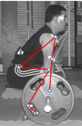
[image:2.612.117.251.46.251.2]A 6-DOF robot manipulator is considered throughout the simulation. The model and the end-effector trajectory is adopted from human body during weightlifting task, Fig. 1, in which the end-effector trajectory is the trajectory of barbell in a sample snatch lift. Table I shows the links length along with the links mass. It is supposed that center of mass of each link is placed on the geometric center of itself.
Table I. Links name along with Links length and mass Link Length (cm) Mass (kg) 1
l , foot 13.20 3.04
2
l , shank 38.57 9.76
3
l , thigh 31.10 21
4
l , trunk 50.10 59.85
5
l , upper-arm 26.89 5.88 6
l , lower-arm 42.01 4.62
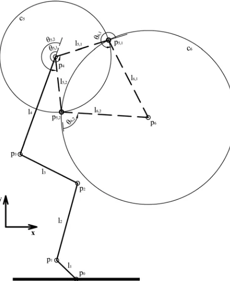
[image:2.612.349.515.48.244.2]The proposed model is shown in Fig. 2. θj, j=1..6, are joints angle based on Denavit-Hartenberg (DH) representation. Table II shows the joints angle limits based on DH representation for the sample proposed manipulator. Values exceeding 360° indicate the portion of the unit circle between θj,min and θj,max, positive horizontal axis, as shown in Fig. 3.
Table II. Joints angle limits based on Denavit-Hartenberg representation 1
θ toe
2 θ ankle
3 θ knee
4 θ hip
5 θ shoulder
6 θ elbow Min 90° 287° 5° 224° 191° 280° Max 150° 348° 134° 378° 377° 390°
As mentioned, one of the key features of our approach lies on the method of model conversion, in which, to ensure the trajectory tracking task, two degrees of freedom of the model are replaced with a single binary alternation and as a consequence the problem is reduced to define four real value
joints angle along with a single binary value. The definition of model’s control parameters is converted from 6 rotary parameters to 4 rotary parameters and one binary value to fulfill the trajectory tracking task. The other two undefined joints angle are calculated geometrically in the sense to place the end-effector on the desired position. Fig. 4 shows the robot with two different configurations as below
⎩ ⎨ ⎧ =
} , , , , , {
} , , , , , , { ion Configurat
1 , 6 1 , 5 4 3 2 1
6 1 , 5 4 3 2 1 0
1 θ θ θ θ θ θ
p p p p p p p
(1a)
⎩ ⎨ ⎧ =
} , , , , , {
} , , , , , , { ion Configurat
2 , 6 2 , 5 4 3 2 1
6 2 , 5 4 3 2 1 0
2 θ θ θ θ θ θ
p p p p p p p
(1b) in which the points pi, i=1..6, are defined as below,
T
p0=[0,0] (2)
T i
j j i
j j i
i i p l
p ⎥
⎦ ⎤ ⎢
⎣ ⎡ +
=
∑
∑
= =
− cos( ),sin( )
1 1
1 θ θ , i=1..4 (3)
κ τ = Τ = 6
p (4)
in which θj are joints angle based on DH representation as shown in Fig. 2. p0 is the robot’s base point, positioned at the position T
] 0 , 0
[ . Ττ =κ shows the desired position of end-effector on the trajectory in the instance of time κ . Predefined trajectory is broken into discrete intervals of time denoted by κ, κ=0..n, which n shows the total number of Fig. 1. Weightlifter at the initial state. Links are shown in red lines and joints
are shown in blue circles.
Fig. 2. Manipulator’s model; Joints angle are based on DH representation.
[image:2.612.355.503.277.395.2][image:2.612.95.275.417.517.2] [image:2.612.69.299.629.682.2]
discrete time steps. θj, j=1..4, are know in each frame of time, using the GA solution, p0 is a fixed point and p6 is placed on a predefined position on the trajectory in each instance of time, τ . p5, θ5 and θ6 can be calculated using the system of equations below,
⎪⎩ ⎪ ⎨ ⎧
= − + −
= − + −
2 6 2 6 5 2 6 5
2 5 2 4 5 2 4 5
) ( ) (
) ( ) (
l y y x x
l y y x x
(5) which xi and yi shows the horizontal and vertical position
of joint position pi, respectively. System of equations 5 has two pare of solutions if p4,p6 <l5+l6 , two configurations 0 and 1, has one pair of solution if p4,p6 =l5+l6 and has no real value solution if p4,p6 >l5+l6, where pn,pm stands for the Euclidean distance between points pn and pm. Joints angle θ5 and θ6 must be calculated according to joints position p4, p5 and p6 to validate the joints angle limits due to Table I. The condition to be met is as following,
⎩ ⎨ ⎧
° > <
∨ <
° ≤ ≤
∧ ≤
360
for )) 360
mod
( (
) (
360
for )
(
) (
max , max
, , , min ,
max , max
, , , min ,
j j
c j c j j
j j
c j c j j
θ θ
θ θ θ
θ θ
θ θ θ
(6) in which j=5..6 and c=1..2 and θj,c is the calculated
angle. (a mod b) means the remainder, on division of a by
b. For the sample configurations shown in Fig. 4, θ6,2 is obviously out of the range θ6,min =280° and θ6,max =390°, so the configuration shown in (1b) is not valid. θ5,1=307°
and θ6,1=280° are both in the valid range defined in Table
II, so for the predefined trajectory and the at hand values
} , , ,
{θ1θ2θ3θ4 or respectively {p0,p1,p2,p3,p4}, the only feasible configuration is (1a).
In the case of p4,p6 <l5+l6, two possible positions of 5
p are named as p5,1 and p5,2 and joints angle θ5 and θ6 are denoted as θ5,1, θ6,1 and θ5,2, θ6,2. For p4,p6 =l5+l6, indeed, we have two positions p5,1 and p5,2 which
2 , 5 1 ,
5 p
p = .
III. THE GENETIC ALGORITHMS SOLUTION
Given the manipulator’s model and the predefined end-effector trajectory, the GA plans an optimum sequence of configurations in the sense of minimizing the total consumed energy. In the following the proposed GA solution is presented.
A. The Representation Mechanism
The first, and perhaps the most critical aspect in designing a GA for a specific optimization problem is the basic mechanism that links the GA to the solution space of the problem [1]. This mechanism consists of choosing a method to represent a solution to the real problem as a finite-length string over a specific alphabet, the chromosome. The second key feature of our approach is the method of data representation, the content of each chromosome.
In our approach, each member of the GA consists of one initial configuration, τ=0 , along with a sequence of configurations in which the sequence of movements of the manipulator is stored. The mentioned sequence contains the configurations from the frame next to the beginning to the end of the trajectory, τ =1..n.
The chromosome encoding the initial configuration consists of a single binary value, ν0τ=0 indicating the configuration and four elements νrτ=0, r=1..4, which each element indicates the quantity of σj,0 in the function
) ( j,0
j
S σ , j=1..4, (8). The function Sj(σj,κ) incorporates a
sigmoid function, 1/(1+exp(−σj,κ)), in order to map the
random values, σj,κ , to degree values, θjτ=κ . The configuration here denotes the selection of the position of joint number 5, p5,1 or p5,2.
The sequence of chromosomes encoding the sequence of configurations throughout the rest of the trajectory contains a single binary value indicating the configuration type, ν0τ=κ, and four elements νrτ=κ , r=1..4 , which each element contributes in the calculation of the value σj,κ which is used in the function Sj(σj,κ), j=1..4, as shown below,
( )
∑ =
= = κ
ε τ κ
κ ν
σ 0
, j
j , (7)
) exp( 1
1 ). (
) (
, min
, max , min , ,
κ
κ θ θ θ σ
σ
j j
j j j j
S
− + −
+
= (8)
) ( ,κ κ
τ σ
[image:3.612.72.299.58.335.2]θj = =Sj j . (9)
Fig. 4. Two possible configurations (1a) and (1b) using predefined positions
} , , , , ,
Using the above formulation has two key benefits. The first benefit lies on the manner the joints angle limits are served. Using the sigmoid function, (8), guarantees the placement of the joint angle value in the boundary
] ..
[θj,min θj,max . At extremes, σj,κ →+∞ and σj,κ →−∞, the value of Sj(σj,κ) would be θj,max and θj,min, respectively. In this way, the need for evaluating several if statements, validating the joints angle limits is eliminated.
The following summarizes the notations defined above. A member is defined as,
⎥ ⎥ ⎥ ⎥ ⎥ ⎦ ⎤ ⎢ ⎢ ⎢ ⎢ ⎢ ⎣ ⎡ = = = = n τ τ τ μ v v v M M 1 0 (10)
in which Mμ, μ=1..m, stands for the member μ within a generation, and
m
is the total number of members in each generation. vτ =κ is a chromosome concerning a single instance of time τ =κ, defining the configuration of the robot as shown below,]
[ 0τκ 1τ κ 2τ κ 3τκ 4τκ
κ
τ= =ν = ν = ν = ν = ν =
v (11)
where ν0τ=κ is a binary value, either 0 or 1, selecting one of the configurations (1a) or (1b), and νrτ=κ , r=1..4, defines a randomly generated value used in the calculation of
κ
σj, , (7). Finally the values σj,κ are applied to the function
) (σj,κ
j
S to calculate the joints angle in each instance of time
n
.. 0
=
τ , (8).
B. Random Number Generation
Chromosomes, as noted in (11), consist of 5 random numbers defining the random binary configuration, for ν0, and random joint angle variations inputted to equations (7)-(9), for νr, r=1..4. The Random Number Generator (RNG), ℜ, must satisfy the condition below,
1 ) ( = ℜ
∫
+∞ ∞− pdp (12)
which ℜ(p) is the probability density function (pdf) of ℜ at point p.
A threshold value for the assignment of binary configuration value ν0 must be assigned due to ℜ(p) in order to satisfy the equation below,
2 / 1 ) ( )
( = ℜ =
ℜ
∫
∫
+∞ ∞ − T T dp p dpp (13)
to give an equal chance to both sides of binary value. T is the threshold value.
Two different kinds of ℜ are proposed. ℜ are supposed to be with uniform pdf and with normal pdf,
ℜ
u and ℜn respectively. The two proposed RNGs, are shown below,⎪ ⎪ ⎩ ⎪ ⎪ ⎨ ⎧ = − ℜ ⋅ = ⎩ ⎨ ⎧ > ℜ ≤ ℜ = ℜ 4 .. 1 for 2 0 for 5 . 0 if 1 5 . 0 if 0 , r r u u u u u r u ρ ρ (14) ⎪ ⎪ ⎩ ⎪ ⎪ ⎨ ⎧ = ℜ ⋅ = ⎩ ⎨ ⎧ > ℜ ≤ ℜ = ℜ 4 .. 1 for 0 for 0 if 1 0 if 0 , r r n n n n r n ρ (15)
where ρn and ρu are constant scaling values. Threshold values for ℜu,0 and ℜn,0 are Tu =0.5 and Tn =0 , respectively. ℜu(p) and ℜn(p) are defined as below,
⎩ ⎨ ⎧ ≥ ≤ < < − = ℜ b p a p b p a a b p u or for 0 for ) /( 1 )
( (16)
⎟⎟ ⎠ ⎞ ⎜⎜ ⎝ ⎛− − =
ℜ 2 2
2 ) ( exp 2 1 ) ( σ μ π σ x p
n (17)
where a and b, a<b, are the minimum and maximum values of ℜu(p), respectively and
2
σ and μ are variance and mean values of ℜn(p), respectively. Two mentioned
RNGs are compared within a simulation. It is shown that the type and the values of the parameters of function ℜ have a critical role in the performance of the GA. Several configurations are proposed and compared in chapter III section F.
C. The Initial Population
The initial population and new members in each generation are generated randomly. Generating members with some criteria applied to the initial configuration can drastically reduce the computation time required by the GA. It is shown that minimizing the static torque applied to each joint at the initial configuration, τ =0, improves the overall performance of the GA.
The initial population and new members in each generation are generated randomly. Mμ is generated using a proposed ℜ and the feasibility of Mμ is checked against two criteria, first p4,p6 ≤l5+l6 and second, joint angle limits for θ5 and θ6. Both the criteria must be satisfied in order to keep the generated member, Mμ, in the generation.
D. The Evaluation Mechanism
In an optimization problem, the fitness function corresponds to the objective function which must be optimized. Fitness function plays the role of the environment in which during the evolution of the GA, the chromosomes must be adapted. Fitness function in our case, F(Mμ), is
applied to the member itself, rather than individual chromosomes, in order to optimize whole the sequence of configurations. Our fitness function is as following,
∑ ∑
= = = ⎟ ⎠ ⎞ ⎜ ⎝ ⎛ = 6 1 2 ) ( / 1 ) ( j n j T Fκ τ κ
μ θ
M (18)
which θ τ κ =
) ( j
T is the value of torque applied to joint
j
at instance of time τ =κ. Torque, T(θ), is calculated using recursive Newton-Euler method [8].Three different genetic operators are used in our algorithm, selection, crossover and mutation.
Reproduction or selection operator selects some of the current members to be passed to the next generation. The traditional method, proportionate selection or roulette wheel, is used in our approach [9]. The selection probability for each
μ
M , R(Mμ), proportionate to its fitness function, F(Mμ), in the population of
m
individuals is as below,∑
= = mF F R
1
) (
) ( ) (
ω ω
μ μ
M M
M . (19)
The next operator used in our approach is crossover which is a recombination operator that works on a pair of old chromosomes. We’ve used single point crossover which is introduced originally by Holland [10]. Under this type of crossover, each member in a pair is cut at one instance of time, τ , and two new members are formed. The first offspring receives the first part of the first parent along with the second part of the second parent whereas the other offspring receives the first part of the second parent and the second part of the first parent.
The last operator is mutation. Mutation is applied to each individual member. It randomly selects a member and alerts the chromosome at random instance of time τ =κ, vτ =κ.
F. The Control Parameters
The most important control parameters are population size, crossover rate, mutation rate, generation gap, elitism [11]. Generation gap specifies how many of the members of the population will be replaced by the new offspring in each generation. Elitism is a selection strategy which guarantees the survival of the best member of one generation to the next. Without such a guarantee, it is possible for the best chromosome of the current generation to be lost due to mutation, crossover, or reproduction [12]. These parameters are listed in To evaluate the effect of different types of RNG ℜ, two different setups are proposed. Table IV shows the parameters of the each setup.
Table III.
To evaluate the effect of different types of RNG ℜ, two different setups are proposed. Table IV shows the parameters of the each setup.
Table III. Control parameters
Parameter Quantity
Population Size, m 200
Generation Gap 50
Proportionate Selection 35
Elitism 15
Crossover Rate 70
Mutation Rate 30
Table IV. Parameters of the two simulated setups. Random Number Generator Parameters Normal Distribution, ℜn(p) ρn=1, 1
2 = σ ,μ=0
Uniform Distribution, ℜu(p) ρu=1, a=0, b=1
IV. RESULTS
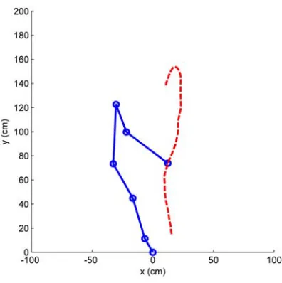
A sample trajectory is proposed. Fig. 5 shows the proposed trajectory in dashed line along with a sample robot configuration on τ =14. The proposed trajectory is broken into 33 instances of time, n=33. Each step is passed within 1/25s. The robot must traverse the predefined trajectory of length 1.61m in 1.32s.
Three other approaches in addition to our approach are applied to our sample manipulator and the predefined trajectory, [2, 4, 6]. The performance of the four approaches are compared, despite that the approaches mentioned in [2, 4, 6] have drift from the exact predefined trajectory. Fig. 6 shows the performance of the four approaches in a single task on vertical axis versus the generations on horizontal axis. Elitism operator is applied in all the 4 approaches. It is shown that within an equal number of generations, our approach reaches to a better fitness value. RNG with uniform distribution is used throughout this simulation.
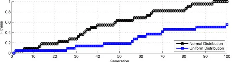
To study the role of type of RNG, ℜ, in the overall performance of our approach, two setups were considered, Table IV. Each setup ran for 100 generations. Fig. 7 shows the performance of the algorithm related to each setup. The fitness values are normalized for the best fitness value.
V. CONCLUSION
A motion planning and trajectory tracking optimization problem is solved. Genetic Algorithm (GA) is proposed as the optimization method. The introduced approach benefits from two key features. One lies on alternating the model of the manipulator from 6 degrees of rotary freedom to 4 degrees of rotary freedom and a single binary value. The other advantage of the proposed approach is the manner of data representation in each chromosome. Sigmoid function is used to infer the joints angle value. The proposed algorithm is compared with 3 other approaches in a single optimization task. It is shown that the introduced algorithm has a better performance. In addition the difference of using Random Number Generator (RNG) with uniform distribution and with normal distribution is addressed. It is shown that RNG with
[image:5.612.70.268.54.253.2]
normal distribution can achieve better results.
ACKNOWLEDGMENT
The author thanks Dr. Ahmedreza Arshi and Dr. Elham Shirzad for their suggestions and technical help.
REFERENCES
[1] A. C. Nearchou, "Solving the inverse kinematics problem of redundant robots operating in complex environments via a modified genetic algorithm," Mechanism and Machine Theory, vol. 33, pp. 273-292, 1998. [2] B. McAvoy, B. Sangolola, and Z. Szabad, "Optimal trajectory
generation for redundant planar manipulator," in IEEE International Conference on Systems, Man, and Cybernetics, Nashville, 2000, pp. 3241-3246.
[3] L. Tian and C. Collins, "Motion Planning for Redundant Manipulators Using a Floating Point Genetic Algorithm," Journal of Intelligent and Robotic Systems, vol. 38, pp. 297-312, 2003.
[4] A. A. Ata and T. R. Myo, "Optimal Point-to-Point Trajectory Tracking of Redundant Manipulators using Generalized Pattern Search," International Journal of Advanced Robotic Systems, vol. 2, pp. 239-244, 2005.
[5] Y. Davidor, "Genetic Algorithms and Robotics: A Heuristic Strategy for Optimization," World Scientific, 1991, pp. 163-168.
[6] W. M. Yun and Y. G. Xi, "Optimum motion planning in joint space for robots using genetic algorithms," Robotics and Autonomous Systems, vol. 18, pp. 373-393, 1996.
[7] A. R. Hirakawa and A. Kawamura, "Trajectory Generation for Redundant Manipulators under Optimization of Consumed Electrical Energy," in The 31st IAS Annual Meeting IAS, 1996, pp. 1626-1632. [8] Y. Nakamura, Advanced Robotics, Redundancy and Optimization.
Boston, MA, USA: Addison-Wesley Longman Publishing Co., Inc., 1990.
[9] D. E. Goldberg, Genetic Algorithm in Search, Optimization and Machine Learning: MA: Addison Wesley, 1989.
[10] J. H. Holland, Adaptation in Natural and Artificial Systems. Ann Arbor, MI: University of Michigan Press, 1975.
[11] J. J. Grefenstette, "Optimization of control parameters for genetic algorithm," IEEE Transaction on Systems, Man, Cybernetics, vol. 16, pp. 122-128, 1986.
[12] G. Rudolph, "Convergence Analysis of Canonical Genetic Algorithms," IEEE Transactions on Neural Networks, vol. 5, pp. 94-101, 1994.
[image:6.612.99.499.58.248.2]
Fig. 6. Comparison between 4 different approaches.
[image:6.612.104.498.261.367.2]