Neural Text Generation from Structured Data with Application to the Biography Domain

Neural Text Generation from Structured Data

with Application to the Biography Domain

R´emi Lebret∗

EPFL, Switzerland Facebook AI ResearchDavid Grangier Facebook AI ResearchMichael Auli

Abstract

This paper introduces a neural model for concept-to-text generation that scales to large, rich domains. It generates biographical sen-tences from fact tables on a new dataset of biographies from Wikipedia. This set is an order of magnitude larger than existing re-sources with over 700k samples and a 400k vocabulary. Our model builds on conditional neural language models for text generation. To deal with the large vocabulary, we ex-tend these models to mix a fixed vocabulary withcopy actionsthat transfer sample-specific words from the input database to the gener-ated output sentence. To deal with structured data, we allow the model to embed words differently depending on the data fields in which they occur. Our neural model signif-icantly outperforms a Templated Kneser-Ney language model by nearly 15 BLEU.

1 Introduction

Concept-to-text generation renders structured records into natural language (Reiter et al., 2000). A typical application is to generate a weather forecast based on a set of structured meteorological mea-surements. In contrast to previous work, we scale to the large and very diverse problem of generating biographies based on Wikipedia infoboxes. An infobox is a fact table describing a person, similar to a person subgraph in a knowledge base (Bollacker et al., 2008; Ferrucci, 2012). Similar generation applications include the generation of product descriptions based on a catalog of millions of items with dozens of attributes each.

Previous work experimented with datasets that contain only a few tens of thousands of records such as WEATHERGOV or the ROBOCUP dataset, while our dataset contains over 700k biographies from

∗_{R´emi performed this work while interning at Facebook.}

Wikipedia. Furthermore, these datasets have a lim-ited vocabulary of only about 350 words each, com-pared to over 400k words in our dataset.

To tackle this problem we introduce a statistical generation model conditioned on a Wikipedia in-fobox. We focus on the generation of the first sen-tence of a biography which requires the model to select among a large number of possible fields to generate an adequate output. Such diversity makes it difficult for classical count-based models to esti-mate probabilities of rare events due to data sparsity. We address this issue by parameterizing words and fields as embeddings, along with a neural language model operating on them (Bengio et al., 2003). This factorization allows us to scale to a larger number of words and fields than Liang et al. (2009), or Kim and Mooney (2010) where the number of parame-ters grows as the product of the number of words and fields.

Moreover, our approach does not restrict the re-lations between the field contents and the gener-ated text. This contrasts with less flexible strategies that assume the generation to follow either a hybrid alignment tree (Kim and Mooney, 2010), a proba-bilistic context-free grammar (Konstas and Lapata, 2013), or a tree adjoining grammar (Gyawali and Gardent, 2014).

Our model exploits structured data both globally and locally. Global conditioning summarizes all in-formation about a personality to understand high-level themes such as that the biography is about a scientist or an artist, while as local conditioning de-scribes the previously generated tokens in terms of the their relationship to the infobox. We analyze the effectiveness of each and demonstrate their comple-mentarity.

2 Related Work

Androut-sopoulos, 2007; Turner et al., 2010). Generation is divided into modular, yet highly interdependent, de-cisions: (1)content planningdefines which parts of the input fields or meaning representations should be selected; (2)sentence planningdetermines which selected fields are to be dealt with in each output sentence; and (3)surface realizationgenerates those sentences.

Data-driven approaches have been proposed to automatically learn the individual modules. One ap-proach first aligns records and sentences and then learns a content selection model (Duboue and McK-eown, 2002; Barzilay and Lapata, 2005). Hierar-chical hidden semi-Markov generative models have also been used to first determine which facts to dis-cuss and then to generate words from the predi-cates and arguments of the chosen facts (Liang et al., 2009). Sentence planning has been formulated as a supervised set partitioning problem over facts where each partition corresponds to a sentence (Barzilay and Lapata, 2006). End-to-end approaches have combined sentence planning and surface realiza-tion by using explicitly aligned sentence/meaning pairs as training data (Ratnaparkhi, 2002; Wong and Mooney, 2007; Belz, 2008; Lu and Ng, 2011). More recently, content selection and surface realization have been combined (Angeli et al., 2010; Kim and Mooney, 2010; Konstas and Lapata, 2013).

At the intersection of rule-based and statisti-cal methods, hybrid systems aim at leveraging hu-man contributed rules and corpus statistics (Langk-ilde and Knight, 1998; Soricut and Marcu, 2006; Mairesse and Walker, 2011).

Our approach is inspired by the recent success of neural language models for image captioning (Kiros et al., 2014; Karpathy and Fei-Fei, 2015; Vinyals et al., 2015; Fang et al., 2015; Xu et al., 2015), ma-chine translation (Devlin et al., 2014; Bahdanau et al., 2015; Luong et al., 2015), and modeling conver-sations and dialogues (Shang et al., 2015; Wen et al., 2015; Yao et al., 2015).

Our model is most similar to Mei et al. (2016) who use an encoder-decoder style neural network model to tackle the WEATHERGOVand ROBOCUP tasks. Their architecture relies on LSTM units and an attention mechanism which reduces scalability compared to our simpler design.

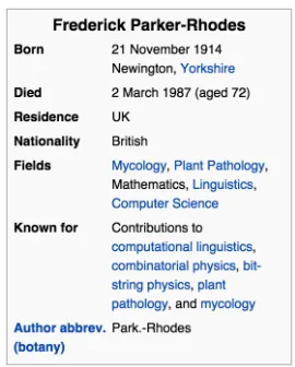
Figure 1:Wikipedia infobox of Frederick Parker-Rhodes. The introduction of his article reads: “Frederick Parker-Rhodes (21 March 1914 – 21 November 1987) was an English linguist, plant pathologist, computer scientist, mathematician, mystic, and mycologist.”.

3 Language Modeling for Constrained Sentence generation

Conditional language models are a popular choice to generate sentences. We introduce a table-conditioned language model for constraining text generation to include elements from fact tables.

3.1 Language model

Given a sentence s = w1, . . . , wT with T words from vocabulary_W, a language model estimates:

P(s) =

T

Y

t=1

P(wt|w1, . . . , wt−1). (1)

Letct = wt−(n−1), . . . , wt−1be the sequence of n₋1context words precedingwt. Ann-gram lan-guage model makes an ordernMarkov assumption,

P(s)_≈

T

Y

t=1

P(wt|ct). (2)

3.2 Language model conditioned on tables

A table is a set of field/value pairs, where values are sequences of words. We therefore propose language models that are conditioned on these pairs.

Table(gf, gw)

name John Doe birthdate 18 April 1352 birthplace Oxford UK occupation placeholder spouse Jane Doe children Johnnie Doe

input text(ct, zct)

John Doe ( 18 April 1352 ) is a

ct 13944 unk 17 37 92 25 18 12 4

zct

(name,1,2) (name,2,1) ∅ (birthd.,1,3) (birthd.,2,2) (birthd.,3,1) ∅ ∅ ∅

(spouse,2,1) (children,2,1)

output candidates(w∈ W ∪ Q)

the . . . april . . . placeholder . . . john . . . doe

w 1 . . . 92 . . . 5302 . . . 13944 . . . unk

zw

∅ (birthd.,2,2) (occupation,1,1) (name,1,2) (name,2,1) (spouse,2,1) (children,2,1)

Figure 2:Table features (right) for an example table (left);W ∪ Qis the set of all output words as defined in Section 3.3.

model. The table allows us to describe each word not only by its string (or index in the vocabulary) but also by a descriptor of its occurrence in the ta-ble. Let_Fdefine the set of all possible fieldsf. The

occurrence of a wordw in the table is described by a set of (field, position) pairs.

zw=(fi, pi) m_i=1, (3)

wherem is the number of occurrences ofw. Each pair(f, p)indicates thatwoccurs in fieldfat

posi-tionp. In this scheme, most words are described by

the empty set as they do not occur in the table. For example, the wordlinguisticsin the table of Figure 1 is described as follows:

zlinguistics ={(fields,8); (known for,4)}, (4)

assuming words are lower-cased and commas are treated as separate tokens.

Conditioning both on the field type and the po-sition within the field allows the model to encode field-specific regularities, e.g., a number token in a date field is likely followed by a month token; know-ing that the number is the first token in the date field makes this even more likely.

The (field, position) description scheme of the ta-ble does not allow to express that a token terminates a field which can be useful to capture field transi-tions. For biographies, the last token of the name field is often followed by an introduction of the birth date like ‘(’ or ‘was born’. We hence extend our de-scriptor to a triplet that includes the position of the

token counted from the end of the field:

zw=(fi, p+i , p−i ) m

i=1, (5)

where our example becomes:

zlinguistics={(fields,8,4); (known for,4,13)}.

We extend Equation 2 to use the above informa-tion as addiinforma-tional condiinforma-tioning context when gener-ating a sentences:

P(s_|z) =

T

Y

t=1

P(wt|ct, zct), (6)

wherezct = zwt−(n−1), . . . , zwt−1 are referred to as the local conditioning variables since they describe the local context (previous word) relations with the table.

Global conditioningrefers to information from all tokens and fields of the table, regardless whether they appear in the previous generated words or not. The set of fields available in a table often impacts the structure of the generation. For biographies, the fields used to describe a politician are different from the ones for an actor or an athlete. We introduce global conditioning on the available fieldsgf as

P(s_|z, gf) = T

Y

t=1

P(wt|ct, zct, gf). (7)

words occurring in the table is introduced:

P(s_|z, gf, gw) = T

Y

t=1

P(wt|ct, zct, gf, gw). (8)

Tokens provide information complementary to fields. For example, it may be hard to distinguish a basketball player from a hockey player by looking only at the field names, e.g. teams, league, position, weight and height, etc. However the actual field tokens such as team names, league name, player’s position can help the model to give a better pre-diction. Here, gf ∈ {0,1}F and gw ∈ {0,1}W are binary indicators over fixed field and word vocabularies.

Figure 2 illustrates the model with a schematic ex-ample. For predicting the next wordwtafter a given contextct, the language model is conditioned on sets of triplets for each word occurring in the tablezct,

along with all fields and words from this table.

3.3 Copy actions

So far we extended the model conditioning with fea-tures derived from the fact table. We now turn to using table information when scoring output words. In particular, sentences which express facts from a given table often copy words from the table. We therefore extend our model to also score special field tokens such as name 1 or name 2 which are sub-sequently added to the score of the corresponding words from the field value.

Our model reads a table and defines an output do-mainW ∪Q.Qdefines all tokens in the table, which might include out of vocabulary words (∈ W/ ). For instancePark-Rhodesin Figure 1 is not in_W. How-ever,Park-Rhodeswill be included in_Qasname 2 (since it is the second token of the name field) which allows our model to generate it. This mechanism is inspired by recent work on attention based word copying for neural machine translation (Luong et al., 2015) as well as delexicalization for neural dialog systems (Wen et al., 2015). It also builds upon older work such as class-based language models for dialog systems (Oh and Rudnicky, 2000).

4 A Neural Language Model Approach A feed-forward neural language model (NLM) es-timates P(wt|ct) with a parametric function φθ

(Equation 1), whereθrefers to all learnable

param-eters of the network. This function is a composition of simple differentiable functions orlayers.

4.1 Mathematical notations and layers

We denote matrices as bold upper case letters (X, Y,Z), and vectors as bold lower-case letters (a,b,

c). Ai represents the ith row of matrix A. When

A is a 3-d matrix, then Ai,j represents the vector of theith first dimension andjth second dimension.

Unless otherwise stated, vectors are assumed to be column vectors. We use [v1;v2] to denote vector

concatenation. Next, we introduce the notation for the different layers used in our approach.

Embedding layer. Given a parameter matrix

X _{∈ R}N×d_{, theembedding layeris a lookup table} that performs an array indexing operation:

ψ_X(xi) =Xi ∈Rd, (9)

whereXi corresponds to the embedding of the ele-mentxiat rowi. WhenXis a 3-d matrix, the lookup table takes two arguments:

ψ_X(xi, xj) =Xi,j ∈Rd, (10)

where Xi,j corresponds to the embedding of the pair (xi, xj) at index (i, j). The lookup table op-eration can be applied for a sequence of elements

s=x1, . . . , xT. A common approach is to concate-nate all resulting embeddings:

ψ_X(s) =ψ_X(x1);. . .;ψ_X(xT)∈RT×d. (11)

Linear layer. This layer applies a linear trans-formation to its inputsx_∈Rn_:

γ_θ(x) =Wx+b (12)

where θ = _{W,b_} are the trainable parameters

with W _{∈ R}m×n _{being the weight matrix, and}

b∈Rm_{is the bias term.}

Softmax layer. Given a context input ct, the final layer outputs a score for each wordwt ∈ W,

φ_θ(ct) ∈ R|W|. The probability distribution is ob-tained by applying the softmax activation function:

P(wt =w|ct) =

exp(φ_θ(ct, w))

P|W|

i=1exp(φθ(ct, wi))

4.2 Embeddings as inputs

A key aspect of neural language models is the use of word embeddings. Similar words tend to have similar embeddings and thus share latent features. The probability estimates of those models are smooth functions of these embeddings, and a small change in the features results in a small change in the probability estimates (Bengio et al., 2003). Therefore, neural language models can achieve better generalization for unseen n-grams. Next, we show how we map fact tables to continuous space in similar spirit.

Word embeddings. Formally, the embedding layer maps each context word index to a continuous

d-dimensional vector. It relies on a parameter

ma-trixE _∈ R|W|×d to convert the inputct inton−1 vectors of dimensiond:

ψ_E(ct) =ψE(wt−(n−1));. . .;ψE(wt−1). (14) E can be initialized randomly or with pre-trained

word embeddings.

Table embeddings. As described in Section 3.2, the language model is conditioned on elements from the table. Embedding matrices are therefore defined to model both local and global conditioning infor-mation. For local conditioning, we denote the maxi-mum length of a sequence of words asl. Each field

fj ∈ F is associated with 2 ×l vectors of d di-mensions, the firstlof those vectors embed all

pos-sible starting positions1, . . . , l, and the remainingl

vectors embed ending positions. This results in two parameter matrices Z = {Z+,Z−} ∈ R|F|×l×d_. For a given triplet (fj, p+_i , p−_i ), ψZ+(fj, p+_i ) and

ψ_Z−(fj, p−i )refer to the embedding vectors of the start and end position for fieldfj, respectively.

Finally, global conditioning uses two parame-ter matrices Gf _{∈ R}|F|×g _{and G}w _{∈ R}|W|×g_.

ψ_Gf(fj) maps a table field fj into a vector of dimensiong, whileψ_Gw(wt)maps a wordwt into a vector of the same dimension. In general, Gw

shares its parameters withE, providedd=g.

Aggregating embeddings.We represent each oc-curence of a word w as a triplet (field, start, end)

where we have embeddings for the start and end po-sition as described above. Often times a particular wordw occurs multiple times in a table, e.g.,

‘lin-guistics’ has two instances in Figure 1. In this case, we perform a component-wise max over the start embeddings of all instances ofw to obtain the best

features across all occurrences ofw. We do the same for end position embeddings:

ψ_Z(zwt) =

h

maxψ_Z+(f_j, p+_i ),∀(f_j, p+_i , p−_i )∈z_wt ; maxψ_Z−(fj, p−_i ),∀(fj, p+_i , p−_i )∈zwt

i (15)

A special no-field embedding is assigned towtwhen the word is not associated to any fields. An embed-dingψ_Z(zct)for encoding the local conditioning of

the inputctis obtained by concatenation.

For global conditioning, we defineFq_{⊂ F as the} set of all the fields in a given tableq, andQas the set of all words inq. We also perform max aggregation.

This yields the vectors

ψ_Gf(g_f) = maxψ_Gf(f_j),∀f_j∈ Fq , (16)

and

ψ_Gw(g_w) = maxψ_Gw(w_t),∀w_t ∈ Q . (17)

The final embedding which encodes the context in-put with conditioning is then the concatenation of these vectors:

ψ_α1(ct, zct, gf, gw) =

ψ_E(ct);ψZ(zct);

ψ_Gf(g_f);ψ_Gw(gw)∈Rd

1

, (18)

withα1 = {E,Z+,Z−,Gf,Gw} andd1 = (n−

1)×(3×d) + (2×g). For simplification purpose,

we define the context inputx = _{ct, zct, gf, gw}in

the following equations. This context embedding is mapped to a latent context representation using a lin-ear operation followed by a hyperbolic tangent:

h(x) = tanhγ_α2 ψ_α1(x)∈Rnhu, (19)

where α2 = {W2,b2}, withW2 ∈ Rnhu×d

1 and

b2∈Rnhu.

4.3 In-vocabulary outputs

The hidden representation of the context then goes to another linear layer to produce a real value score for each word in the vocabulary:

whereα3 = {W3,b3}, withW3 ∈ R|W|×nhuand b3 ∈R|W|, andα={α1, α2, α3}.

4.4 Mixing outputs for better copying

Section 3.3 explains that each wordwfrom the table is also associated withzw, the set of fields in which it occurs, along with the position in that field. Simi-lar to local conditioning, we represent each field and position pair(fj, pi)with an embeddingψF(fj, pi), where F _∈ R|F|×l×d_{. These embeddings are then} projected into the same space as the latent represen-tation of context inputh(x)∈Rnhu_{. Using the max}

operation over the embedding dimension, each word is finally embedded into a unique vector:

q(w) = max

tanhγ_β ψ_F(fj, pi),∀(fj, pi)∈zw , (21)

where β = _{W4,b4} with W4 ∈ Rnhu×d, and b4 ∈ Rnhu. A dot product with the context vector

produces a score for each wordwin the table,

φQ_β(x, w) =h(x)_·q(w). (22) Each wordw _{∈ W ∪ Q}receives a final score by summing the vocabulary score and the field score:

φθ(x, w) =φWα (x, w) +φQβ(x, w), (23) withθ = {α, β}, and where φQ_β(x, w) = 0 when w /∈ Q. The softmax function then maps the scores to a distribution over_{W ∪ Q},

logP(w_|x) =φθ(x, w)−log

X

w0_∈W∪Q

expφθ(x, w0).

4.5 Training

The neural language model is trained to minimize the negative log-likelihood of a training sentences

with stochastic gradient descent (SGD; LeCun et al. 2012) :

Lθ(s) =− T

X

t=1

logP(wt|ct, zct, gf, gw). (24)

5 Experiments

Our neural network model (Section 4) is designed to generate sentences from tables for large-scale prob-lems, where a diverse set of sentence types need to be generated. Biographies are therefore a good

framework to evaluate our model, with Wikipedia offering a large and diverse dataset.

5.1 Biography dataset

We introduce a new dataset for text generation, WIKIBIO, a corpus of 728,321 articles from En-glish Wikipedia (Sep 2015). It comprises all biogra-phy articles listed by WikiProject Biograbiogra-phy1_which

also have a table (infobox). We extract and tok-enize the first sentence of each article with Stanford CoreNLP (Manning et al., 2014). All numbers are mapped to a special token, except for years which are mapped to different special token. Field values from tables are similarly tokenized. All tokens are lower-cased. Table 2 summarizes the dataset statis-tics: on average, the first sentence is twice as short as the table (26.1 vs 53.1 tokens), about a third of the sentence tokens (9.5) also occur in the table. The final corpus has been divided into three sub-parts to provide training (80%), validation (10%) and test sets (10%). The dataset is available for download2_.

5.2 Baseline

Our baseline is an interpolated Kneser-Ney (KN) language model and we use the KenLM toolkit to train 5-gram models without pruning (Heafield et al., 2013). We also learn a KN language model over templates. For that purpose, we re-place the words occurring in both the table and the training sentences with a special token reflect-ing its table descriptor zw (Equation 3). The in-troduction section of the table in Figure 1 looks as follows under this scheme: “name 1 name 2 ( birthdate 1 birthdate 2 birthdate 3 – deathdate 1 deathdate 2 deathdate 3 ) was an english linguist , fields 3 pathologist , fields 10scientist , mathematician , mystic and mycologist .” During inference, the decoder is con-strained to emit words from the regular vocabulary or special tokens occurring in the input table. When picking a special token we copy the corresponding word from the table.

5.3 Training setup

For our neural models, we train 11-gram language models (n= 11) with a learning rate set to0.0025.

1_{https://en.wikipedia.org/wiki/} Wikipedia:WikiProject_Biography

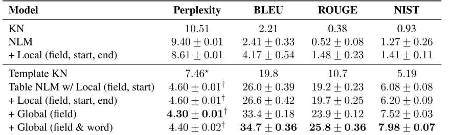
Model Perplexity BLEU ROUGE NIST

KN 10.51 2.21 0.38 0.93

NLM 9.40 +₋0.01 2.41 +₋0.33 0.52 +₋0.08 1.27 +₋0.26

+ Local (field, start, end) 8.61 +₋0.01 4.17 +₋0.54 1.48 +₋0.23 1.41 +₋0.11

Template KN 7.46? 19.8 10.7 5.19

Table NLM w/ Local (field, start) 4.60 +₋0.01† _{26.0 +}

−0.39 19.2 +−0.23 6.08 +−0.08

+ Local (field, start, end) 4.60 +₋0.01† 26.6 +₋0.42 19.7 +₋0.25 6.20 +₋0.09

+ Global (field) 4.30+₋0.01† 33.4 +₋0.18 23.9 +₋0.12 7.52 +₋0.03

+ Global (field & word) 4.40 +₋0.02† 34.7+₋0.36 25.8+₋0.36 7.98+₋0.07

Table 1:BLEU, ROUGE, NIST and perplexity without copy actions (first three rows) and with copy actions (last five rows). For neural models we report “mean+₋standard deviation” for five training runs with different initialization. Decoding beam width is 5. Perplexities marked with?_and†_{are not directly comparable as the output vocabularies differ slightly.}

Mean Percentile

5% 95% # tokens per sentence 26.1 13 46 # tokens per table 53.1 20 108 # table tokens per sent. 9.5 3 19 # fields per table 19.7 9 36

Table 2:Dataset statistics

Parameter Value

# word types _|W| = 20,000

# field types |F| = 1,740

Max. # tokens in a field l = 10

word/field embedding size d = 64

global embedding size g = 128

# hidden units nhu = 256

Table 3:Model Hyperparameters

Table 3 describes the other hyper-parameters. We include all fields occurring at least 100 times in the training data in F, the set of fields. We include the20,000 most frequent words in the vocabulary.

The other hyperparameters are set through valida-tion, maximizing BLEU over a validation subset of

1,000 sentences. Similarly, early stopping is ap-plied: training ends when BLEU stops improving on the same validation subset. One should note that the maximum number of tokens in a field l = 10

means that we encode only10positions: for longer

field values the final tokens are not dropped but their position is capped to10. We initialize the word

em-beddingsW from Hellinger PCA computed over the

set of training biographies. This representation has

shown to be helpful for various applications (Lebret and Collobert, 2014).

5.4 Evaluation metrics

We use different metrics to evaluate our models. Performance is first evaluated in terms of perplex-ity which is the standard metric for language mod-eling. Generation quality is assessed automatically with BLEU-4, ROUGE-4 (F-measure) and NIST-43_{(Belz and Reiter, 2006).}

6 Results

This section describes our results and discusses the impact of the different conditioning variables.

6.1 The more, the better

The results (Table 1) show that more conditioning information helps to improve the performance of our models. The generation metrics BLEU, ROUGE and NIST all gives the same performance ordering over models. We first discuss models without copy actions (the first three results) and then discuss mod-els with copy actions (the remaining results). Note that the factorization of our models results in three different output domains which makes perplexity comparisons less straightforward: models without copy actions operate over a fixed vocabulary. Tem-plate KN adds a fixed set of field/position pairs to this vocabulary while Table NLM models a variable setQdepending on the input table, see Section 3.3.

Without copy actions.In terms of perplexity the (i) neural language model (NLM) is slightly better 3_{We rely on standard software, NIST mteval-v13a.pl (for}

than an interpolated KN language model, and (ii) adding local conditioning on the field start and end position further improves accuracy. Generation met-rics are generally very low but there is a clear im-provement when using local conditioning since it al-lows to learn transitions between fields by linking previous predictions to the table unlike KN or plain NLM.

With copy actions. For experiments with copy actions we use the full local conditioning (Equa-tion 4) in the neural language models. BLEU, ROUGE and NIST all improves when moving from Template KN to Table NLM and more features suc-cessively improve accuracy. Global conditioning on the fields improves the model by over 7 BLEU and adding words gives an additional 1.3 BLEU. This is a total improvement of nearly 15 BLEU over the Template Kneser-Ney baseline. Similar observa-tions are made for ROUGE +15 and NIST +2.8.

●

● ● ●

● ●

● ●● ● ● ● ●

100 200 500 1000 2000

15

20

25

30

35

40

45

time in ms

BLEU

● ●●

● ●● ● ●● ●

● ●

●

1

2 3

4 56 _{8 10 15 2025}

1

3 4 5 6 7 810

15 _{20 25}

●

Template KN Table NLM beam size

Figure 3: Comparison between our best model (Table NLM) and the baseline (Template KN) for different beam sizes. The x-axis is the average timing (in milliseconds) for generating one sentence. The y-axis is the BLEU score. All results are mea-sured on a subset of 1,000 samples of the validation set.

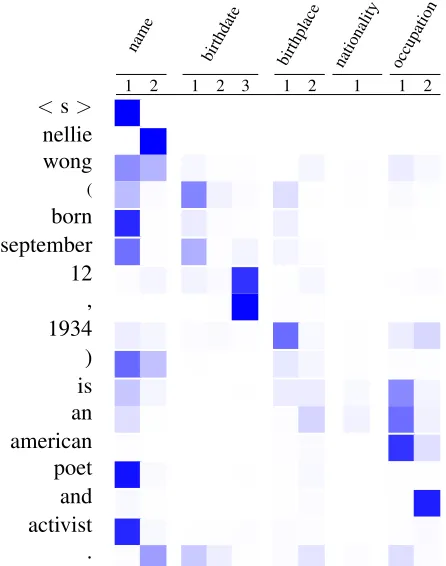
6.2 Attention mechanism

Our model implements attention over input table fields. For each wordw in the table, Equation (23)

takes the language model scoreφW_ct and adds a bias φQ_ct. The bias is the dot-product between a

represen-tation of the table field in whichwoccurs and a

rep-resentation of the context, Equation (22) that sum-marizes the previously generated fields and words.

name _birthdate

birthplace nationality occupation

1 2 1 2 3 1 2 1 1 2

<s>

nellie wong ( born september 12 , 1934 ) is an american poet and activist .

Figure 4: Visualization of attention scores for Nellie Wong’s Wikipedia infobox. Each row represents the probability distri-bution over (field, position) pairs given the previous words (i.e. the words heading the preceding rows as well as the current row). Darker colors depict higher probabilities.

Figure 4 shows that this mechanism adds a large bias to continue a field if it has not generated all tokens from the table, e.g., it emits the word oc-curring inname 2after generating name 1. It also nicely handles transitions between field types, e.g., the model adds a large bias to the words occurring in theoccupationfield after emitting thebirthdate.

6.3 Sentence decoding

We use a standard beam search to explore a larger set of sentences compared to simple greedy search. This allows us to exploreKtimes more paths which

comes at a linear increase in the number of forward computation steps for our language model. We com-pare various beam settings for the baseline Template KN and our Table NLM (Figure 3). The best vali-dation BLEU can be obtained with a beam size of

K = 5. Our model is also several times faster than

the baseline, requiring only about 200 ms per sen-tence withK = 5. Beam search generates many

Model Generated Sentence

Reference frederick parker-rhodes (21 march 1914 – 21 november 1987) was an english linguist, plant_{pathologist, computer scientist, mathematician, mystic, and mycologist.}

Baseline

(Template KN) frederick parker-rhodes ( born november 21 , 1914 – march 2 , 1987 ) was an english cricketer.

Table NLM +Local (field, start)

frederick parker-rhodes ( 21 november 1914 – 2 march 1987 ) was an australian rules foot-baller who played with carlton in the victorian football league ( vfl ) during the XXXXs and XXXXs .

+ Global (field) frederick parker-rhodes ( 21 november 1914 – 2 march 1987 ) was an english mycology and_{plant pathology , mathematics at the university of uk .}

+ Global

(field, word) frederick parker-rhodes ( 21 november 1914 – 2 march 1987 ) was a british computer scientist, best known for his contributions to computational linguistics .

Table 4: First sentence from the current Wikipedia article about Frederick Parker-Rhodes and the sentences generated from the three versions of our table-conditioned neural language model (Table NLM) using the Wikipedia infobox seen in Figure 1.

random memory accesses; while neural models per-form scoring through matrix-matrix products, an op-eration which is more local and can be performed in a block parallel manner where modern graphic pro-cessors shine (Kindratenko, 2014).

6.4 Qualitative analysis

Table 4 shows generations for different variants of our model based on the Wikipedia table in Figure 1. First of all, comparing the reference to the fact table reveals that our training data is not perfect. The birth month mentioned in the fact table and the first sen-tence of the Wikipedia article are different; this may have been introduced by one contributor editing the article and not keeping the information consistent.

All three versions of our model correctly generate the beginning of the sentence by copying the name, the birth date and the death date from the table. The model correctly uses the past tense since the death date in the table indicates that the person has passed away. Frederick Parker-Rhodes was a scientist, but this occupation is not directly mentioned in the table. The model without global conditioning can there-fore not predict the right occupation, and it contin-ues the generation with the most common occupa-tion (in Wikipedia) for a person who has died. In contrast, the global conditioning over the fields helps the model to understand that this person was indeed a scientist. However, it is only with the global con-ditioning on the words that the model can infer the correct occupation, i.e.,computer scientist.

7 Conclusions

We have shown that our model can generate flu-ent descriptions of arbitrary people based on struc-tured data. Local and global conditioning improves our model by a large margin and we outperform a Kneser-Ney language model by nearly 15 BLEU. Our task uses an order of magnitude more data than previous work and has a vocabulary that is three or-ders of magnitude larger.

In this paper, we have only focused on generating the first sentence and we will tackle the generation of longer biographies in future work. Also, the encod-ing of field values can be improved. Currently, we only attach the field type and token position to each word type and perform a max-pooling for local con-ditioning. One could leverage a richer representation by learning an encoder conditioned on the field type, e.g. a recurrent encoder or a convolutional encoder with different pooling strategies.

References

G. Angeli, P. Liang, and D. Klein. 2010. A simple domain-independent probabilistic approach to genera-tion. InProceedings of the 2010 Conference on Empir-ical Methods in Natural Language Processing, pages 502–512. Association for Computational Linguistics. D. Bahdanau, K. Cho, and Y. Bengio. 2015. Neural

ma-chine translation by jointly learning to align and trans-late. InInternational Conference on Learning Repre-sentations.

R. Barzilay and M. Lapata. 2005. Collective content se-lection for concept-to-text generation. InProceedings of the conference on Human Language Technology and Empirical Methods in Natural Language Processing, pages 331–338.

R. Barzilay and M. Lapata. 2006. Aggregation via set partitioning for natural language generation. In Pro-ceedings of the main conference on Human Language Technology Conference of the North American Chapter of the Association of Computational Linguistics, pages 359–366. Association for Computational Linguistics. A. Belz and E. Reiter. 2006. Comparing automatic and

human evaluation of nlg systems. InIn Proc. EACL06, pages 313–320.

A. Belz. 2008. Automatic generation of weather forecast texts using comprehensive probabilistic generation-space models. Natural Language Engineering, 14(04):431–455.

Y. Bengio, R. Ducharme, P. Vincent, and C. Jauvin. 2003. A neural probabilistic language model.Journal of Ma-chine Learning Research, 3:1137–1155.

K. Bollacker, C. Evans, P. Paritosh, T. Sturge, and J. Tay-lor. 2008. Freebase: a collaboratively created graph database for structuring human knowledge. In Inter-national Conference on Management of Data, pages 1247–1250. ACM.

R. Dale, S. Geldof, and J.-P. Prost. 2003. Coral: Us-ing natural language generation for navigational as-sistance. In Proceedings of the 26th Australasian computer science conference-Volume 16, pages 35–44. Australian Computer Society, Inc.

J. Devlin, R. Zbib, Z. Huang, T. Lamar, R. Schwartz, and J. Makhoul. 2014. Fast and robust neural network joint models for statistical machine translation. In Pro-ceedings of the 52nd Annual Meeting of the Associa-tion for ComputaAssocia-tional Linguistics, volume 1, pages 1370–1380.

P. A. Duboue and K. R. McKeown. 2002. Content planner construction via evolutionary algorithms and a corpus-based fitness function. InProceedings of INLG 2002, pages 89–96.

H. Fang, S. Gupta, F. Iandola, R. K. Srivastava, L. Deng, P. Dollar, J. Gao, X. He, M. Mitchell, J. C. Platt, L. C.

Zitnick, and G. Zweig. 2015. From captions to visual concepts and back. InThe IEEE Conference on Com-puter Vision and Pattern Recognition (CVPR), June. D. Ferrucci. 2012. Introduction to this is watson. IBM

Journal of Research and Development, 56(3.4):1–1. D. Galanis and I. Androutsopoulos. 2007. Generating

multilingual descriptions from linguistically annotated owl ontologies: the naturalowl system. In Proceed-ings of the Eleventh European Workshop on Natural Language Generation, pages 143–146. Association for Computational Linguistics.

N. Green. 2006. Generation of biomedical arguments for lay readers. InProceedings of the Fourth International Natural Language Generation Conference, pages 114– 121. Association for Computational Linguistics. B. Gyawali and C. Gardent. 2014. Surface realisation

from knowledge-bases. InProc. of ACL.

K. Heafield, I. Pouzyrevsky, J. H. Clark, and P. Koehn. 2013. Scalable modified Kneser-Ney language model estimation. In Proceedings of the 51st Annual Meet-ing of the Association for Computational LMeet-inguistics, pages 690–696, Sofia, Bulgaria, August.

A. Karpathy and L. Fei-Fei. 2015. Deep visual-semantic alignments for generating image descriptions. InThe IEEE Conference on Computer Vision and Pattern Recognition (CVPR), June.

J. Kim and R. J. Mooney. 2010. Generative alignment and semantic parsing for learning from ambiguous su-pervision. In Proceedings of the 23rd International Conference on Computational Linguistics: Posters, pages 543–551. Association for Computational Lin-guistics.

V. Kindratenko. 2014. Numerical Computations with GPUs. Springer.

R. Kiros, R. Salakhutdinov, and R. S. Zemel. 2014. Unifying visual-semantic embeddings with multi-modal neural language models. arXiv preprint arXiv:1411.2539.

I. Konstas and M. Lapata. 2013. A global model for concept-to-text generation. J. Artif. Int. Res., 48(1):305–346, October.

I. Langkilde and K. Knight. 1998. Generation that ex-ploits corpus-based statistical knowledge. In Proc. ACL, pages 704–710.

R. Lebret and R. Collobert. 2014. Word embeddings through hellinger pca. InProceedings of the 14th Con-ference of the European Chapter of the Association for Computational Linguistics, pages 482–490, Gothen-burg, Sweden, April. Association for Computational Linguistics.

P. Liang, M. I. Jordan, and D. Klein. 2009. Learning semantic correspondences with less supervision. In

Proceedings of the Joint Conference of the 47th An-nual Meeting of the ACL and the 4th International Joint Conference on Natural Language Processing of the AFNLP: Volume 1-Volume 1, pages 91–99. Associ-ation for ComputAssoci-ational Linguistics.

W. Lu and H. T. Ng. 2011. A probabilistic forest-to-string model for language generation from typed lambda calculus expressions. In Proceedings of the Conference on Empirical Methods in Natural Lan-guage Processing, pages 1611–1622. Association for Computational Linguistics.

M.-T. Luong, I. Sutskever, Q. V Le, O. Vinyals, and W. Zaremba. 2015. Addressing the rare word prob-lem in neural machine translation. InProc. ACL, pages 11–19.

F. Mairesse and M. Walker. 2011. Controlling user per-ceptions of linguistic style: Trainable generation of personality traits.Comput. Linguist., 37(3):455–488. C. D. Manning, M. Surdeanu, J. Bauer, J. Finkel, S. J.

Bethard, and D. McClosky. 2014. The Stanford CoreNLP natural language processing toolkit. In As-sociation for Computational Linguistics (ACL) System Demonstrations, pages 55–60.

H. Mei, M. Bansal, and M. R. Walter. 2016. What to talk about and how? selective generation using lstms with coarse-to-fine alignment. InProceedings of Hu-man Language Technologies: The 2016 Annual Con-ference of the North American Chapter of the Associa-tion for ComputaAssocia-tional Linguistics.

A. Oh and A. Rudnicky. 2000. Stochastic language gen-eration for spoken dialogue systems. InANLP/NAACL Workshop on Conversational Systems, pages 27–32. A. Ratnaparkhi. 2002. Trainable approaches to

sur-face natural language generation and their application to conversational dialog systems. Computer Speech & Language, 16(3):435–455.

E. Reiter, R. Dale, and Z. Feng. 2000. Building natural language generation systems, volume 33. MIT Press. E. Reiter, S. Sripada, J. Hunter, J. Yu, and I. Davy. 2005.

Choosing words in computer-generated weather fore-casts.Artificial Intelligence, 167(1):137–169.

L. Shang, Z. Lu, and H. Li. 2015. Neural responding machine for short-text conversation. arXiv preprint arXiv:1503.02364.

Radu Soricut and Daniel Marcu. 2006. Stochastic lan-guage generation using widl-expressions and its appli-cation in machine translation and summarization. In

Proc. ACL, pages 1105–1112.

R. Turner, S. Sripada, and E. Reiter. 2010. Generating approximate geographic descriptions. In Empirical methods in natural language generation, pages 121– 140. Springer.

O. Vinyals, A. Toshev, S. Bengio, and D. Erhan. 2015. Show and tell: A neural image caption generator. In

The IEEE Conference on Computer Vision and Pattern Recognition (CVPR), June.

T. Wen, M. Gasic, N. Mrkˇsi´c, P. Su, D. Vandyke, and S. Young. 2015. Semantically conditioned lstm-based natural language generation for spoken dialogue systems. In Proceedings of the 2015 Conference on Empirical Methods in Natural Language Processing, pages 1711–1721, Lisbon, Portugal, September. Asso-ciation for Computational Linguistics.

Y. W. Wong and R. J. Mooney. 2007. Generation by inverting a semantic parser that uses statistical machine translation. InHLT-NAACL, pages 172–179.

K. Xu, J. Ba, R. Kiros, A. Courville, R. Salakhutdinov, R. Zemel, and Y. Bengio. 2015. Show, attend and tell: Neural image caption generation with visual attention. InProceedings of The 32nd International Conference on Machine Learning, volume 37, July.