University of Warwick institutional repository:
http://go.warwick.ac.uk/wrap
A Thesis Submitted for the Degree of PhD at the University of Warwick
http://go.warwick.ac.uk/wrap/77583
This thesis is made available online and is protected by original copyright.
Please scroll down to view the document itself.
Short-Pulse Laser Interactions with High Density
Plasma
by
Martin Ramsay
Thesis
Submitted to the University of Warwick
for the degree of
Doctor of Philosophy
Department of Physics
Contents
List of Tables v
List of Figures vi
Acknowledgments ix
Declarations x
Abstract xi
Abbreviations xii
Chapter 1 Introduction 1
1.1 Overview . . . 2
1.2 Basic plasma physics . . . 3
1.2.1 Plasma equations of motion . . . 3
1.2.2 Ohm’s law . . . 6
1.2.3 Debye length . . . 9
1.2.4 Plasma frequency . . . 10
1.2.5 Plasma dispersion relation . . . 11
1.2.6 Critical density . . . 13
1.3 High power lasers . . . 14
1.3.1 ‘Long-pulse’ lasers . . . 14
1.3.2 ‘Short-pulse’ lasers . . . 14
1.4 Short-pulse laser absorption . . . 15
1.4.1 Inverse bremsstrahlung . . . 16
1.4.2 Resonance absorption . . . 16
1.4.3 Vacuum heating . . . 17
1.4.4 Ponderomotive acceleration . . . 17
1.4.6 Other important processes . . . 18
1.5 Energy transport . . . 19
1.5.1 Return current generation . . . 19
1.5.2 Ohmic heating . . . 19
1.5.3 Filamentation . . . 20
1.5.4 X-ray emission . . . 20
1.6 Summary of short-pulse laser interactions . . . 21
1.7 Short-pulse laser applications . . . 22
1.7.1 Material heating . . . 22
1.7.2 X-ray sources . . . 22
1.7.3 Electron acceleration . . . 22
1.7.4 Proton acceleration . . . 23
1.7.5 Fast ignition . . . 23
1.8 Overview of plasma modelling . . . 24
1.8.1 Fluid models . . . 25
1.8.2 Kinetic models . . . 26
1.8.3 Hybrid models . . . 26
1.8.4 Summary of plasma models . . . 27
Chapter 2 Overview of the EPOCH PIC code 28 2.1 Particle-in-cell codes . . . 28
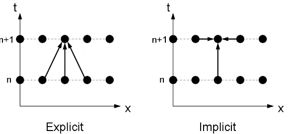
2.1.1 Explicit vs implicit schemes . . . 29
2.2 Particle propagation . . . 30
2.2.1 Particle shapes . . . 32
2.2.2 Current density calculation . . . 33
2.3 Field propagation . . . 34
2.4 Boundary conditions . . . 37
2.5 The laser package . . . 39
2.6 The limits of PIC . . . 40
2.6.1 Grid resolution . . . 41
2.6.2 Particle resolution . . . 42
2.6.3 Time-step constraints . . . 42
2.7 PIC summary . . . 44
2.8 Implementing short-range collisions inEPOCH. . . 44
2.8.1 Introduction . . . 44
2.8.2 Cumulative relativistic scattering of binary particle pairs . . . 45
2.8.4 Test problems . . . 49
Chapter 3 An Ohmic field solver for high density PIC simulations 53 3.1 Introduction . . . 53
3.2 The high density algorithm . . . 54
3.2.1 Electric field calculation . . . 54
3.2.2 Identifying particle species . . . 59
3.2.3 Multiple electron/ion species . . . 61
3.2.4 Magnetic field update . . . 61
3.2.5 Particle position and velocity update . . . 61
3.3 Implications for PIC modelling . . . 62
Chapter 4 Preliminary testing and comparisons 63 4.1 Introduction . . . 63
4.1.1 THOR summary . . . 64
4.2 Monoenergetic beam . . . 64
4.3 Diffusion . . . 66
4.4 Laser-plasma interaction . . . 68
4.4.1 1D . . . 68
4.4.2 2D . . . 69
4.5 Run times and self-heating rates . . . 70
4.6 Summary . . . 72
Chapter 5 The effect of high density transport phenomena on the TNSA process 74 5.1 Introduction . . . 74
5.2 Simulation setup . . . 75
5.3 EPOCH/EPOCH-C/EPOCH-H comparison . . . 77
5.3.1 Proton energy spectra . . . 77
5.4 Imprinting of fast electron transport effects . . . 79
5.4.1 Control of proton beam filamentation via target morphology . . 81
5.4.2 Fast electron filamentation . . . 82
5.5 Discussion . . . 86
Chapter 6 Return current heating of solid density targets 88 6.1 Modelling material heating . . . 88
6.2 Simulation parameters . . . 89
6.2.2 THOR . . . 90
6.3 Material heating comparison . . . 91
6.4 Line emission comparison . . . 95
6.5 Magnetic fields at layer interface . . . 98
6.6 Summary and discussion . . . 99
Chapter 7 Summary 102 7.1 Background . . . 102
7.2 The high density algorithm . . . 104
7.3 Effect of high density transport phenomena on proton acceleration . . . 106
7.4 Heating of solid density matter . . . 108
7.5 Future work . . . 108
7.6 Implications for further short-pulse modelling . . . 109
Appendix A Derivation of Fokker-Planck equation 111 A.1 The Landau equation . . . 113
Appendix B Derivation of radiating boundary conditions 114 Appendix C Derivation of collision parameters 117 C.1 Collision frequency . . . 117
List of Tables
3.1 Tabulated values of the Braginskii electrical resistivity coefficient. . . . 56
4.1 Computational expense and electron heating rate associated with various
versions of EPOCHfor the case of a simple, uniform system. . . 70 5.1 Tabulated values of the average temperatures in the range15µm< x <
25µmfrom figure 5.3. . . 79
5.2 Values, for various target widths (w), of the characteristic distance (λf)
between filaments in the spatial distribution of protons recorded passing
List of Figures
1.1 The plasma dispersion relations (left) and refractive indices (right) for
electromagnetic waves in a cold plasma . . . 12
1.2 The reflectivity of a plasma as a function of its electron density . . . 13
1.3 Diagrammatic representation of the fast ignition concept . . . 24
1.4 Visual representation of the disparate time-scales involved in short-pulse laser interactions . . . 25
2.1 Diagrammatic representation of the dependencies for explicit and implicit methods . . . 30
2.2 Diagrammatic representation of zeroth-order particle weighting . . . 33
2.3 Diagrammatic representation of first-order particle weighting . . . 34
2.4 An example of the 3D Yee mesh for the FDTD method . . . 35
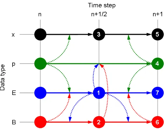
2.5 Diagram to illustrate how particle and field variables are used to update each other during a time-step . . . 37
2.6 The dispersion relation on a discrete mesh . . . 43
2.7 Diagram to illustrate the scattering angles associated with binary particle collisions . . . 47
2.8 Results of a collision algorithm test problem aiming to reproduce Spitzer conductivity . . . 50
2.9 Results of a collision algorithm test problem aiming to reproduce thermal conduction . . . 51
2.10 Demonstration of the need for high particle resolution in ensuring accurate modelling of collisional phenomena . . . 52
4.1 Results of the 1D monoenergetic beam test problem . . . 65
4.2 Results of the 1D monoenergetic beam test problem . . . 66
4.4 Comparison of theEPOCH-C andEPOCH-H background electron temper-atures in the 1D LPI test problem . . . 68 4.5 Lineout of the background electron temperatures from the 2D LPI test
problem . . . 69
4.6 Average electron temperature as a function of time, demonstrating the rate of numerical heating for theEPOCH-CandEPOCH-Hsimulations listed in table 4.1. . . 71
5.1 Lineouts of the initial electron and ion densities for the EPOCH-H and solid densityEPOCHTNSA simulations. . . 76 5.2 Time-integrated proton energy spectra. . . 77
5.3 Lineouts of the background electron temperature and total electron densities from TNSA simulations aftert= 2.0 ps. . . 78
5.4 Number of protons recorded by the probes as functions of position and
direction of motion . . . 80 5.5 Fast electron and proton number density demonstrating imprinting of
fast electron filamentation onto the accelerated proton population . . . 81 5.6 Fourier transform of the spatial distribution of protons recorded by the
particle probes . . . 82
5.7 Magnetic field inside the target and electron density in the pre-plasma . 83 5.8 Spatial variation in the mean direction of motion of fast electrons
recorded at the front and rear surfaces . . . 84
5.9 Spatial variation in the mean direction of motion of fast electrons recorded at the front and rear surfaces . . . 85
5.10 Spatial variation in the divergence of fast electrons recorded at the front
and rear surfaces . . . 85
6.1 Illustration of the positions of theEPOCH-HandTHORsimulation domains relative to each other . . . 91
6.2 Background electron temperature from EPOCH-Hand THORshortly after the peak laser interaction . . . 92
6.3 Lineouts of the background electron temperature in the aluminium layer. 93
6.4 Time history of the average electrons temperature in the aluminium layer predicted by EPOCH-HandTHOR . . . 94 6.5 Time history of the average electrons temperature in the aluminium layer
predicted by EPOCH-HandTHOR . . . 94 6.6 FLY-calculated emission spectrum using temperature and density
6.7 FLY-calculated emission spectrum using temperature and density condi-tions predicted by THOR . . . 96 6.8 FLY-calculated emission spectrum using temperature and density
condi-tions predicted by EPOCH-H . . . 97 6.9 FLY-calculated emission spectrum using temperature and density
condi-tions predicted by THOR . . . 97 6.10 Lineouts of thez-component of the magnetic fields, parallel to the target
normal, along a line 25µmfrom the target’s central axis. . . 98
7.1 Visual representation of the disparate time-scales involved in short-pulse
laser interactions . . . 103
Acknowledgments
Firstly, I would like to express my gratitude to Tony Arber and Nathan Sircombe for
their assistance and guidance throughout the course of this project, and to AWE for
providing the necessary funding.
My thanks also to Ben Williams for putting up with the alternating complaints
of failure and celebrations of success that come with sitting next to someone performing
code development over the last few years.
Finally, thank you to my friends and family for their constant, unwavering support
and encouragement, and for smiling and nodding in all the right places whenever I talked
Declarations
This thesis is submitted to the University of Warwick in support of my application for
the degree of Doctor of Philosophy. It has been composed by myself and has not been
submitted in any previous application for any degree.
The work presented (including data generated and data analysis) was carried out
by the author.
The collision algorithm tests discussed in section 2.8.4 have been published as
a part of: T. D. Arber et al., Contemporary particle-in-cell approach to laser-plasma
Abstract
The constraints on particle-in-cell (PIC) simulations of short-pulse laser interactions with
solid density targets severely limit the spatial and temporal scales which can be modelled
routinely. Although recent advances in high performance computing (HPC) capabilities
have rendered collisionless simulations at a scale and density directly applicable to
experiments tractable, detailed modelling of the fast electron transport resulting from
the laser interaction is often only possible by sampling the fast electron populations
and passing this information to a separate, dedicated transport code. However, this
approach potentially neglects phenomena which take place or are seeded near the
transition between the two codes. Consequently there is a need to develop techniques
capable of efficiently modelling fast electron transport in high density plasma without
being subject to the usual grid-scale and time-step constraints. The approach employed
must also be compatible with retaining the standard PIC model in the laser interaction
regions in order to model laser absorption and charged particle acceleration processes.
Such an approach, proposed by Cohen, Kemp and Divol [J. Comput. Phys., 229:4591, 2010], has been identified, adapted and implemented in EPOCH. The final algorithm, as implemented, is presented here. To demonstrate the ability of the adapted code
to model high intensity laser-plasma interactions with peak densities at, and above,
solid density, the results of simulations investigating filamentation of the fast electron
population and heating of the bulk target, at high densities, are presented and compared
with the results of recent experiments as well as other, similar codes.
c
Abbreviations
Abbreviations
ASE Amplified Spontaneous Emission
AWE Atomic Weapons Establishment
BGK Bhatnagar-Gross-Krook
BOA Break-out afterburner
CAEP Chinese Academy of Engineering Physics
CFL Courant-Friedrichs-Lewy
CPA Chirped Pulse Amplification
EM Electromagnetic
FDTD Finite Difference Time Domain
FWHM Full-Width-Half-Maximum
HEDP High Energy Density Physics
HPC High Performance Computing
IAP RAS Institute of Applied Physics, Russian Academy of Sciences
ICF Inertial Confinement Fusion
ILE Institute for Laser Engineering, Osaka University
LANL Los Alamos National Laboratory
LLE Laboratory for Laser Energetics, University of Rochester
LLNL Lawrence Livermore National Laboratory
LPI Laser-Plasma Interaction
LTE Local Thermodynamic Equilibrium
NLTE Non-Local Thermodynamic Equilibrium
OPCPA Optical Parametric Chirped Pulse Amplification
PIC Particle-In-Cell
QED Quantum Electrodynamics
RAL Rutherford Appleton Laboratory
RFNC-VNIIEF Russian Federal Nuclear Centre — All-Russian Scientific Research
Institute of Experimental Physics
RPA Radiation pressure acceleration
SIOM Shanghai Institute of Optics and Fine Mechanics
TNSA Target Normal Sheath Acceleration
VFP Vlasov-Fokker-Planck
Chapter 1
Introduction
The strong electric and magnetic fields associated with a high intensity, short-pulse laser beam, (peak intensity,I >1018Wcm−2 and pulse duration,τ
L.1 ps), when incident
upon a solid density target, are capable of stripping the electrons from the atoms
near the surface of the target, and accelerating them to relativistic average energies
(hKi & 1 MeV) [1, 2]. These ‘fast’ electrons (also commonly referred to as ‘hot’ or
‘superthermal’ electrons) stream away from the laser interaction region near the surface,
travelling deeper into the target well ahead of any thermal conduction from the laser absorption region [3]. The electric field created by the resultant charge imbalance acts
to draw a ‘return current’—the background electrons inside the target drift towards
the laser interaction region to restore charge neutrality [4]. Since the background electron density is much greater than the fast electron density, their average velocity
is much lower, and thus these electrons are much more collisional than their higher
energy counterparts. Through collisions with each other, as well as the background ion population, the return current electrons ‘thermalise’ the energy they have gained from
the electric field, resulting in target heating. It is in this manner that high intensity
short-pulse lasers are capable of heating solid materials to high temperatures (many hundreds ofeV) over time-scales which are much shorter than the hydrodynamic response time of
the target, thereby permitting investigation of material properties at high temperatures
and densities [5–10].
In addition to heating high density materials, short-pulse laser interactions also
provide sources of high energy electrons, protons and x-rays, and thus possess a broad
range of potential applications including fast ignition inertial confinement fusion [11, 12], cancer therapy [13, 14], proton [15–17] and x-ray radiography [18–25], material
1.1
Overview
The mechanisms by which a high power, short-pulse laser beam delivers its energy to
a dense plasma, how this energy is distributed amongst the constituent particles and
how it is transported deeper into the target are complex and interdependent. A detailed knowledge of such phenomena is essential for understanding high energy density physics
(HEDP) experiments of the kind fielded on the Vulcan-PW, OMEGA-EP and Orion laser
systems, and for supporting the development of a viable point design for fast ignition inertial confinement fusion (ICF).
The UK plasma physics community has of late gained a significant capability
in modelling short-pulse laser experiments. A key element of this is the particle-in-cell (PIC) code EPOCH [29], developed under the auspices of the EPSRC’s ‘Collaborative Computational Projects’ programme1.
This modelling capability needs to be enhanced to include additional physics, such as a self-consistent model for the transport of fast electrons through the dense,
cold material that makes up the bulk of the target, and optimised to make efficient use
of available massively parallel high performance computing (HPC). To tackle the multi-scale problems of a combined long and short-pulse experiment (such as those planned
for Orion) it is also necessary to integrate kinetic models with existing hydrodynamics
codes [30, 31].
The project discussed in this thesis was undertaken with the aim of further
developing the short-pulse modelling tools and techniques that will be required to support
laser-plasma experimental campaigns on existing and planned facilities. This involved considerable algorithmic development of EPOCH to improve its ability to model high density plasmas and provide a multi-scale capability via ‘in line’ links to hydrocodes, as well as providing modelling support for short-pulse HEDP and fast ignition-relevant
experiments.
In conclusion, this project has driven the development of EPOCH to meet the challenge of modelling future short-pulse laser-plasma experiments, so as to provide
a better understanding of fundamental laser-matter interactions, and the subsequent
energy transport and deposition in high density material.
In the remainder of this chapter the concepts and phenomena which will be
referred to in subsequent chapters are introduced. Chapter 2 provides an overview of
the PIC code EPOCH. An algorithm to permit more efficient modelling of high density regions in PIC simulations, based on that developed by Cohen et al. [32], has been
implemented in EPOCH, and is presented in chapter 3. A selection of tests of the high
1
density model, in one and two dimensions, are discussed in chapter 4. Standard and
modified EPOCH simulations of fast electron transport through a solid density target, and the subsequent acceleration of protons from the rear surface, were performed and
compared. Finally, the ability to simulate return current heating in solid targets using
the high density model was demonstrated via comparisons with experimental results, as well as a bespoke fast electron transport code.
1.2
Basic plasma physics
1.2.1 Plasma equations of motion
The motion of an individual particle, i, of species j, with charge qj and mass mj, can
be expressed as follows:
dri(t)
dt =Vi(t),
dVi(t)
dt =
qj
mj
[Ei(ri(t), t) +Vi(t)×Bi(ri(t), t)],
whereri is the position, and Vi the velocity, of particle ias a function of time. For a
collection of Nj identical particles, Nj pairs of the above equations exist which define
the trajectory of the particles through six-dimensional phase-space (x,v), wherexand
v represent arbitrary spatial and velocity coordinates.
Each particle is represented by a delta function, δ, in phase-space (where the delta function is defined byR∞
−∞f(x)δ(x−a) dx =f(a)). Thus the number density at an arbitrary point in phase-space and time is:
gj(x,v, t) = Nj
X
i=1
[δ(x−ri(t))δ(v−Vi(t))].
The charge and current densities, ρand J, respectively, are given by:
ρ(x, t) =X
j
qj
Z
gj(x,v, t) dv
,
J(x, t) =X
j
qj
Z
vgj(x,v, t) dv
and the electric and magnetic fields are determined by solutions of Maxwell’s equations:
∇ ·E = ρ(x, t)
0
,
∇ ·B = 0,
∇ ×E =−∂B ∂t ,
∇ ×B =µ0J(x, t) +
1
c2
∂E
∂t.
The above set of equations define the ‘N-body problem’ for charged particles.
Their solution is an exact model for the dynamics of a single species (charge and mass combination) of charged particles, but multiple species can be easily included.
Well-known analytic solutions exist for single particles. However due to the large number
of particles in full-scale plasmas, obtaining an analytic solution for such systems is not tractable. For example, in the solid plastic foils typically used in short-pulse laser
experiments (with dimensions1 mm×1 mm×20µm) N is of the order1019.
Taking the derivative of gj(x,v, t) with respect to time, and employing the
chain rule, dδ(x−ri)
dt =
dri
dt · ∇riδ(x−ri), yields:
∂gj ∂t = Nj X i=1
dri
dt · ∇riδ(x−ri)δ(v−Vi) + dVi
dt · ∇Viδ(x−ri)δ(v−Vi)
.
Using the identity ∂f(∂aa−b) = −∂f(∂ba−b) the spatial and velocity derivatives can be rewritten in terms of x and v. The original expressions for the time derivatives of
ri and Vi can also be substituted:
∂gj
∂t =−
Nj
X
i=1
Vi· ∇δ(x−ri)δ(v−Vi)
− Nj X i=1 qj mj
[Ei(ri, t) +Vi×Bi(ri, t)]· ∇vδ(x−ri)δ(v−Vi).
The identityf(a)δ(a−b) =f(b)δ(a−b) can be used to replace the instances of Vi with v. Finally, the definition of gj(x,v, t) can be substituted to obtain the
Klimontovich equation:
∂gj
∂t +v· ∇gj+ qj
mj
(E+v×B)· ∇vgj = 0. (1.1)
approximations. The Klimontovich equation describes the motion of Nj particles in
phase-space as a function, gj, which consists of a sum of Nj delta functions. Solving
equation 1.1 is generally not tractable, and so a more flexible description of particle
phase-space must be sought.
If a range of values in phase-space is considered: (x,x+dx),(v,v+dv), then gjdxdvis the number of particles within this volume. A smooth, continuous distribution
function can be introduced by taking the ensemble average ofgj:
fj(x,v, t)≡ hgj(x,v, t)i.
Nowfjdxdvis the expected number of particles within the phase-space volume, rather
than the absolute number. Similar smoothed functions can be used to replace the electric and magnetic fields.
The difference between the descriptions of the plasma provided by the exact and
smooth functions can be attributed to discrete particle collisions. Thus:
gj(x,v, t) =fj(x,v, t) +δgj(x,v, t),
whereδgj is the contribution from discrete particle interactions. Similarly:
E(x, t) =E0(x, t) +δE(x, t),
B(x, t) =B0(x, t) +δB(x, t).
Substituting these expressions into equation 1.1, and noting that fj = hgji,
E0 = hEi, B0 = hBi, and hδgji = hδEi = hδBi = 0, gives the plasma kinetic
equation:
∂fj
∂t +v· ∇fj+ qj
mj
(E0+v×B0)· ∇vfj =−
qj
mj
h(δE+v×δB)· ∇vδgji.
Collecting the terms on the right-hand-side into a single term results in:
∂fj
∂t +v· ∇fj+ qj
mj
(E0+v×B0)· ∇vfj =
∂fj
∂t
coll
. (1.2)
The left-hand-side of equation 1.2 is the rate of change of the distribution function,fj,
due to the smooth, averaged fields, E0 and B0, while the right-hand-side represents
The overall number, charge and current densities are defined as:
nj(x, t) =
Z
fj(x,v, t) dv,
ρ(x, t) =X
j
qj
Z
fj(x,v, t) dv
,
J(x, t) =X
j
qj
Z
vfj(x,v, t) dv
.
It should be noted that the plasma kinetic equation is still an exact description
of the behaviour of a plasma. No assumptions or approximations have been made. In
order to evolve the distribution function, a form for the collision operator needs to be substituted on the right-hand-side of equation 1.2. The simplest approach is the Krook
collision operator [33], which assumes that the distribution function will tend towards
some equilibrium distribution, fm over a characteristic time, τ:
∂f
∂t
coll
= fm−f
τ .
A more rigorous approach is to use the Fokker-Planck equation (derived in appendix A),
resulting in the Vlasov-Fokker-Planck (VFP) equation:
∂fj
∂t +v· ∇fj+ qj
mj
(E0+v×B0)· ∇vfj =−∇v·
fj
h∆vi
∆t +1 2∇ 2 v : fj
h∆v∆vi
∆t
.
(1.3)
1.2.2 Ohm’s law
The constituent particles which make up a short-pulse laser target can be divided into
three ‘species’: the background electrons (b subscripts) and ions (i subscripts) which
make up the bulk of the target, and the relativistic (fast) electrons (f subscripts) which have been accelerated by the laser interaction. The electric field associated with the fast
electron current draws a ‘return current’ via the background electrons. An equation of
motion for the background electrons can be obtained by taking the first velocity moment of equation 1.2:
Z mev
∂fb
∂t +v· ∇fb+ qe
me
(E+v×B)· ∇vfb
d3v=
Z mev
∂fb
∂t
coll
d3v,
The first term of equation 1.4 can be evaluated as follows:
Z mev
∂fb
∂td
3v=m
e
∂ ∂t
Z
vfbd3v=me
∂(nbub)
∂t =menb ∂ub
∂t +meub ∂nb
∂t , (1.5)
whereub =hvi is the local background electron drift velocity.
In evaluating the second term, it is assumed that the electron velocity, v, can
be expressed as the sum of the drift velocity and a perturbation: v =ub +w. Since
the mean electron velocity has already been defined as being equal to the drift velocity, it follows that the mean perturbation is zero: hwi= 0.
Z
mev(v· ∇fb) d3v=me
Z
∇ ·(fbvv) d3v=me∇ ·
Z
fbvvd3v,
=me∇ ·
Z
fb(ubub+ubw+wub+ww) d3w,
=me∇ ·(nbubub) +∇ ·Pb,
wherePb is the stress tensor and is defined asPb =me
R
(v−ub) (v−ub)fbd3v.
∴
Z
mev(v· ∇fb) d3v=menb(ub· ∇)ub−me
∂nb
∂t ub+∇ ·Pb. (1.6) The third and fourth (electric and magnetic field) terms in equation 1.4 can be
considered together:
qe
Z
v(E+v×B)· ∇vfbd3v=qe
Z
∇v·(fbv[E+v×B])
−fbv(∇v·[E+v×B])
−fb(E+v×B)· ∇vvd3v.
Using Gauss’s theorem the first term on the right-hand-side can be rewritten as:
qe
Z
∇v·(fbv[E+v×B]) d3v=qe
Z
S
(fbv[E+v×B])·dSv,
where S is a surface in velocity space. If the surface is taken to infinity, the integral
tends towards zero, since the electron distribution tends to zero with increasing velocity
much faster than the area of the surface increases (e−v2 cf.v2). The second term on the right-hand-side also vanishes, since∇v·E = 0 and∇v·(v×B) = 0. The remaining,
third term becomes:
−qe
Z
∴
Z mev
qe
me
(E+v×B)· ∇vfbd3v=−qenb(E+ub×B). (1.7)
The collision term in equation 1.4 can be reduced to Rmev(∂fb/∂t)colld3v =
me(∂nbub/∂t)coll=meub(∂nb/∂t)coll+menb(∂ub/∂t)coll. If ionisation and
recombi-nation are neglected,(∂nb/∂t)coll= 0, and this term reduces to:
Z mev
∂fb
∂t
coll
d3v=menb
∂ub
∂t
coll
. (1.8)
By combining equations 1.5–1.8, equation 1.4 becomes:
menb
∂ub
∂t +menb(ub· ∇)ub+∇ ·Pb−qenb(E+ub×B) =menb
∂ub
∂t
coll
.
The collision term on the right-hand-side can be split into separate expressions for collisions with ions, menb(∂ub/∂t)bi, and with a separate energetic electron species
(hereafter referred to as fast electrons),menb(∂ub/∂t)bf:
menb
∂ub
∂t
coll
=menbνbi(ui−ub) +menb
∂ub
∂t
bf
.
Thus the equation of motion for the background electrons (those not considered to be fast electrons) is given by:
me
∂
∂t+ub· ∇
ub =qe(E+ub×B)−
∇ ·Pb
nb
−meνbi(ub−ui) +me
∂ub
∂t
bf
,
(1.9)
where the b, i and f subscripts denote background electron, ion and fast electron quantities, respectively.
The electron-ion drag term in the background electron equation of motion can
be rewritten as follows:
meνbi(ub−ui) =
meνbi
qenb
(qenbub−qenbui)
=qeη(Jb+Ji),
since qenbub = Jb, −qenbui = qiniui =Ji and η =meνbi/qe2nb, assuming a
quasi-neutral plasma (nb≈Z∗ni).
assumed to be zero: ∂
∂t+ub· ∇
ub =
dub
dt = 0.
Re-arranging the remaining terms in equation 1.9 gives an expression for Ohm’s
law:
E =η(Jb+Ji)−ub×B+
∇ ·Pb
qenb
−me qe
∂ub
∂t
bf
.
1.2.3 Debye length
Consider a quasi-neutral plasma. If a charged particle is inserted its electric field, which usually scales as 1/r2 in vacuum, will act to attract the electrons in the plasma and
repel the ions. Thus the plasma particles act to ‘screen’ the test particle’s field. This
results in an electric field which decays exponentially with distance, rather than the inverse square. The characteristic range over which the electric field drops by a factor
of1/eis referred to as the Debye length and can be derived as follows:
Letn0 = 0.5 (ne+Z∗ni), whereZ∗ is the ionisation state of the ions and
quasi-neutrality has been assumed (ne=Z∗ni). Assume also that the electrons and ions are
in thermal equilibrium so that Te = Ti =T. For a positive test charge added to the
plasma, the potential felt by an electron a distancer from the test charge is given by φ(r).
Using Boltzmann’s law an expression for the number density of electrons at potentialφ(r) can be found:
ne(r) =n0exp
−qeφ(r) kBT
≈n0
1−qeφ(r) kBT
,
assuming |qeφ| kBT (i.e. that the plasma is sufficiently hot that the thermal energy
is much larger than the electric potential energy).
This indicates an excess of electrons: ne(r) = n0 +ne+(r) where n+e (r) =
−n0qeφ(r)/kBT. Similarly, there is a deficit of ions, n−i (r). Thus the excess charge
density at a distancer from the test charge is:
ρ(r) =qe n+e (r)−Z
∗
n−i (r)= 2n0
qeφ(r)
kBT
.
This can then be inserted into Poisson’s equation (∇2φ(r) =−ρ/
0) to give:
∇2φ(r) = 1
r2
∂ ∂r
r2∂φ(r) ∂r
= 2n0q
2
eφ(r)
0kBT
.
This has the solutionφ(r) = (A/r) e−
√
2r/λD, whereAis constant andλ
length, defined as:
λD =
0kBT
q2
en0
1/2 .
For completeness, an expression for A can be found by requiring that the
potential tend towards the value due to the test charge asr tends toward zero:
φ(r) = q 4π0r
e−
√
2r/λD. 1.2.4 Plasma frequency
Consider a charge-neutral cube of plasma, with lengthl and number density n=ne =
Z∗ni. If all of the electrons are displaced by a distance x, an electric field is set up,
attracting the electrons back towards the ions (and vice-versa). Since the mass of an ion
is much greater than an electron, the electrons will respond to the electric field much
more rapidly that the ions. Thus it can be assumed that the ions will be stationary over the time-scales of interest.
Using Gauss’ theorem to obtain an expression for the electric field, it is possible
to derive an equation of motion for the electrons:
E =−neqex 0
,
F =mex¨=qeE
∴x¨=−neq
2
ex
0me
.
This is the equation of motion for simple harmonic oscillation (x¨=−ω2
px) with
frequency:
ωp =
neq2e
me0
1/2 .
This oscillatory motion is known as an electron plasma wave. It should be noted
that this is only valid if ωpτei 1, where τei is the average time between electron-ion
collisions.
Note also that
ωp =
neq2e
me0
1/2 ,
=
neq2e
0kBT
1/2 kBTe
me
1/2 ,
= vth
λD
wherevth=
p
kBTe/me is the thermal velocity of the electrons.
1.2.5 Plasma dispersion relation
Due to the screening of electric fields by electrons in plasma, the dispersion relation for electromagnetic waves is modified. An expression for the plasma dispersion relation can
be derived by taking the curl of Faraday’s law:
∇ ×(∇ ×E) =−∂
∂t(∇ ×B),
∇(∇ ·E)− ∇2E=−∂
∂t(∇ ×B).
If a wave-like solution for the electric field is assumed (i.e.E =E0ei(ωt−k·x)),
and Amp`ere’s law is substituted into the right-hand-side, this becomes:
−k(k·E) +k2E =−µ0∂ ∂t
J +0
∂E
∂t
.
Substituting for the current density,J, using Ohm’s law (J =σE), and using
the wave-like solution to simplify the time derivative yields
−k(k·E) +k2E =−µ0E iωσ−ω20
. (1.10)
To progress further, it is necessary to obtain an expression for the AC
conductivity,σ. This is achieved by considering a separate uniform, oscillating electric
field,E =E0(ω) eiωt. The Lorentz force experienced by an electron in this field is:
me
∂v
∂t =qeE=qeE0(ω) e
iωt.
If an oscillating velocity, resulting from this applied field is assumed (v(t) =
v(ω) eiωt), this becomes:
iωmev(ω) =qeE0(ω),
iωmeJ(ω)
qene
=qeE0(ω),
∴J(ω) =−ineq
2
e
meω
E0(ω).
Thus, from Ohm’s law it can be concluded that the AC conductivity is given by:
σ(ω) =−ineq
2
e
meω
(a) The plasma dispersion relations for electro-magnetic waves in plasma.
[image:27.595.338.496.130.287.2](b) The refractive index,µ, for electromagnetic waves propagating through plasma.
Figure 1.1: The plasma dispersion relations (a) and refractive indices (b) for electro-magnetic (solid black) and electron plasma (dashed red) waves in a cold plasma. Note that electromagnetic waves below the plasma frequency are forbidden, as discussed in section 1.2.6.
Substituting this into equation 1.10 then yields:
−k(k·E) +k2E =µ00E
ω2− neq
2
e
me0
.
Since the second term of the right-hand-side can be identified as the plasma
frequency, this simplifies to:
ω2−ωp2−c2k2
E+c2k(k·E) = 0.
For longitudinal (e.g. Langmuir) waves, k and E are parallel. Thus k2E = k(k·E), and soω =ωp. However, for transverse (e.g. electromagnetic) waves, k and
E are perpendicular, and so k·E = 0. The dispersion relation for electromagnetic
waves in plasma is therefore given by:
ω2 =ωp2+c2k2.
As discussed in the next section (1.2.6), and shown by figure 1.1, the dispersion
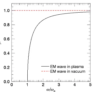
Figure 1.2: The reflectivity of a plasma as a function of its electron number density, normalised to the critical density (equation 1.11).
1.2.6 Critical density
Following the derivation of the dispersion relation for electrostatic and electromagnetic
waves in plasma, it can be shown that electromagnetic waves whose frequencies are less than the plasma frequency cannot propagate through the plasma of the corresponding
density due to screening of the wave’s electric field by the electrons. It is possible to
arrive at a condition for the electron density above which an electromagnetic wave of a given frequency cannot propagate.
Rearranging the plasma dispersion relation above gives:
c2 = ω
2
k2 1−
ωp2 ω2
! .
From this it can be seen that the refractive index of a plasma is given byµ(ω) =
1−ωp2/ω21/2. The reflectivity for a given frequency isR =|(1−µ)/(1 +µ)|2, and is plotted as a function of electron number density in figure 1.2. Three distinct regimes can now be considered.
For waves with ω > ωp, the reflectivity is less than one, and so the wave can
propagate through the plasma. Asω tends to infinity, the refractive index tends toward unity, and the reflectivity to zero, as for vacuum. Ifω < ωp, however,µis imaginary and
frequency greater than the incident wave’s frequency, and will instead be specularly
reflected.
The electron number density corresponding toω =ωpis referred to as the critical
density,nc:
ωp(ne=nc) =ω,
∴nc=
me0ω2
q2
e
. (1.11)
A wave interacting with plasma at the critical density will be reflected (µ= 0, R= 1), and may drive resonant behaviour, an example of which is discussed in section
1.4.2.
1.3
High power lasers
1.3.1 ‘Long-pulse’ lasers
High power lasers are generally divided into two broad categories based on the duration of the laser pulse produced. ‘Long-pulse’ lasers typically have pulse lengths on the order
of a few nanoseconds. Many of the world’s current and planned major high power
laser facilities have multiple long-pulse laser beam lines: NIF (LLNL, 192), UFL-2M (RFNC-VNIIEF, 192 planned), LMJ (CEA, 176), OMEGA (LLE, 60), SG-III (CAEP, 48
planned), Gekko XII (ILE, 12), Orion (AWE, 10), Vulcan (RAL, 6).
Discussions of long-pulse laser interactions and their applications are beyond the scope of this work. Suffice it to say that when employed in conjunction with short-pulse
lasers (discussed below), long-pulse lasers are generally used to compress a target to
high densities, or deliberately ablate some of the surface material to create a region of low density plasma in front of the target which will potentially enhance the fraction of
short-pulse laser energy absorbed.
1.3.2 ‘Short-pulse’ lasers
The development of the chirped pulse amplification (CPA) process in the 1980s [34], and later, optical parametric chirped pulse amplification (OPCPA) [35], permitted the generation of much shorter (∼ 1 ps), and thus higher power (∼ 1 PW), laser pulses.
These high power, short-pulse lasers can be focused to intensities of up to about
much shorter than the normal hydrodynamic response time of the material. This rapid
delivery of energy allows matter to be heated to extreme (hundreds ofeV) temperatures, while remaining at a high (solid) density, resulting in conditions which would otherwise
be very difficult to achieve under laboratory conditions.
Short-pulse laser pulses with energies between approximately 100 and 500 J
typically have pulse durations between several hundred femtoseconds and several
picoseconds. Examples of this type of laser can be found at several laser facilities:
OMEGA-EP (LLE), Vulcan (RAL), Orion (AWE), Titan (LLNL), Trident (LANL), PETAL (CEA), GEKKO XII (ILE), SG-II-U (SIOM). Amplified spontaneous emission
(ASE) and parametric fluorescence in the amplification chain are characteristic features
of CPA and OPCPA lasers. These processes often result in the main pulses delivered by such lasers being preceded by a low intensity, nanosecond-scale duration pre-pulse [36],
which will interact with the target in a similar way to a separate long-pulse laser. Several
techniques have been developed to mitigate the pre-pulse on short-pulse lasers. One of which is to employ a non-linear frequency conversion crystal to convert the laser light
from the first to the second harmonic [37]: since the conversion process has a minimum
intensity threshold, the low intensity pre-pulse passes through the crystal without being converted, and is then spectrally filtered from the converted second harmonic light
[38, 39].
Short-pulse lasers which deliver pulses carrying tens of joules of energy tend to
have pulse durations on the order of tens of femtoseconds. In this way lasers such as
Callisto (LLNL), PEARL (IAP RAS) and Astra Gemini (RAL) are able to achieve the same output power as higher energy short-pulse lasers. Due to the lower energy levels
passing through the laser amplification chain, these lasers have a minimal pre-pulse, and are able to achieve a much higher shot rate (∼10 shots per second cf. ∼5 shots per
day).
By employing a combination of short-pulse and long-pulse beam lines, it is
possible to study the properties of matter compressed to intense pressures (by the long-pulse) and heated to extreme temperatures (by the short-long-pulse). In this way high power
laser facilities facilitate investigations into a range of topics including, but not limited to:
inertial fusion studies [11, 12, 40, 41], radiographic methods such as proton [15–17] and x-ray radiography [18–25], and material properties in astrophysical conditions [27, 28].
1.4
Short-pulse laser absorption
and the laser intensity, pulse length and angle of incidence. The abundance of
absorption mechanisms, with no clear partitions between the regimes in which each occurs, necessitates a detailed numerical approach to modelling short-pulse laser-plasma
interactions in order to capture as much of the pertinent physics as possible. Some of
the main absorption processes are summarised below. For each process the conditions under which it becomes a major means of transferring energy out of the laser pulse are
given.
1.4.1 Inverse bremsstrahlung
An electron, in plasma, oscillating in the electric field of a laser, may collide with a nearby ion, resulting in a transfer of energy. This process is often contrasted
with bremsstrahlung, in which the electron-ion interaction results in the emission of
radiation. Consequently this laser absorption process is commonly referred to as inverse bremsstrahlung. By balancing the rate of change of the electron distribution function
with the collisional heating rate it can be shown that inverse bremsstrahlung acts to drive the electron distribution towards a supergaussian of the formfe∼exp −v5
[42].
Since the presence of an electromagnetic wave is required, inverse bremsstrahlung
can only take place in underdense plasma (electron density is such that the electron plasma frequency is less than the laser frequency). The oscillatory velocity of an
electron is proportional to the electric field amplitude, and since the electron-ion
collision frequency scales inversely with the cube of velocity this process is usually only important for low intensity (. 1016Wcm−2) laser-plasma interactions occurring over
time-scales which are long compared to the electron-ion collision time. This results in
inverse bremsstrahlung being the dominant absorption mechanism for many long-pulse (nanosecond-scale) interactions, such as inertial confinement fusion (ICF).
1.4.2 Resonance absorption
A p-polarised2 electromagnetic wave obliquely incident on a plasma with a density
gradient can propagate up to a density of ne = nccos2θ due to refraction, where
θ is the angle of incidence of the laser measure relative to the target normal, and a
linear density ramp has been assumed. Beyond this density the electric field decays
evanescently, but is still non-zero at the critical surface. At this point the plasma frequency, by definition, matches the frequency of the incident laser, and thus a plasma
wave is resonantly driven [43, 44]. The resonance acts to drive the plasma wave to
2
very large amplitudes until it can no longer be supported and wave breaking occurs,
resulting in the ejection of energetic (fast) electrons from the resonance region. The process of resonance absorption requires moderate (1014–1017Wcm−2) laser intensities
in order for the evanescent field to be strong enough to drive the electrons at the critical
surface, but avoid deformation of the plasma density profile due to the ponderomotive force (discussed later). This process also requires a long scale-length density ramp in
order for the laser to be turned around via refraction.
1.4.3 Vacuum heating
If the scale-length of the plasma density ramp is very short compared to the laser wavelength, vacuum heating occurs [45]. Electrons in the overdense region (densities
such that the electron plasma frequency is greater than the laser frequency) are directly
exposed to the laser’s electric field. Electrons near the surface of the plasma can be pulled, by the electric field of the laser, out of the plasma, beyond the Debye sheath.
As the field reverses polarity the electrons are accelerated back into the plasma. By the time the field reverses again these electrons will have travelled beyond the skin depth
(ls=c/ωp) of the target, and thus are no longer influenced by the laser fields.
1.4.4 Ponderomotive acceleration
The finite size and duration of the laser pulse tends to result in a net force on the electrons, driving them away from regions of high laser intensity. An electron initially at
rest in the middle of a Gaussian laser pulse will move under the influence of the laser’s
electric field. When the field reverses, however, the electron will have moved to a region of lower intensity (and thus field amplitude), and so experiences a weaker restoring
force. Over time this leads to a net drift away from the peak electric field amplitude.
An expression for the laser cycle-averaged ponderomotive force can be derived [46]:
Fp=−
q2
4mω2∇E 2 0,
whereω is the frequency, and E0 the electric field amplitude, of the laser. This effect,
parallel and perpendicular to the laser pulse, can lead to channelling (in underdense
plasma) or hole boring (in overdense plasma). Note that the ponderomotive force is independent of the sign of the charge, and so will also act to expel ions from regions of
high laser intensity. Due to their much higher inertia, however, ion acceleration takes
1.4.5 J ×B force
At high laser intensities (I &1018Wcm−2) the force due to the magnetic field of the laser acting on electrons oscillating in the electric field is non-negligible compared to
the electric field force. The combination of oscillation in the electric field of the laser
perpendicular to an oscillating magnetic field results in a force parallel to the laser axis which varies in time as cos 2ωt. For a lone electron this results in a lemniscate orbit
rather than simple oscillation. If the laser is incident upon an overdense plasma, however,
a similar effect to vacuum heating occurs, except with a longitudinal driving force, due to the magnetic field, at twice the laser frequency [47]. Therefore this acceleration
is characterised by the production of energetic electron bunches, at the second laser
harmonic, directed predominantly along the laser axis.
1.4.6 Other important processes
In addition to the absorption processes above, there are a number of other effects which
manifest themselves during laser interactions. Two examples of such phenomena are given below.
Self-induced transparency
If the electrons in a plasma oscillate at relativistic velocities in the electric field of a laser,
the local plasma frequency decreases. This relativistic behaviour allows a high intensity
laser pulse to propagate beyond the classical critical density surface, and instead be reflected at relativistic critical density,γnc [48].
Relativistic self-focusing
As discussed earlier, the finite size of a laser pulse results in electrons being driven away
from the peak intensity regions by the ponderomotive force. This leads to a depletion of electrons in the centre of the pulse, and an excess in the wings. Since the dispersion
relation for an electromagnetic wave in plasma isω2 = ωp2+c2k2, the phase velocity of the laser is lower in the low density channel carved by the ponderomotive force. The portions of the beam which span the density gradient surrounding the channel
will undergo refraction, resulting in focussing of the beam to higher intensities in the
1.5
Energy transport
1.5.1 Return current generation
The motion of the fast electrons produced by direct laser interaction generates an electrostatic field (via Amp`ere’s law, ∂E/∂t = c2∇ ×B −J/
0). This field acts
upon the background electrons present in the bulk of the target, causing them to drift
toward the laser interaction region (via the Lorentz force,F =q(E+v×B)) in order to restore quasi-neutrality. This motion also helps to replenish the electron population
available for acceleration by the laser.
The return current density due to an imposed fast electron current is related to the electric field via Ohm’s law: Jb = E/η, where η = me/q2enbτc is the
plasma resistivity, and τc is the characteristic background electron-ion collision time.
Substituting this into Amp`ere’s law, and assuming magnetic field effects can be neglected (i.e. that the problem is one-dimensional), yields the following relation between the
background and fast electron currents:
Jf +Jb =−0η
∂Jb
∂t ,
where, for simplicity, a constant resistivity has been assumed. A return current of the form Jb =Jf e−t/τ−1
can be substituted into the
above, and results in an expression for the response time of the plasma to changes in
the fast electron current [51]: τ =0η.
For most conditions of interest this response time is much shorter than the plasma
period, ωp−1, and so the return current is often assumed to respond instantaneously to changes in the fast electron current.
1.5.2 Ohmic heating
Since the background electron density is usually much greater than the density of the
fast electrons, their drift velocity does not need to be very large in order for the counter-propagating currents to balance. Since their velocity is low, the background electrons
are highly collisional compared to the fast electrons, and so act to heat the plasma. In
this way laser energy can be coupled to the target beyond the laser interaction region, and any associated thermal conduction front, via the return current drawn by the fast
electrons.
The rate of change of the background electron energy density, Wb, due to the
current, is given by [52]:
∂Wb
∂t =E·Jb.
By combining this with the material’s specific heat (CV = (∂Wb/∂T)V /nb), it is
possible to calculate the Ohmic heating rate:
∂Tb
∂t =
1
nbCV
∂Wb
∂t =
E·Jb
nbCV
. (1.12)
1.5.3 Filamentation
The transport and deposition of energy inside the target is further complicated by the
fast electrons’ self-generated magnetic fields, which have been neglected thus far. In
some cases these fields can act to collimate the fast electron beam [53]. More often, though, noise in the fast electron current density, background resistivity and/or
small-scale magnetic fields inside the target lead to the fast electron population breaking up
into filaments [54, 55]. The magnetic fields associated with these localised regions of higher current act to deflect fast electrons towards regions of higher current density,
enhancing the filamentation. More recently, studies of the radiation and particles emitted from the rear of laser-irradiated targets have allowed for investigations into the effect of
electrical conductivity [56, 57] and lattice structure [58] on fast electron filamention.
1.5.4 X-ray emission
As fast electrons travel through cold, dense material they undergo elastic scattering off of the background ions. This results in the emission of bremsstrahlung (‘braking radiation’),
providing a broadband x-ray source. Line emission results from a fast electron colliding
inelastically with a bound, inner shell electron, liberating or promoting it to a higher energy level. As an electron relaxes to fill the vacancy, a photon is emitted.
The bremsstrahlung emission is dependent upon the laser and plasma parameters
(the former tend to determine the incident fast electron energy, while the latter determine the bremsstrahlung cross-section), and results in a continuous x-ray spectrum typically
ranging from hundreds ofeV to tens ofMeV.
Line emission, however, is characterised by intense, narrowband peaks in intensity at energies up to approximately100 keV. The precise energies depend upon the atomic
structure of the target’s constituent element(s). By examining the width of the lines,
1.6
Summary of short-pulse laser interactions
Several examples of the principal means for short-pulse laser energy to be absorbed by
a plasma have been discussed above. It is worth noting that all of these processes rely
on the motion of the electrons in the laser’s electromagnetic fields. Due to their much larger mass (and thus, inertia), the ions in the plasma respond very slowly compared to
the laser pulse duration. Many of the ion dynamics occur as a result of fast electrons
setting up large electrostatic fields via charge separation either at the front of the target, as they travel away from the laser interaction region, or at the rear surface, as they exit
the target. Furthermore, many of the above processes are collisionless processes; the
fast electrons they produce travel a significant distance away from the laser interaction region, and heating occurs mainly via Ohmic heating due to a return current. This is
in contrast to long-pulse laser interactions which tend to be dominated by ion motion,
with the electrons primarily acting as a means of transferring the laser energy to the plasma via collisional processes such as inverse bremsstrahlung, and heating occurring
predominantly via thermal conduction [60].
It should be clear from the previous sections that the means by which short-pulse laser energy is delivered to a target, distributed amongst the constituent particles
and transported into the target are complex and interdependent [61, 62]. For this
reason analytic models are generally unable to encompass the full range of phenomena resulting from short-pulse laser interactions. A strong predictive computational
modelling capability is essential in order to support, develop or challenge these models.
Furthermore, such a capability enables the design of laser experiments to be optimised in order to make the best possible use of the capabilities of high power laser facilities
such as OMEGA-EP, Orion and Vulcan-PW.
Computational models already exist which can accurately model the absorption
of a short-pulse laser and production of energetic charged particles. Other methods
also exist for modelling the transport of a pre-defined charged particle distribution and the related energy deposition in the bulk of a laser target. By coupling these
approaches full-scale simulations of short-pulse laser experiments can be performed
[30, 31]. Only recently, however, have algorithms been developed which make self-consistently modelling both the laser absorption and energy transport within a single
simulation tractable [32]. These techniques (integrated modelling and novel high density
1.7
Short-pulse laser applications
1.7.1 Material heating
As discussed in sections 1.4 and 1.5, high power short-pulse lasers provide a means of delivering energy to material samples on time-scales shorter than the typical
hydrodynamic response time. The associated rapid heating permits investigation into the properties of matter at high density (∼ solid) and high temperature (hundreds of
eV) [5–9]. Using a separate long-pulse beam to compress the target prior to the
short-pulse laser interaction further extends the upper limit on the range of densities at which
high temperature material properties can be investigated.
1.7.2 X-ray sources
Some laser experiments make use of a bright x-ray source to backlight the experiment.
This is achieved by fielding a separate target (typically a thin foil [21, 24] or wire
[22, 23, 63]), which is hit by a short-pulse laser to produce x-rays via line emission (see section 1.5.4). The choice of backlighter material is an important consideration, as it
should emit x-rays of sufficient energy that not all of the photons are stopped/scattered
inside the target. Furthermore, the emission energy must not coincide with a peak in the material’s absorption spectrum. For some experiments the x-ray energies produced
by line emission are not sufficient, due to the desire to image very high density materials. In these cases high energy (∼MeV) bremsstrahlung x-rays can be used for radiography
[18–20, 25].
1.7.3 Electron acceleration
As a laser pulse propagates through underdense (ne < nc) plasma, it pondermotively
drives electrons laterally out of the laser pulse, creating a wake of lateral plasma
oscillations. As the laser pulse continues to propagate, these electrons are accelerated
back toward the central axis of the laser pulse, and thus a longitudinal modulation in the electric field is created, trailing the laser pulse. This wakefield is maximised if the laser’s
pulse length is tuned so as to match half the plasma period (τL ≈ π/ωp). Electrons
are then accelerated to very high energies (hundreds ofMeV) over a few centimetres by ‘surfing’ the laser wakefield [64]. By exploiting this, and other similar phenomena, it is
thought that it may be possible to use short-pulse lasers to accelerate electrons up to,
1.7.4 Proton acceleration
When the fast electrons produced by a short-pulse laser-plasma interaction reach the rear surface of the target, those with sufficient energy will leave the target. In doing so
an electric field is set up perpendicular to the rear surface of the target. Protons initially
present on the rear surface of the target (from water or oil surface contaminants) are accelerated to tens ofMeV, over tens of microns, by this field [68–73]. This process is
referred to as target normal sheath acceleration (TNSA).
Alternative methods for accelerating protons using high intensity short-pulse lasers have been proposed, such as the break-out afterburner (BOA) [74] and radiation
pressure acceleration (RPA) [75, 76] approaches. These schemes aim to make use of the
ponderomotive force of the laser pulse to accelerate thin (<1µm) foil targets, either via the electrons (BOA) or by directly accelerating the ions (RPA).
Possible applications of laser-accelerated protons include cancer therapy [13, 14], radiography [15–17], material heating [28, 77–79], and material activation for nuclear
physics [26].
1.7.5 Fast ignition
The pursuit of inertial confinement fusion (ICF) [40, 41] has led to the development of novel schemes to relax the stringent symmetry conditions imposed by the standard
central hot spot ignition technique. The fast ignition approach [11] uses a high intensity,
short-pulse laser to accelerate particles, usually electrons, up to energies such that they travel beyond the interaction region and deliver their energy to the core of a compressed
fusion capsule, as shown in figure 1.3a. Ignition of the fuel capsule places constraints
on the divergence, energy and duration of the fast electron beam.
Ablation of the capsule surface tends to result in the critical surface being located
several hundred microns from the compressed core. Therefore a means is required by
which the short-pulse laser can be allowed to interact as close to the anticipated hot spot as possible. One technique is to use a separate short-pulse beam, co-linear with the
main pulse, and the ponderomotive hole-boring process [1] to carve a low density channel
through the ablated coronal region, down which the main pulse can then propagate with minimal energy loss. An alternative concept, which has received a significant amount of
attention, is to ensure a clear path for the ignition beam by having a high density cone (usually gold) inserted into the fuel capsule [12] as shown in figure 1.3b. The purpose
of the cone being to prevent ablated material from the capsule from entering the path
(a) The fast ignitor concept as originally proposed by Tabak et al. [11].
[image:39.595.127.511.120.274.2](b) The cone-guided fast ignition approach proposed by Kodama et al. [12].
Figure 1.3: Diagrammatic representation of the fast ignition concept as originally envisaged (a) and with a gold cone insert (b). Reproduced with permission from Sircombe [80].
1.8
Overview of plasma modelling
Plasma physics modelling codes are widely employed in topics such as astrophysics, solar
physics, magnetic and inertial confinement fusion, and laser-plasma interactions. Detailed modelling of short-pulse (picosecond-scale) laser experiments requires
capturing phenomena which occur on spatial and temporal scales which span several
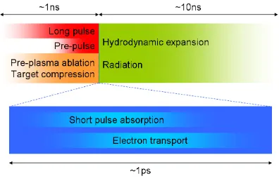
orders of magnitude (as illustrated by figure 1.4). The main pulse is typically preceded by an ASE (amplified spontaneous emission) pedestal, commonly referred to as a pre-pulse,
of approximately nanosecond duration. Some experiments also make use of a separate
long-pulse (nanosecond-scale) beam. These act to ablate the surface material creating a region of high temperature, low density plasma in front of the target (pre-plasma).
Immediately behind the ablation front, the high thermal pressure results in a shock
being driven into the target, compressing the material. Following the laser interaction the target undergoes hydrodynamic expansion and disassembly, while radiating heat
(typically as x-rays), over several nanoseconds. In contrast, the fast electron transport
and associated target heating typically occurs on time-scales comparable to the main short-pulse laser duration [81]: up to a few picoseconds, necessitating a separate, more
detailed treatment than the other phases.
The mechanisms by which the short-pulse laser delivers its energy to the target,
how this energy is distributed amongst the particles, and how it is transported deeper
Figure 1.4: Visual representation of the disparate time-scales involved in short-pulse laser interactions.
temporal scales smaller than the laser period and the period of Langmuir waves in the
plasma. Furthermore, it is essential that one accurately resolves the non-thermal nature of the electron distribution function. Key to short-pulse modelling is the kinetic nature
of the plasma—but in treating this problem with such high fidelity it is not feasible to consider the much longer time-scale hydrodynamic phases.
Thus many disparate approaches to modelling laser-plasma physics phenomena
are employed. These fall into two main categories: fluid and kinetic models.
1.8.1 Fluid models
Fluid models, in general, assume that the plasma at any point in space can be
characterised by macroscopic quantities derived from moments of the particle
distri-bution functions (namely, density, centre-of-mass velocity and temperature). Since each moment is a function of the next highest order moment, fluid models often invoke an
equation of state, which relates the internal energy to the density and pressure, in order to
obtain a closed set of equations. When attempting to model phenomena on large spatial and temporal scales this assumption is generally valid, and the magneto-hydrodynamic
influence of electromagnetic fields. This makes hydrocodes powerful tools for simulating
bulk behaviour during laser-plasma interactions. However, the fluid model is no longer valid when attempting to model phenomena which involve significant deviation from a
Maxwellian particle distribution and/or motion which is dominated by non-linear
wave-particle interactions, such as stimulated Raman scattering [83, 84], Landau damping [85], resonance absorption [43, 44], Brunel vacuum heating [45] and ponderomotive
acceleration [46].
1.8.2 Kinetic models
The statistical treatment employed in kinetic models retains the individual particle properties, rather than integrating over the local distribution. The particles are
considered to be evolving in time within a six-dimensional phase-space—three physical
dimensions (x,y,z) and three momentum dimensions (px,py,pz). The evolution of the
distribution function, f, of a particle species, in the presence of electric and magnetic
fields, is governed by the plasma kinetic equation (see section 1.2.1):
∂f
∂t +v· ∇f+ q
m(E+v×B)· ∇vf =
∂f ∂t
coll
.
The additional physics embodied by kinetic codes carries with it an increase
in the complexity of the codes. Thus the main limitation of kinetic codes is the high computational cost associated with modelling individual particle behaviour. This severely
reduces the spatial and temporal scales that can be modelled efficiently compared with
fluid methods.
1.8.3 Hybrid models
Occasionally both fluid and kinetic models are employed within the same code. These
hybrid codes generally model an energetic particle species using a kinetic approach,
and treat the background material (which is often at a lower temperature and higher number density) as a (multi-component) fluid. This approach has been used successfully
to model energy transport in laser-plasma interactions [54, 86–88], but is unable to
accurately model systems in which the kinetic and fluid populations cannot be treated as separate, for example the absorption of laser energy and production of fast electrons
1.8.4 Summary of plasma models
The choice of code to use when simulating plasma physics is dependent on the complexity of the system and the spatial and temporal scales of interest. Fluid models are useful in
modelling the relatively slow, large-scale bulk motion of the plasma. In contrast, when
Chapter 2
Overview of the
EPOCH
PIC code
2.1
Particle-in-cell codes
The most rigorous approach to kinetic modelling is that employed by Vlasov codes,
such as IMPACT [89], KALOS [90], VALIS [91], FIDO [92, 93] and OSHUN [94]. These simulate the plasma by solving the plasma kinetic equation directly, using a variety of
approaches. For example, in Eulerian codes such as VALIS and FIDO, the particle distribution functions are evolved on an N-dimensional phase-space grid, where N is the number of spatial and momentum dimensions being simulated. Thus a 2D3P
Eulerian Vlasov code requires a five-dimensional grid (two space and three momentum
dimensions—x, y, px, py, pz; or x, y,|p|, θ, φ in the case of FIDO). The requirements
of high dimensionality and high resolution in each dimension mean that such codes
can be very computationally intensive. IMPACT also employs an Eulerian phase-space grid, but employs the diffusion approximation [89] to reduce the number of momentum dimensions required. Although this approach is well suited to simulating fast electron
transport through dense plasma, it is not conducive to modelling oscillatory phenomena
such as laser-plasma interactions. Codes such asKALOS andOSHUN, however, represent the distribution function in momentum space using an series expansion in spherical
harmonics. This approach is also well suited to modelling fast electron transport. The
use of spherical harmonics also reduces the computational expense associated with the distribution function representation in momentum space, but can suffer from difficulties
with ensuring that mass is conserved, and that the distribution function is positive
everywhere [90].
For most ‘everyday’ purposes a more general ‘workhorse’ code is required which
can perform a broad range of kinetic simulations to an adequate level of precision and
![Figure 1.3:Diagrammatic representation of the fast ignition concept as originallyenvisaged (a) and with a gold cone insert (b).Reproduced with permission fromSircombe [80].](https://thumb-us.123doks.com/thumbv2/123dok_us/9529638.458077/39.595.127.511.120.274/figure-diagrammatic-representation-ignition-originallyenvisaged-reproduced-permission-fromsircombe.webp)


![Figure 2.6: The dispersion relations for an electromagnetic wave propagating on adiscrete, 1D mesh, with varying time-step durations [95].](https://thumb-us.123doks.com/thumbv2/123dok_us/9529638.458077/58.595.174.444.131.392/figure-dispersion-relations-electromagnetic-propagating-adiscrete-varying-durations.webp)

