warwick.ac.uk/lib-publications
Original citation:
Georgakopoulos, Agelos. (2016) The boundary of a square tiling of a graph coincides with
the Poisson boundary. Inventiones Mathematicae, 203 (3). pp. 773-821.
Permanent WRAP URL:
http://wrap.warwick.ac.uk/79554
Copyright and reuse:
The Warwick Research Archive Portal (WRAP) makes this work by researchers of the
University of Warwick available open access under the following conditions. Copyright ©
and all moral rights to the version of the paper presented here belong to the individual
author(s) and/or other copyright owners. To the extent reasonable and practicable the
material made available in WRAP has been checked for eligibility before being made
available.
Copies of full items can be used for personal research or study, educational, or not-for profit
purposes without prior permission or charge. Provided that the authors, title and full
bibliographic details are credited, a hyperlink and/or URL is given for the original metadata
page and the content is not changed in any way.
Publisher’s statement:
“The final publication is available at Springer via
http://dx.doi.org/10.1007/s00222-015-0601-0
."
A note on versions:
The version presented here may differ from the published version or, version of record, if
you wish to cite this item you are advised to consult the publisher’s version. Please see the
‘permanent WRAP url’ above for details on accessing the published version and note that
access may require a subscription.
arXiv:1301.1506v2 [math.PR] 23 Jan 2014
The Boundary of a Square Tiling of a Graph
coincides with the Poisson Boundary
Agelos Georgakopoulos
∗Mathematics Institute
University of Warwick
CV4 7AL, UK
January 24, 2014
Abstract
Answering a question of Benjamini & Schramm [8], we show that the Poisson boundary of any planar, uniquely absorbing (e.g. one-ended and transient) graph with bounded degrees can be realised geometrically as a circle, namely as the boundary of a tiling of a cylinder by squares. This implies a conjecture of Northshield [34] of similar flavour. For our proof we introduce a general criterion for identifying the Poisson boundary of a stochastic process that might have further applications.
1
Introduction
1.1
Overview
In this paper we prove the following fact, conjectured by Benjamini & Schramm [8, Question 7.4.]
Theorem 1.1. IfGis a plane, uniquely absorbing1graph with bounded degrees,
then the boundary of its square tiling is a realisation of its Poisson boundary.
The main implication of this is that every such graphGcan be embedded inside the unit disc D of the real plane in such a way that random walk on
Gconverges to ∂Dalmost surely, its exit distribution coincides with Lebesgue measure on∂D, and there is a one-to-one correspondence between the bounded harmonic functions on G and L∞(∂D) (the innovation of Theorem 1.1 is the last sentence).
Knowing that a graphGis not uniquely absorbing provides a lot of informa-tion about its Poisson boundary; in particular,Gis not Liouville. Thus it is not a significant restriction in our context to assume thatGis uniquely absorbing. We use Theorem 1.1 to prove a conjecture of Northshield [34] of similar flavour (Conjecture 8.1), thus obtaining a further geometric realisation of the Poisson boundary of the graphs in question.
In the case whereGis hyperbolic, we can say a bit more:
∗Partly supported by FWF Grant P-24028-N18.
Corollary 1.2. Let G be an infinite, Gromov-hyperbolic, non-amenable, 1-ended, plane graph with bounded degrees and no infinite faces. Then the fol-lowing five boundaries of G(and the corresponding compactifications ofG) are canonically homeomorphic to each other: the hyperbolic boundary, the Mar-tin boundary, the boundary of the square tiling, the Northshield circle, and the boundary ∂∼=(G).
We present examples showing that all these conditions are necessary to make the statement true and none of them is implied by the others, except that it is not clear whether both the bounded degree and the non-amenability conditions are necessary; see Problems 8.3 and 8.4. The least obvious case is to show that hyperbolicity is not implied by the other properties, contrary to another conjecture of Northshield [34]; we disprove that conjecture by a counterexample in Section 8.2.
The equivalence of the Martin boundary to the hyperbolic boundary in Corollary 1.2 follows from a result of Ancona [1, 2] that can be thought of as a discrete version of the theorem of Anderson & Schoen [3] that for any complete, simply connected Riemannian manifold with bounded and negative sectional curvatures, the Martin boundary with respect to the Laplace-Beltrami operator coincides with the geometric boundary. This motivates
Conjecture 1.1. Let M be a complete, simply connected Riemannian surface
with Gaussian curvatures bounded between two negative constants. Letf :M →
Dbe a conformal map fromM to the open unit disc inC. Then for every 1-way infinite geodesic γ inM, the image f(γ) converges to a point in the boundary S1 of D, and this convergence determines a homeomorphism from the sphere at infinity of M toS1. (In particular, images of equivalent geodesics converge to the same point of S1.)
For the proof of Theorem 1.1 the following criterion for identifying the Pois-son boundary of a general Markov chain is introduced, that might have further applications. A functionh:V →[0,1] issharp, if its values along the trajectory of the Markov chain converge to 0 or 1 almost surely.
Theorem 1.3. Let M be an irreducible Markov chain and N an M-boundary.
Then N is a realisation of the Poisson boundary ofGif and only if it is faithful to every sharp harmonic function.
Loosely speaking, Theorem 1.3 states that in order to check that a can-didate space is a realisation of the Poisson boundary, it suffices to consider its behaviour with respect to the sharp harmonic functions rather than all bounded harmonic functions. This fact, and its proof, can be generalised to many con-tinuous stochastic processes. We will have a closer look at Theorem 1.3 and its implications in Section 1.4, after some background information.
1.2
Square tilings —a discrete analogue of conformal
uni-formization
eofGcorresponds to a squareRe in the tiling and every vertexxcorresponds
to an interval tangent with all squares corresponding to the edges of x. The construction was made using an electrical current on the graph, and the square Reis given side length equal to the current going throughe, while the position
of Re is determined by the voltages of the vertices (see Section 5 for details).
This construction has become a classic, with a lot of applications ranging from recreational mathematics to statistical mechanics; see e.g. [12, 15, 30, 31].
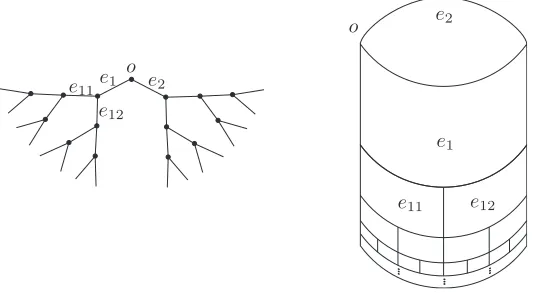
Benjamini and Schramm [8] showed that the construction of [10] can be applied to an infinite planar graphG in the uniquely absorbing case; the elec-trical current now emanates from a single vertexoand escapes to infinity, and is intimately connected to the behaviour of random walk from o. The square tiling takes place on the cylinderK=R/Z×[0,1], the edges of the graph being mapped to disjoint squares tiling K; see Figure 1 or [8, FIG. 1] for examples. Their motivation was to find discrete analogues of Riemann’s mapping theorem; the following quote is from [8]
“The tiling plays the same role as conformal uniformization does for planar domains. In fact, the proof of its existence illustrates parallels with the continuous theory. In a way, it is a discrete analogue of Riemann’s mapping theorem.”
For more on the relationship between square tilings and Riemann’s mapping theorem see [11]. The paper [7] is similar in nature to [8] and provides a further discrete analogue of Riemann’s mapping theorem. A well known corollary of both [7, 8] is that every planar transient graph admits non-constant harmonic functions of finite energy. This result, in fact a detailed description of the space of such functions, can now be derived combining Theorem 1.1 with the results of [20].
o
o e1
e1
e2
e2
e11
e11
e12
[image:4.595.165.432.455.603.2]e12
Figure 1: The infinite binary tree and its square tiling.
1.3
The Poisson boundary of a stochastic process
The Poisson(-Furstenberg) boundary of a transient stochastic process M is a measure spaceP associated withM such that every bounded harmonic function on the state space ofM can be represented by an integral onP and, conversely, every function inL∞(P) can be integrated into a bounded harmonic function of
M. The standard example [18, 24] is whenM denotes Brownian motion on the open unit disc Din the complex plane; then the classical Poisson integral rep-resentation formula h(z) = R1
0
1−|z|2
|e2πiθ−z|2hˆ(θ)dθ =
R1
0 hˆ(θ)dνz(θ) recovers every continuous harmonic function h from its boundary values ˆhon the circle ∂D. Here,νz is theharmonic measure on∂D, i.e. the exit distribution of Brownian
motion started atz, and can be obtained by multiplying the Lebesgue measure by the Poisson kernel |e21πiθ−|z−|2z|2. Thus, we can identify the Poisson boundary of Brownian motion M on D with ∂D, endowed with the family of measures
νz, z∈D.
In this example, the boundary was geometric and obvious. If M is now an arbitrary transient Markov chain, then there is an abstract construction of a measurable space P, called the Poisson boundary of M, endowed with a family of measuresνzindexed by the state spaceV ofM, such that the formula
h(z) = R
Pˆhdνz provides an isometry between the Banach space H∞(M) of
bounded harmonic functions ofM (endowed with the supremum norm) and the spaceL∞(P).
Triggered by the work of Furstenberg [18, 19], a lot of research has con-centrated on identifying the Poisson boundary of various Markov chains, most prominently locally compact groups endowed with some measure; see [1, 25, 26, 28] just to mention some examples, and [16] for a survey including many ref-erences and some impressive applications. However, I would like to stress that this paper is not about groups (although some of its techniques might be appli-cable to them), but rather about extending the study of the Poisson boundary to embrace general graphs, a currently emerging quest [4, 20].
In general, one would like to identify the Poisson boundary of a given Markov chain with a geometric object as we did for D, which could for example be a compactification of a Cayley graph on which our group acts. This task can however be very hard. Some general criteria have been developed for the case of groups, mostly by Kaimanovich [24, 26], that have helped to identify ‘geometric’ Poisson boundaries for certain classes of groups e.g. hyperbolic groups, but others, like the lamplighter group overZ3 [17], defy such identification despite extensive efforts. A well-known open problem is whether the Liouville property, which can be expressed as triviality of the Poisson boundary, for simple random walk on a Cayley graphG=Cay(Γ, S) is a group invariant, i.e. independent of the choice of the generating set Sof a given group Γ.
1.4
More on our results
There are various definitions of the Poisson boundary for general Markov chains in the literature. In this paper, rather than choosing one of them, or introducing our own, we will follow a more flexible approach, accepting any measure space that fulfils the properties expected from “the” Poisson boundary as “a” Poisson boundary. More precisely, given a transient Markov process M, we let anM -boundary, or a G-boundary if M happens to be random walk on a graph G, be any measurable space N endowed with a family of measures (νz), z ∈ V
(recall our D example) and a measurable, measure preserving, shift-invariant function f from the space of random walk trajectoriesW to N; see Section 3 for details. This definition is rather standard [24]. We say that anM-boundary
N is arealisation of the Poisson boundary of M, if every bounded harmonic function h on the state space V of M can be obtained by integration of a bounded function ˆh∈L∞(N), where this ˆhis unique up to modification on a
null-set, and conversely, for every ˆh∈L∞(N) the functionf :V →Rdefined
byz7→R
Nhˆ(η)dνz(η) is bounded and harmonic.
Recall the definition of a sharp function from Section 1.1. In Section 3 we introduce ‘intersection’ and ‘union’ operations between pairs or families of sharp harmonic functions using probabilistic intuition, and show that the familyS of sharp harmonic functions of a Markov chain is closed under these operations. ThusS carries aσ-algebra structure, except that there is no ground set. Theo-rem 1.3 can be interpreted in the following way: anyM-boundaryN that can be used as the ground set for thisσ-algebra structure, with its measures agreeing with corresponding probabilities defined with respect to sharp harmonic func-tions, is a realisation of the Poisson boundary. A bit more precisely, if N is faithful toS, that is, if for every measurable subset X ofN there iss∈ S such that almost surely random walk ends up inX if and only if the values ofsalong its trajectory converge to 1, thenN is a realisation of the Poisson boundary.
A direct implication of the comparison of the σ-algebra structure of S to that ofN is that any two realisations of the Poisson boundary ofM are cryp-tomorphic, see Corollary 3.5 (this fact will not be surprising to experts).
Given a Markov chain it is often easy to guess a realisation of its Poisson boundary, most often in the form of some topological space naturally associated to the chain, e.g. the boundary of a compactification, but it is much harder to prove that the guess is correct. Our case, the boundary of a square tiling, is such an example. Other examples include the end-compactification of a tree, and the hyperbolic boundary of a hyperbolic group [24]. The following tool, abstracted from the proof of Theorem 1.1 via Theorem 1.3, may be helpful in further such cases. A topological G-boundary of a graph G is a topological space (N,O) endowed with a ‘projection’τ :V → O so that τ(Zn) converges
to a point in N for almost every random walk trajectory Zn, and there is a
Borel-measurable function τ∗ : W → N mapping almost every (Zn) ∈ W to
limnτ(Zn). Note that defining νz byO ∈ O 7→ µz(τ∗−1(O)) turns N into a
G-boundary for f = τ∗. We say that (N, τ) is layered, if there is a sequence (Gn)n∈N of finite subgraphs ofG with SGn = G the boundaries (Bn)n∈N of
which satisfy µn
z(b) = νz◦τ(b) for every b ∈ Bn, where µnz denotes the exit
distribution ofGn for random walk fromz.
G-boundary with projection τ. If for every sharp harmonic function swe have limm,nν(τ(Fm)△τ(Fn)) = 0, where Fi := {b ∈ Bi | s(b) > 1/2}, then N
endowed with the measures(νz)as above is a realisation of the Poisson boundary
of random walk onG.
The following observation, proved in Section 6.1, is one of the main tools in the proof of Theorem 1.1 and might be of independent interest. Here, a graph is considered as a metric space where every edge is a copy of the real unit interval, and so each square of the tiling is foliated into horizontal intervals, one for each inner point of the corresponding edge.
Observation 1.5. LetGbe a plane, uniquely absorbing graph and consider its
square tiling T of the cylinder K. For any circleL⊂K parallel to the base of K, letB be the set of points ofGthe images of which lie in L. Then the widths w(T(b)), b∈B of these images coincide with the exit probabilities of standard brownian motion on Gstarted at the reference vertexoand killed atB.
Our proof of Theorem 1.1 applies to a larger class of graphs where the degrees are not necessarily bounded, see Corollary 7.8. Such graphs have attracted a lot of interest lately, see [23] and references therein.
We prove Theorem 1.3 in Sections 3 and 4 and Theorem 1.1 in Section 7, after constructing the square tiling in Section 5 and proving some general prop-erties, including interesting probabilistic interpretations of its geography like Observation 1.5, in Section 6. We deduce Corollary 1.4 in Section 7.3.
2
Preliminaries
LetG = (V, E) be a graph fixed throughout this section, whereV =V(G) is its set of vertices and E =E(G) its set of edges. A walk on Gis a (possibly finite) sequence (vn)n∈N of elements of V such that vi is always connected to
vi+1 by an edge. More generally, we define a walk on the state spaceV of a Markov chain in a similar manner, where we might or might not demand that the transition probabilitiespvi→vi+1 be positive.
A plane graph is a graphG endowed with a fixed embedding in the plane R2; more formally,Gis a plane graph ifV(G)⊂R2 and each edgee∈E(G) is an arc between its two vertices that does not meet any other vertices or edges. A graph is planar if it admits an embedding in R2. Note that a given planar graph can be isomorphic (in the graph-therotic sense) to various plane graphs that cannot necessarily be mapped onto each other via a homeomorphism of R2.
A plane graphG⊂R2isuniquely absorbing, if for every finite subgraphG0 there is exactly one connected componentDofR2\G0that isabsorbing, that is, random walk onGvisitsG\Donly finitely many times with positive probability (in particular, G is transient). Uniquely absorbing graphs are precisely those admitting a square tiling. Example classes include all transient 1-ended planar graphs, which includes the bounded-degree 1-ended planar Gromov-hyperbolic graphs, all transient trees and, more generally, all transient graphs that can be embedded inR2 without accumulation points of vertices.
Arandom walkonGbegins at some vertex and when at vertexx, traverses one of the edges−xy→incident toxaccording to the probability distribution
px→y :=
c(xy) πx
, (1)
where πx :=Py∈N(x)c(xy) and N(x) denotes the set ofneighbours ofx, that is, the vertices connected toxby an edge. Whenc= 1, which is the case most often considered,πxcoincides with thedegree ofx, and we havesimple random
walk, i.e.y is chosen according to the uniform distribution onN(x).
Formally, there are two standard ways of rigorously formalising random walk as a probability space: the first is as a Markov chain in the obvious way. The second, and the one that we will adhere to in this paper, is by considering random walk on G as a measurable space (W,Π), endowed with a family of measures (µz)z∈V indexed by the vertices of G, where W is the set of 1-way
infinite walks on G, called path space, Π is the σ-algebra on W generated by thecylinder sets, i.e. subsets ofW comprising all walks having a common finite initial subwalk, and µz is the probability measure on (W,Π) corresponding to
fixingzas the starting vertex. Note that oncezis fixed, (1) uniquely determines µz; see [39] for details.
For convenience, we will also assume that every Markov chain M in this paper is formally given in the above form, that is, a choice of a (possibly random) starting pointoand a family of measures (µz)z∈V on path space (W,Π), where
V denotes the state space of M and µz is the law of M conditioning on the
starting point being z. In other words, we formalize M as a random walk on V; in contrast to the random walk on a graph defined above, such random walk need not be reversible, see [32].
It will be convenient in some cases to think of our graphGas a metric space constructed as follows. Start with the discrete setV, and for every edgexy∈E joinxtoyby an isometric copy of a real interval of length 1/c(e) (theresistance ofe). Then, one can consider a brownian motion on this space (as defined e.g. in [5, 33]) that behaves locally like standard brownian motion onR, and it turns out that the sequence of distinct vertices visited by this brownian motion has the same distribution as random walk governed by (1).
A functionh:V →Ron the vertex-set of a graphG, or more generally on the state spaceV of a Markov chain, isharmonic at x∈V if it satisfies
h(x) =P
y∈V px→yh(y), (2)
where againpx→y denotes the transition probability, and it is called harmonic
if it is harmonic at everyx.
A fundamental property of harmonic functions is that their values inside a set are determined by the values at the boundary of that set; to make this more precise, let B be a subset of V, and xa vertex such that random walk from x visits B almost surely; for example, B could be the boundary of a ball of Gcontainingx. Then, lettingbbe the first vertex ofBvisited by random walk fromx, we have
In other words, the boundary values of a harmonic function uniquely determine the function.
We say that random walkhits B atb∈Bif the first element of Bit visit is b.
The following fact, which is a special case of Levy’s zero-one law [27], will come in handy in many occasions
For every µ-measurable event A ⊆ W, random walk Zn satisfies
limnµZn(A) = 1A almost surely. In particular, µZn(A) converges to
0 or 1.
(4)
Here,1A is as usual the characteristic function (fromW to 0,1) ofA. In other words, if we observe at each stepi of our random walk the probability pi that
Awill occur given the current position (the past does not matter because of the Markov property), then almost surelypi will converge to 1 andAwill occur or
pi will converge to 0 andAwill not occur.
For a walkW ∈ Wdefine theshiftt(W) to be the walk obtained fromW by deleting the first step. An eventA⊆ W is called if tail event if t(A) =A (we could be less strict here and write µ(t(A)△A) = 0 instead, where △ denotes symmetric difference).
3
Sharp functions and the Poisson boundary
Let M =Z1, Z2, . . . be an irreducible Markov chain with state space V fixed throughout this section. Call a harmonic function h : V → R+ sharp, if the range of his [0,1] and limnh(Zn) equals 0 or 1 almost surely (the limit exists
almost surely by the bounded martingale convergence theorem). Note that whether h is sharp or not does not depend on the (possibly random) starting pointo, for ifris any other element ofV then, by irreducibility, the probability to visit r from o is positive. Let S =S(V) denote the set of sharp harmonic functions onV.
Lemma 3.1. If h(z) :V →[0,1]equals the probability that random walk from
z will satisfy a tail event Afor every z, thenhis a sharp harmonic function. Proof. The fact thathis harmonic follows immediately from the fact thatAis a tail event and the Markov property. Sharpness follows from (4).
Lets∈ S and fixz ∈V. Define the real valued random variable Xn to be
s(Zn) where Zn denotes random walk from z. Define the random variable X
by lettingX = lims(Zn) if this limit exists (which it does almost surely by the
bounded martingale convergence theorem), andX = 0 otherwise. Since almost sure convergence implies weak convergence [29], we immediately obtain
The sequenceXn converges weakly toX. (5)
Alternatively, let (Bn)n∈Nbe a sequence of subsets ofV such that our Markov
chain visits everyBn almost surely, and letXn =s(Ztn), wheretn is the first
time t such thatZt∈ B
n (if no sucht exists, which happens with probability
0, we can let Xn = 0 to make sureXn is always defined). Then lims(Xn) still
Assis harmonic, we have
s(z) =E[Xn]. (6)
Given z∈V, let 1s be the event, in the path spaceW
z, that for random walk
Znfromzwe have lims(Zn) = 1. Note that this event isµ
z-measurable. Define
the event 0ssimilarly.
Corollary 3.2. Ifsis a sharp harmonic function, thens(z) =µz(1s)for every
vertexz.
Proof. Since theXn are uniformly bounded, their weak convergence (5) implies
convergence in L1, that is, lim
nE[Xn] =E[X], whereX is defined as in (5).
Since s is sharp, E[X] equals the probability to have limns(Zn) = 1 by the
definition ofX. Combined with (6) and the definition of ‘sharp’ this completes our proof.
Corollary 3.3. Ifsis a sharp harmonic function that is not identically 0, then
for every ǫ >0there is z∈V withs(z)>1−ǫ.
Proof. Sinces6= 0, there isowiths(o)>0. By Corollary 3.2 the probability to have limns(Zn) = 1 for random walkZn fromo is positive, in particular there
are verticesz withs(z) arbitrarily close to 1.
Given a sequence (sn)n∈Nof sharp harmonic functions, we define theirunion S
si by z 7→ µz(S1si) and their intersection Tsi by z 7→ µz(T1si). The
complement sc
1 ofs1 is the function 1−s1; note that, by Corollary 3.2,sc1(x) =
µx(0s1).
Lemma 3.4. Let (si) be a sequence of sharp harmonic functions. Then the
functions (i) S
si,
(ii) sc
1, (iii) Ts
i,
are also harmonic and sharp.
Proof. Since all these functions are probabilities of tail events of random walk, they are harmonic and sharp by Lemma 3.1.
This means that the family of sharp harmonic functions satisfies the axioms of aσ-algebra, except that it is formally not a family of subsets of a given set. One way to intuitively interpret Theorem 1.3 is to say that if a measure space
N has the ‘same’σ-algebra structure as the family of sharp harmonic functions ofG, and some obvious requirements are fulfilled, thenN can be identified with the Poisson boundary ofG. Let us make this idea more precise.
A M-boundary, or a G-boundary if M happens to be random walk on a graph G, is a measurable space (N,Σ) endowed with a family of probability measures {νz, z ∈ V} and a measurable, measure preserving, shift-invariant
function f : W → N, where W :=S
z∈VWz is the set of 1-way infinite walks
in G. Here, we say that f is measure preserving if νz(X) = µz(f−1(X)) for
is obtained from W by skipping the first step, then f(W) = f(W′); in other words,f can be thought of as a function from the set of equivalence classes with respect to the shift (called ‘ergodic components’ in [24]) to N.
The fact thatf is shift-invariant and measure preserving implies
νz=Py∼zpzyνy. (7)
Indeed, sincef is shift-invariant, random walk fromz ‘finishes’ inX ∈Σ if and only if its subwalk after the first step finishes inX, and so we haveµz(f−1(X)) = P
y∼zpzyµy(f−1(X)). Since we are demanding that f is measure preserving,
our assertion follows.
This means in particular that the measuresνzare pairwise equivalent when
G is connected: if νz(X) > 0 for some set X ∈ Σ, then νy(X) > 0 for any
neighboury ofz.
Letsbe a sharp harmonic function. We say thatN isfaithful tos, if there is X ∈ Σ such that µz(1s△f−1(X)) = 0 for every z ∈ V, where △ denotes
symmetric difference. Note that such a setX is unique up to modification by a null-set ofν.
For every measurable subsetX of N, the function s=sX defined byz 7→
νz(X) is harmonic and sharp by Lemma 3.1. We claim that
µ(1s△f−1(X)) = 0 (8)
To see this, set Φ := f−1(X)△1s, and recall that both f−1(X) and 1s are µ
-measurable events in path space, hence so is Φ. Now note thatµz(f−1(X)△1s) =
µz(1s∩f−1(Xc)) +µz(0s∩f−1(X)),
where we used the fact that µz(1s∪0s) = 1 assis sharp. It is easy to see that
both these summands equal 0 using the definition ofs, the Markov property of random walk, and the fact thatf is measure preserving.
Note that ifN is faithful to every sharp harmonic function, then combined with (8) this means that, up to perturbations by null-sets, the correspondence between measurable subsets ofN and sharp harmonic functions is one-to-one. Combined with Theorem 1.3, this observation yields
Corollary 3.5. If (N,Σ) is a realisation of the Poisson boundary of a graph
G, then there is a bijectionσfrom the set of equivalence classes ofΣ(where two elements are equivalent if they differ by a null-set) to the set of sharp harmonic functions of Gsuch that νz(X) =µz(1zσ([X])) for everyX ∈Σ andz ∈V(G).
Thus any two realisations of the Poisson boundary ofGare cryptomorphic.
4
Proof of the Poisson boundary criterion
We start by proving the easier direction of Theorem 1.3, namely that if N is a realisation of the Poisson boundary then it is faithful to every sharp harmonic function s. For this, givens let ˆs∈L∞(N) be such thats(z) =R
Nsˆ(η)dνz(η)
for everyz.
We claim that ˆs equals 0 or 1 almost everywhere on N. Indeed, sincef is measure preserving, it suffices to prove that µ(f−1(X)∪f−1(Y)) = 1, where
X :={η | ˆs(η) = 1} and Y := {η | sˆ(η) = 0}. For ǫ ∈ (0,1), let Xǫ :={η |
ˆ
By Lemma 3.1 sǫ is harmonic and sharp. Now note that ifsǫ(Wn) converges
to 1 for some walk Wn, then s(Wn) does not converge to 0 or 1. But as s is sharp, this occurs with probability 0 for our random walk. Since sǫ is sharp,
this implies thatsǫ(Wn) converges to 0 for almost every random walkWn. But
now Levy’s zero-one law (4) implies that µz(f−1(Xǫ)) = 0 for every z. Since
this holds for everyǫ, our claim follows.
As ˆs equals 0 or 1 almost everywhere on N, we have s(z) =νz(X) by the
choice of ˆs and X. Thus (8) yields µz(1s△f−1(X)) = 0, which means thatN
is faithful tosas desired.
4.1
Splitting
N
according to the values of
h
In this section collect some lemmas that will be useful in the proof of the other direction of Theorem 1.3. The reader may choose to skip to Section 4.2 at this point and come back later.
We denote the set of bounded harmonic functions ofGbyBH(G).
Lemma 4.1. Let Gbe a transient network. For every h∈BH(G) and every
a < b∈R, the functionh[a,b)defined byz7→µz(limnh(Zn)∈[a, b))is harmonic and sharp.
Proof. To begin with, it is easy to check that the event{limnh(Zn)∈[a, b)} is
measurable. The assertion now follows from Lemma 3.1.
Definition 4.2. Let (N,(νz)z∈V) be an M-boundary that is faithful to every
sharp harmonic function, and leth∈BH(G). Recall that for every measurable X ⊆ N, there is a sharp function sX such that f−1(X) = 1sX△Φ where Φ
is a null-set in path space (8). Given a bounded interval [a, b)⊂R, we define the sharp harmonic function y = y[a,b) := sX ∩h[a,b) where h[a,b) is as in Lemma 4.1 and intersection as in Lemma 3.4. SinceN is faithful toy, there is a set Y ⊆ N such thatµ(1y△f−1(Y)) = 0, and we let X ↾
[a,b) denote such a setY. By Corollary 3.2 we have
νz(Y) =µz(f−1(Y)) =µz(1y) =y(z) (9)
Lemma 4.3. Let(N,(νz)z∈V)be anM-boundary that is faithful to every sharp
harmonic function, and let h ∈ BH(G). Let a0 < a1 < . . . ak < ak+1 ∈ R be points such that the range of h is contained in (a0, ak+1), then νz(X) = P
0≤i≤kνz(X ↾[ai,ai+1))(hence X equals
S
X ↾[ai,ai+1) up to a null-set).
Proof. By (9) we haveP
νz(X ↾[ai,ai+1)) =
P
iy[ai,ai+1)(z). By our definitions,
we have
y[ai,ai+1)(z) =s(z)∩h[ai,ai+1)=µz(1
s∩1h[ai,ai+1)) =
µz(1s∩ {lim
n h[ai,ai+1)(W
n) = 1})
where s(·) := ν·(X). Now recall that h[ai,ai+1) is a probability, namely of the
event that random walk W′m from (the random vertex) Wn will have its h
values converge to [ai, ai+1). Now note that the distribution of W′m is the same as that of the continuation of Wn after the nth step. This means that
h[ai,ai+1)(W
Applying Levy’s zero-one law (4) to the latter probability, we can thus deduce that the last expression above equals
µz(1s∩ {lim n h(W
n)∈[a
i, ai+1)}). Plugging this into the above sum, we obtain
X
νz(X ↾[ai,ai+1)) =
X
i
µz(1s∩ {lim n h(W
n)∈[a
i, ai+1)}).
The latter sum however equalsµz(1s) since, by the bounded martingale
con-vergence theorem, with probability 1 exactly one of the events{limnh(Wn)∈
[ai, ai+1)}occurs. Finally, recall thatµz(1s) =µz(f−1(X)) =νz(X) by (8) and
the fact thatf is measure preserving.
4.2
Main proof of Theorem 1.3
We proceed with the proof of the backward direction of Theorem 1.3, that if
N is faithful to every sharp harmonic function then it is a realisation of the Poisson boundary.
Let us start with the easier assertion we have to prove, namely that for every ˆ
h∈L∞(N) the functionf :V →R defined byz7→R
Nˆh(η)dνz(η) is bounded
and harmonic.
It is immediate from its definition that the range of f is contained in the range of ˆh, and sof is bounded. The fact thatf is harmonic follows easily from (7).
Next, we prove that for everyh∈BH(G) there is ˆh:N →[0,1] such that for everyz∈V we haveh(z) =R
Nˆh(η)dνz(η), which is the core of Theorem 1.3.
Assume without loss of generality that the range ofhis the interval [0,1]. Recall that for every 0< a < b < 1 and any measurable X ⊆ N, we can define the measurable setX ↾[a,b)(Definition 4.2). Using this we can, for every
z ∈ V, and any measurableX ⊆ N, induce a measureνX
z on [0,1] by letting
νX
z (I) = νz(X ↾I) for every subinterval I of [0,1] and extending to all Borel
subsets of [0,1] using Caratheodory’s extension theorem. Now let
Hz(X) := Z
[0,1]
aνzX(da). (10)
It is straightforward to check thatHzis a measure onN. Easily,Hzis uniformly
continuous toνz. Thus we can let
Rz(η) =
∂Hz
∂νz
(η)
be the corresponding Radon-Nikodym derivative. The range ofRzis contained
(up to a null-set) in the closure of the range ofh. ThusRz∈L∞(N).
Recall that we would like to find ˆh:N →[0,1] such that for everyz∈V we haveh(z) =R
Nˆh(η)dνz(η). Thus it suffices to prove the following two claims.
This allows us to define ˆh:=Rofor a fixedo∈V. Recall thatRo∈L∞(N).
Claim 2: For everyz ∈ V we have h(z) = R
NdHz =
R
NRz(η)dνz(η) =
R
Nˆh(η)dνz(η).
To prove Claim 1, suppose to the contrary that there isX ⊆ N of positive measure such that Rz(η) > Ro(η) +ǫ for some ǫ > 0 and everyη ∈ X. By
Lemma 4.3, we can decomposeN into a unionS
0≤i≤kN ↾[ai,ai+1)of measurable
subsets, with a0 = 0 and ak+1 = 1, where we are free to choose the ai as we
wish. So let us choose them in such a way that ai+1−ai< ǫfor everyi.
Now note that, by the definition ofHz, we have
Hz(N↾[ai,ai+1))
νz(N↾[ai,ai+1 )) ∈[ai, ai+1); indeed, ifI∩J =∅then ν((N ↾I)↾J) = 0, and soν
N↾[ai,ai+1 )
z is supported on
[ai, ai+1). Even more, if Y is any measurable subset of N ↾[ai,ai+1) of positive
measure, we also have Hz(Y)
νz(Y) ∈ [ai, ai+1). Thus Rz(η) ∈ [ai, ai+1) for almost
every η ∈ N ↾[ai,ai+1). But as this holds for every z, and ai+1−ai < ǫ, this
means that |Rz(η)−Ro(η)| < ǫ for almost every η ∈ N, contradicting the
existence ofX as defined above. This proves Claim 1. To prove Claim 2, we have to show that h(z) = R
NdHz = Hz(N) := R
[0,1]aνzN(da). Since h is harmonic, we have h(z) = R
b∈V h(b)µ n
z(b) for
ev-ery n, whereµn
z denotes the distribution of thenth step of random walk from
z. Easily, the latter sum equalsR
[0,1]aµnz(da) by a double-counting argument,
where, with a slight abuse of notation, we treatµnz as a probability measure on
[0,1] by making the conventionµnz(da) :=µnz({b∈V |h(b)∈da}). Comparing
the latter integral with the one above, we see that it suffices to find a family I
of intervals of [0,1] that is a basis for its topology and limµn
z(da) =νzN(da) for
every intervalda∈ I.
For this, call a numbera∈Rh-singular, ifµo(limnh(Zn) =a)>0. Let I be the family of intervals contained in [0,1] the endpoints of which are not h -singular. Since there are at most countably manyh-singular points,Iis clearly a basis of [0,1].
To see that for every da ∈ I we have limµn
z(da) = νzN(da), recall that
νNz (da) = νz(N ↾ da) = µz({limf(Wn) ∈ da}) where we used (9), and note
that µz({limf(Wn)∈ da}) ≤lim infnµnz(da) because, as the endpoints of da
are noth-singular, subject to{limf(Wn)∈da}our random walk almost surely
visitsda={b∈Bn |h(b)∈da}for almost everyn. We claim that, conversely,
νNz (da)≥lim supnµnz(da). To see this, note that µnz(da) +µnz(dac) = 1, where
dac is the complement [0,1]\daofda, becauseµn
z is a probability measure. By
Lemma 4.3 we haveνN
z (da) +νzN(dac) = 1 as well. Thus, applying the above
arguments to dac instead of da, which yields νN
z (dac) ≤ lim infnµnz(dac), we
conclude thatνN
z (da)≥lim supnµzn(da) as claimed. This means that limµnz(da)
exists and equals νN
z (da). This proves Claim 2, completing the proof of the
existence of the desired function ˆh.
It remains to check that ˆhis unique up to modification on a null-set. If this is not the case, then there is another candidate ˆh′ such that, for everyz ∈V,
we have
h(z) =
Z
N
ˆ
h(η)dνz(η) = Z
N
ˆ h′(η)dν
Define the function ˆk(η) := ˆh(η)−hˆ′(η) onN, and note that
k(z) := R
Nkˆ(η)dνz(η) = 0 for every z. Now if ˆh does not coincide with ˆh′
ν-almost everywhere, there is some ǫ > 0 such that the measurable set X :=
{η∈ N |ˆk(η)> ǫ}is not a null-set.
LetsX(z) :=νz(X) =µz(f−1(X)), which is a sharp harmonic function by
Lemma 3.1. Thus, by Corollary 3.3, there isx∈V withsX(x) =νx(X)>1−ǫ′
for any ǫ′ > 0 we choose. But this means that k(x) > ǫ(1−ǫ′)−ǫinf ˆk by
the choice of X. Choosing ǫ′ large enough compared to ǫinf ˆk, we obtain a
contradiction tok= 0 that completes the proof.
5
Construction of the tiling
In this section we show how any plane transient graph can be associated with a tiling of the cylinderK:=R/Z×[0,1] with squares, or rectangles if the edges ofG have various resistances. Our construction follows the lines of [8], but we will be pointing out many properties of this tiling that we will need later. Thus this section could be useful to the reader already acquainted with [8].
5.1
The Random Walk flow
Fix a vertexo∈V and for every vertexv∈V leth(v) be the probabilitypv(o)
that random walk fromv will ever reacho. Thush(o) = 1. We will useh(v) as the ‘height’ coordinate ofv in the construction of the square tiling in the next section.
Recall that theGreen function G(x, y) is defined as the expected number of visits toy by random walk fromx. Let
h′(v) := πoG(o, v) G(o, o)πv
,
where as usualπx:=Py∈N(x)c(xy). We claim that
h′(v) =h(v). (11)
Indeed this is a consequence of the reversibility of our random walk: it is well-known, and not hard to prove (see [32, Exercise 2.1]), that πvG(v, o) =
πoG(o, v). Observing that G(v, o) =pv(o)G(o, o) now immediately yields (11).
It is no loss of generality to assume that the constant πo
G(o,o) appearing in the definition ofh′equals 1: multiplying the conductancescby a constant does
not affect the behaviour of our random walk, and henceG(o, o), and so we can achieveπo=G(o, o) by multiplying with the appropriate constant. Thus, from
now on we can assume that
h(v) =G(πo,v)
v =
1
πv
E[# of visits tov by random walk fromo]. (12) A directed edge −xy→of Gis an ordered pair (x, y) of vertices such that{x, y} is an edge ofG. Define therandom walk flow to be the functionw(~e) on the set of directed edges~eofGequaling the expected net number of traversals of~eby random walk fromo:
Since our random walk is transient, w(~e) is always finite. Note that, by (12) and (1), we have
w(−xy→) =c(xy)(h(x)−h(y)). (13) In electrical network terminology, (13) says that the pair h, w satisfies Ohm’s law. Thus w is ‘antisymmetric’, i.e. w(−xy→) = −w(−yx→). Moreover, w is a flow fromoto infinity, by which we mean that it satisfies the following conservation condition, known as Kirchhoff’s node law, at every vertexxother thano:
w∗(x) :=P
y∈N(x)w(−xy→) = 0, (14)
whereN(x) is the set of neighbours ofx. This is equivalent to saying thathis harmonic at every vertex excepto.
The following fact can be found in [32, Exercise 2.87].
Lemma 5.1. For almost every random walk(Zn), we have lim
nh(Zn) = 0.
Note that up to now we did not use the planarity ofG, so all above statements hold for an arbitrarily transient graph.
5.2
The dual graph
G
∗Let G= (V, E) be a planar graph, and fix a proper embedding of G into the plane R2. Our graph can now be considered as a plane graph, in other words,
V is now a subset of R2 and E a set of arcs inR2 each joining two points in
V. It is a standard fact that one can associate with G a further plane graph G∗= (V∗, E∗), called the (geometric)dualofG, having the following properties:
(i) Every face ofGcontains precisely one vertex ofG∗ and vice versa;
(ii) There is a bijectione7→e∗fromEtoE∗such thate∩G∗=e∗∩Gconsists
of precisely one point, namely a point at which the edgese, e∗meet.
Note that if G∗ is a geometric dual of G then G is a geometric dual of G∗,
but we will not need this fact. For example, the geometric dual of a hexagonal lattice is a triangular lattice with 6 triangles meeting at every vertex. See [14] for more details on dual graphs.
The orientability of the plane allows us to extend the bijectione7→e∗ to a bijection between the directed edges of Gand G∗ in such a way that if C is a directed cycle ofGandE~(C) its set of directed edges, then{~e∗|~e∈E~(C)} is a directed cut, that is, it coincides with the set of edges from a subsetA of V toV\A, directed from the endvertex inAto the endvertex inV\A(whereAis the set of vertices ofG∗ contained in one side ofC).
5.3
The Tiling
Given a plane, transient, and uniquely absorbing graph G, we now construct a tiling of the cylinder K :=R/Z×[0,1] by associating to each edge of N a rectangleRe⊆K, with sides parallel to the boundary ofK.
In order to specifyRewe will use four real coordinates, corresponding to the
endvertices x, y of e in G and the endverticesx′, y′ of e∗ in the dual G∗: two
as ‘height’ coordinates. We now specify a ‘width’ function won the vertices of G∗ to be used for the other coordinates.
Fix an arbitrary vertex ζ of G∗ and set w(ζ) = 0. For every other vertex z∈V(G∗), pick az–ζ pathP
z =z0z1. . . zk, wherez0=z and zk =ζ, and let
w(z) =P
i<kw(−−−→zizi+1∗) mod 1, where −−−→zizi+1∗ denotes the directed edge ~e of
G such that ~e∗ = −−−→z
izi+1 (recall the remark on orientability at the end of the previous section).
This valuew(z) does not depend on the choice ofPz, but only on the endpoint
z; this fact is a consequence of a well-known duality between Kirchhoff’s node law on a plane networkGand Kirchhoff’s cycle law on its dualG∗. To be more
precise, ifC=−→e1−→e2. . .−→ek is a directed cycle in G∗ such that the set of vertices
U ofGcontained in one of the sides ofCis finite, thenP
w(−→ei) =Px∈Uw∗(x).
Using this, and the fact that Gis uniquely absorbing, it is not hard to check that the latter sum equals a multiplekη of the total flow η :=w∗(o) out ofo, wherekis the ‘winding number’ ofCaroundo; see [8, Lemma 3.2] for a detailed proof. As we are assuming that η = 1, our definition ofw(z) does indeed not depend on the choice ofPz.
Having defined w : V(G∗) → R/Z, we can now specify the rectangle Re corresponding to an edgeeas above in our tiling: Reis one of the two rectangles
in K bounded between the horizontal lines h = h(x) and h = h(y) and the perpendicular linesw(x′) andw(y′). To decide which of the two, orientefrom
its endvertex of lower h value into the one with higher value, recall that this induces an orientation of e∗, and choose that rectangle in which thew values
increase as we move from the initial vertex ofe∗ to the terminal vertex inside
the rectangle.
This completes the definition of the tiling, which from now on we denote by T =TG,o. Formally,T can be defined as a function onE mapping eacheto a
rectangleRe⊂K, but it will be more convenient in the sequel to assume T to
be a function onG, seen as a metric space (recall the discussion in Section 2), mapping any interior pointpof an edgeeto the maximal horizontal interval at height h(p) containedRe, and any vertexxto the maximal horizontal interval
at heighth(p) contained inS x∈eRe.
Note thatT(G) does not meet the baseC:=R/Z× {0}of our cylinderK. It is the main aim of this paper to show thatC, to be thought of as theboundary ofK, is a realisation of the Poisson boundary ofG.
Let us point out some further properties of our tilingT. By (13), the aspect ratio ofRe equals the conductance ofe:
w(e)
dh(e) =c(e). (15)
In particular, if cis identically 1 then we obtain a square tiling.
LetE~(x) be the set of directed edges emanating from vertexx. LetE+(x)⊆
~
E(x) be the set of directed edges−xy→withh(y)≥h(x) andE−(x) be the set of
directed edges−xy→withh(y)< h(x). Note that the random walk flow flows into xalong the edges inE+(x) and out ofxalong the edges inE−(x).
For a vertex x, define w(x) to be the width of its image in T; that is, w(x) := P
~
e∈E−(x)w(~e) =
P ~
e∈E+(x)w(~e) = 1/2
P ~
e∈E(x)|w(~e)| (w(x) should not be confused withw∗(x)). By the definitions, we have
The energy of a functionu:V →Ris defined by
E(u) :=P
xy∈E(G)(u(x)−u(y))2(or more generally,
P
xy∈E(G)(u(x)−u(y))2/c(xy) if the conductances are non-constant). Note that for our height functionh,E(h) equals the area ofK, which is 1, as the contribution of each edgeetoE(h) is the area of Re by definition. This, combined with the bounded degree condition,
implies
Lemma 5.2. If πis bounded from above thenw converges to 0, i.e.
limnw(xn) = 0for every enumeration (xn)ofV. (17)
Proof. If there are infinitely manyxi withw(xi)≥ǫ >0, then each of them is
incident with an edgeeiwithw(ei)> ǫ/DwhereD is the maximal degree. But
each such edge contributes more than (ǫ/D)2 to E(h), contradicting the fact that the latter is finite.
We formulated Theorem 1.1 for graphs of bounded degree only, but most of our proof applies to all graphs satisfying the weaker condition (17), the only exception being the part on convergence to the boundary (Section 6.3).
6
Probabilistic interpretations of the geography
of the tiling cylinder
Our next observation is that if we modify our graph by subdividing some edgee into two edges the total resistance of which equals the resistance 1/c(e) ofe, then the tiling remains practically unchanged. Note that in our metric space model ofGintroduced in Section 2, such an operation is tantamount to declaring some interior pointxof the arceto be a vertex while leaving the metric unnchanged.
Lemma 6.1. LetGbe a transient plane graph andxbe an interior point of an
edge eofG, and let G′ be the plane graph obtained fromGby declaringxto be a vertex. Then To(G′)can be obtained fromTG by cutting the rectangleReinto
two rectangles along the horizontal lineh(x).
Proof. Observe that the functionshandwof Section 5.1 remain unchanged at every old vertex or edge. This can be checked directly, or by using the fact that our random walk can be obtained as the sequence of distinct vertices visited by brownian motion on G, defining h(x) to be the probability that brownian motion from any point xofN will ever reacho, noticing that this definition of hcoincides with that of Section 5.1 onV, and observing that brownian motion cannot tell the difference betweenGandG′.
The assertion now is an immediate consequence of the construction of the tilings.
6.1
Parallel circles
We are now going to consider a sequence (Gn)n∈Nof subgraphs ofGwith nice
properties using our tiling T of the cylinder K: let (ln)n∈N, 0< ln <1, be a
sequence of numbers monotonely converging to 0, define theparallel circleLnto
be the set of points ofKat heightln, and letGn be the subgraph mapped byT
to the strip between the top of the cylinderKandLn; in other words,Gn is the
subgraph spanned by the verticesxwithh(x)≥ln. Similarly, form < n≤ ∞
define thestripGm
n to be the subgraph ofG(andGn) spanned by the verticesx
withlm≥h(x)≥ln, where we setl∞= 0. Note thatV(Gn)∪V(Gn∞) =V(G).
We may, and will, assume that each Ln meets G at vertices only (thus
Gn∪Gn∞ =G and Gn∩Gn∞ =Ln); for if e is an edge dissected byLn, then
we can, by Lemma 6.1, put a dummy vertex at the pointxin the interior ofe withh(x) =ln. LetBnbe the preimage ofLn, i.e. the set of (possibly dummy)
verticesb withh(b) =ln. We claim that
random walk fromovisits everyBn almost surely. (18)
Indeed, by Lemma 5.1 the heights of the vertices visited by random walk almost surely converge to 0; in other words, random walk converges to the base ofK. Thus it almost surely visits every parallel circle Ln. Note that (18) is trivially
true if each Gn is a finite graph, which is the case for a large class of planar
graphsGbut not always.
The advantage of our assumption that eachLn meetsGat vertices only can
be seen in the following lemma. Denote byµn
o(b) the exit distribution (harmonic
measure) of random walk fromo killed atBn.
Lemma 6.2. For every nand every b∈Bn,w(b) =µno(b).
This important observation does not presupposeGto be planar; in the pla-nar case we can visualisew as width with respect toT, but wis well-defined, and Lemma 6.2 true, for any transient graph. Note that Lemma 6.2 is a refor-mulation of Observation 1.5 when considering the brownian motion mentioned in Section 2; the advantage of that formulation is that it is not affected by the dummy vertices we introduced above (recall the discussion in the proof of Lemma 6.1).
We will also show thatw(b), b∈Bn also coincides with the distribution of
the last vertex ofBn visited by random walk fromo(and so the distribution of
the first vertex ofBnvisited coincides with that of the last).
Before we prove all this, we need to introduce a further tool.
IfGis any finite (or recurrent) planar graph, then it is possible to construct a tiling as we did in the infinite case, except that we now have to stop the random walk at some point because if we do not, thenh(v) (the probability to reachofromv) will be 1 for everyv, yielding a trivial tiling. One possibility is to stop our random walk upon its first visit to a fixed vertexo′; this is in fact
what Brooks et. al. did when they first introduced square tilings [8, 10]. We will follow a slightly different approach: we will construct a tiling TGn
corresponding toGn by starting our random walk atoand stopping it upon its
first visit to the set Bn (recall that such a visit exists almost surely (18)). For
this, we repeat the construction of Section 5 except that we now define hn(v)
now we can reformulate (12) as
hn(v) = π1vE[# of visits tov by random walk fromostopped atBn].
The rest of the construction of the tiling remains the same. Note that we now havehn(v) = 0 for every v ∈Bn; in fact this tiling TGn can be obtained from
our tiling TG ofG by linearly stretching the part ofTG bounded between the
linesh=l0 andh=ln to bring the latter line to height zero:
Lemma 6.3. TGn can be obtained fromTG by the following transformation: if
TG maps a point p of Gn to the interval Ip× {h(p)}, then TGn maps p to the
interval Ip× {h(1p−)−lnln}.
Proof. Let f(v) := h(v)−ln
1−ln . Note that the formula hn(v) = f(v) is trivially
correct forv∈Bn∪{o}, and that bothhandhnare harmonic on the rest ofGn.
Moreover,f is harmonic sincehis, because the former is a linear transformation of the latter. Recall that random walk fromovisitsBnalmost surely (18). Thus,
since the values of a harmonic function are uniquely determined by its boundary values (recall (3) and the remark after it),hnmust coincide withf everywhere.
Recall that w is uniquely determined by h (13). Thus the width of each vertex is the same in the two tilings, and as we are using the same embedding in both cases, the position of the interval corresponding to any vertex is also the same.
Lemma 6.3 easily implies Lemma 6.2: recall thatw(b) equals the net number of particles ariving tov from above by (16). But in the killed random walk we used in the construction ofTGn, this number coincides with the exit probability
µn
o(b). Since by Lemma 6.3w(b) is the same inTGnandTG, Lemma 6.2 follows.
For m ∈ N and a walk W from o, we define an m-subwalk of W to be a maximal subwalk ofW that has no interior vertex inBm. Note that W is the
concatenation of all its m-subwalks. The first of them is called the initial m -subwalk, and if there is a last one it is called thefinal m-subwalk; all others are interior m-subwalks, and start and end inBmbut do not visitBmin between.
Recall thatw(~e) was defined as the expected net number of traversals of~eby random walk fromo. Letwm(~e) be the contribution towby the initial and final
m-subwalks of random walk fromo, i.e. we letW be a random walk fromoand letwm(~e) be the expected net number of times that the initialm-subwalk ofW
goes through~e plus the expected net number of times that the finalm-subwalk of W goes through~e. We definewm
n(~e) similarly forn > m, except that W is
stopped upon its first visit toBn.
Lemma 6.4. w(~e) =wm(~e) =wm
n(~e)for every~e∈E~(G).
Proof. By the definitions, an equivalent statement is that for every directed edge ~e, the interior m-subwalks of random walk fromo traversee in each direction equally often in expectation, where random walk is stopped upon its first visit toBn when considering the second equation.
To prove that these traversals indeed cancel out, letQbe a walk that starts and ends in Bmand does not visitBmin between, in other words, a candidate
for an interiorm-subwalk of our random walk; for the proof ofw=Wm n we also
demand Q to avoidBn here. Let a, z∈ Bm be the endvertices ofQ. Let paz
walk fromzwill coincide with the inverseQ− ofQup to its first re-visit toBm.
It is well-known, and straightforward to prove using (1), thatπ(a)paz =π(z)pza.
Now recall thath(a) =G(o, a)/π(a) by (12), and similarlyh(z) =G(o, z)/π(z), where G(o, a) denotes the expected number of visits toa. Sincea, z∈Bm, we
have h(a) = h(z). Now note that the expected number of times that an m -subwalk of our random walk coincides withQ equalsG(o, a)paz by linearity of
expectation and the Markov property. Similarly, the expected number of times that anm-subwalk of our random walk coincides withQ−isG(o, z)p
za. Putting
all this together we have
G(o, a)paz=h(a)π(a)paz=h(a)π(z)pza=h(z)π(z)pza=G(o, z)pza.
Thus, the contribution of the pair of walks Q, Q− to w(~e) is zero, for even if they contain the edge~e, their contributions cancel out in expectation. Since all walks that are candidates for an interiorm-subwalk of our random walk can be organised in such pairs, their overall contribution tow(~e) is zero as claimed.
This implies the following assertion, which complements Lemma 6.2.
Corollary 6.5. For everymand everyb∈Bm,w(b)coincides with the
proba-bility distribution of the last visit of random walk (fromo) to Bm. This remains
true if the random walk is stopped upon its first visit toBn for n > m.
(The reader might be upset at this point for our use of the lettermhere and the letternin Lemma 6.2, but will be grateful for this when reading Section 7.) Proof. The difference between the distributions of the first and last visits toBm
is determined by the behaviour of the interiorm-subwalks of random walk from o. But by Lemma 6.4 the influences of these m-subwalks cancel out, and so Lemma 6.2 implies our claim. For the second sentence we use Lemma 6.3.
6.2
Meridians
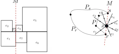
Having studied the nice probabilistic behaviour of parallel circles, we now turn our attention to meridians, i.e. lines in K with a constant width coordinate. We will prove an assertion which is, in a sense, dual to Lemma 6.4: for every meridian M, the expected number of particles crossing M from left to right equals the expected number of particles crossingM from right to left.
Some care needs to be taken before we can make such an assertion, since if our random walk is currently at a vertex x the span T(x) of which (recall that T(x) is a horizontal interval inK) is dissected by M, then we cannot say whether the particle is on the right or left of M. To amend this, we assume that at each step n of our random walk, an additional random experiment is made to choose a random pointPnin the spanT(Zn) of the current positionZn
uniformly among all points inT(Zn), and all these experiments are independent
from each other andZi, i < n, and we think ofPnas the position of our random
walk at stepn. With this assumption in mind, we can now state the following
Lemma 6.6. For every vertex x and every meridian M meeting T(x), the
Proof. To begin with, suppose for simplicity thatM does not dissect any square Re⊂K associated to an edge eincident with x. Thus locally the position of
M is like in the left of Figure 2. By the construction ofT, this implies that for the two vertices r, sofG∗ lying in the faces ofGseparating the edges mapped
to the left of M from those mapped to its right we havew(r) =w(s) =w(M), wherew(M) denotes the common width coordinate of the points inM (Figure 2 right).
x
e1
e1 e2
e2
e3
e3
e4
e4 e5
e5
e6
e6
e7
e7
r s M M
Pr
P
P
[image:22.595.195.397.224.316.2]s
Figure 2: The local situation at a vertexxwhose spanT(x) is dissected by a meridian M in the tiling and the graph.
Now letP be the r–s path in G∗ comprising the set of edgesEr incident
with xon the ‘left’ of M. Recall that the valuesw(r), w(s) where specified by choosing arbitrary paths Pr, Ps from r, srespectively to the reference vertexζ
of G∗, and adding the w(~e) values along such a path. Now note that we can obtain a candidate for Pr by prefixing Ps by P. But since w(r) = w(s), this
implies that P
~e∈Pw(~e) = 0. The definition of the random walk floww now
implies that the net flow intoxalong edges inEris zero. Likewise, the net flow
into xalong the ‘right’ edges El is zero. Our claim that the expected number
of particles crossing M from left to right at xequals the expected number of particles crossing M from right to left now follows from Kirchhoff’s node law (14) and the Sand-bucket Lemma below (brown sand corresponds to particles coming toxfrom the left; shovel them to B if they leavexfrom the right).
It is straightforward to adapt this argument to the general case where M does dissect some squareRe; we leave the details to the reader.
Lemma 6.7(Sand-bucket Lemma). Alice has two (not necessarily equally full)
buckets of sand A and B, where A contains only brown sand and B only white sand. If she puts one shovelful from A to B, mixes arbitrarily, then puts back one shovelful from B to A, then the amount (measured by volume) of white sand in A equal the amount of brown sand in B.
6.3
Convergence of random walk to the boundary
In this section we provide a proof of the almost sure convergence of the image of the trajectory or random walk underT to a point in the boundary C of K which is maybe simpler than the proof of [8]. This proof is the only occasion in this paper where the bounded degree condition cannot be replaced by the weaker (17). LetD:= maxx∈V d(x) be the highest degree inG.
For this, letX be an interval of C, and let ML, MR be the two meridians
corresponding to the endpoints of X. LetL be the set of verticesxsuch that ML intersects T(x), and define R similarly. Note that unlessML, MR happen
to meet some vertex at an endpoint of its span —a possibility we can exclude since there are countably many such meridians—L, Rare the vertex sets of two 1-way infinite paths ofG.
We claim that the expected number of times that our random walk alternates betweenLand Ris finite. This implies that almost surely the number of such alternations is finite, and as this holds for everyX, convergence to the boundary follows.
It is not hard to see that the expected number of times that random walk fromogoes fromLtoRequalsP
x∈LG(o, x) P
y∈Rpxy, where as usualG(o, x)
denotes the expected number of visits tox, andpxydenotes the probability that
random walk from xexits L∪R at a given vertexy ∈R. Thus, we can write the above claim as follows:
P
x∈L,y∈LG(o, x)pxy<∞. (19)
We are going to prove this exploiting the relations between random walks and electrical networks.
Recall thatG(o, x) =h(x)πx(12), and so the above sum equals P
x∈L,y∈Lh(x)πxpxy. The quantityπxpxy was shown in [21] to equal the
‘ef-fective conductance’ Cxy between x and y when the network is finite.
Ef-fective conductance is closely related to energy (recall the physical formula E = I2R = I2/C), and we are going to exploit this fact using an argument similar to the proof of Lemma 5.2. We cannot directly apply the results of [21] as the graph is infinite in our case, however, there is an easy way around this: we can consider an increasing sequence of finite subgraphsH1⊆H2⊆. . .⊆G such thatS
Hn=G, apply the results of [21] toHn and take a limit.
To make this more precise, let pn
xy be the probability that random walk
on Hn from a vertex x ∈ L∩Hn exits (L∪R)∩Hn at y ∈ R∩Hn, and
let Cxyn := πxpnxy. It is a well known property of electrical networks, called
Reyleigh’s monotonicity law, thatCn
xyis monotone increasing withn[32]. Thus
limpn
xy = limCxyn /πx exists. It is now not hard to prove that pxy ≤ limpnxy
using coupling and elementary probabilistic arguments. Thus, to prove (19) it suffices to find a uniform upper bound forP
n:= P
x∈L,y∈LCxyn (where we used
the fact thathis bounded). It is shown in [21] that the above sumP
n equals
the energy En of the harmonic function (or the electric current) on Hn with
boundary conditions 1 at L∩Hn and 0 at R∩Hn. Thus, all we need to do is
to prove that theEn are bounded.
To achieve this, we will invoke the following well known fact: on a finite network, the harmonic function with given boundary conditions minimises en-ergy among all function satisfying the boundary conditions. This means that it suffices in our case to find arbitrary functionsvnwith boundary conditions 1 at
L∩Hn and 0 atR∩Hn and uniformly bounded energiesE(vn). We will do so
by defining a single function v :V →Rwith finite energy E(v) equaling 1 on
Land 0 onR, and lettingvn be its restriction toHn. SinceE(vn)≤E(v), the
E(vn) will indeed be bounded.
by projecting it to the base of K. To check thatE(v)<∞, we will compare E(v) with the energyE(h) of the height functionhwe used in the construction of the tiling. Recall thatE(h) equals the area ofK, which is finite.
Now consider an edge e = wz, set a := |v(w)−v(z)| and recall that the contribution of e to E(v) is (v(w)−v(z))2 = a2. Note that as e joins w to
z, the construction of the tiling implies that T(w), T(z) meet when projected vertically. Combined with our choice of v, this implies that at least one of T(w), T(z) has length at least a/2; assume without loss of generality this is T(z). Now since d(z) is bounded by D, there is at least one edge f = f(e) incident with z such that the corresponding square Rf in the tiling has side
length at least a/2D. This means that the area of Rf is at least a2/(2D)2,
which is a constant times the contributiona2 ofetoE(v). Now note that each edgef ofGcan be considered asf(e) for a bounded number of edgese, namely those sharing an endvertex withf. This easily implies thatE(v) is bounded by a constant timesE(h), and soE(v) is finite sinceE(h) is.
This proves our claim that the expected number of times that our random walk alternates betweenLandR is finite. Applying this to a countable family of pairs Li, Ri such that the corresponding intervals generate the topology of C, and combinining this with the almost sure convergence ofhalong a random walk trajectory, immediately yields
Theorem 6.8. For random walk Zn on G, the intervals T(Zn) almost surely
converge to a point in C.
This allows us to view C as a G-boundary as defined in Section 3: define f :W → Cas follows. For a walkW onGsuch thatT(Wn) converges to a point
p ∈ C, we let f(W) = p; otherwise we let f(W) be a fixed arbitrary point of
C (such walks form a null-set, so it does not really matter). It is easy to check that f is measurable and shift-invariant. Naturally, we define the measuresνz
onC byνz(X) :=µz(f−1(X)), making sure thatf is measure preserving.
Combining Theorem 6.8 with Lemma 6.2, it is an easy exercise to deduce the following fact, already proved in [8], that will be useful later
Corollary 6.9. νo is equal to Lebesgue measure onC.
7
Faithfulness of the boundary to the sharp
har-monic functions
In this section we prove that the boundary Cof the tiling constructed above is faithful to every sharp harmonic function, which we plug into Theorem 1.3 to complete the proof thatC is a realisation of the Poisson boundary of our planar graphG(Theorem 1.1).
Letsbe such a function, fixed throughout this section.