Essays in macroeconomics using microdata

(1)

A Thesis Submitted for the Degree of PhD at the University of Warwick

Permanent WRAP URL:

http://wrap.warwick.ac.uk/110293/

Copyright and reuse:

This thesis is made available online and is protected by original copyright.

Please scroll down to view the document itself.

Please refer to the repository record for this item for information to help you to cite it.

Our policy information is available from the repository home page.

(2)

Essays in Macroeconomics using Microdata

by

Jorge Diego Sol´

orzano Rueda

Thesis

Submitted to the University of Warwick

for the degree of

Doctor of Philosophy

Department of Economics

(3)

List of Tables

2.1 Aggregate frequency of adjustment . . . 24

2.2 Sectoral frequency of adjustment . . . 25

2.3 IV: Frequency of posted price and wage adjustments . . . 28

2.4 IV: Frequency of reference price and wage adjustments . . . 28

2.5 Aggregate absolute size of adjustment . . . 30

2.6 Sectoral absolute size of adjustment . . . 31

2.7 IV: Absolute size of posted price and wage adjustments . . . 32

2.8 IV: Absolute size of reference price and wage adjustments . . . 33

2.9 Best fit by single-sector economy . . . 52

2.10 Appendix: Aggregate frequency of adjustment . . . 55

2.11 Appendix: Sectoral frequency of adjustment . . . 59

2.12 Appendix: IV: Frequency of posted price and wage adjustments . . . 60

2.13 Appendix: IV: Frequency of reference price and wage adjustments . 60 3.1 Region-specific correlations between potential ERPT drivers . . . 83

3.2 Regional pass-through . . . 88

3.3 Industry pass-through . . . 89

3.4 ERPT Determinants . . . 91

3.5 ERPT Determinants for tradables . . . 91

3.6 ERPT Determinants for services . . . 92

3.7 Appendix: ERPT Determinants, after 6 months . . . 96

3.11 Appendix: ERPT Determinants for tradable goods, after 6 months . 98

3.12 Appendix: ERPT Determinants for tradable goods, after 12 months 98

3.13 Appendix: ERPT Determinants for tradable goods, after 18 months 99

(6)

List of Figures

2.1 Inflation, unemployment and GDP in Mexico . . . 11

2.2 Frequency of adjustment: Wages and Earnings . . . 24

2.3 Frequency of adjustment . . . 26

2.4 Distribution of implied durations . . . 27

2.5 Absolute size of adjustment . . . 32

2.6 Absolute size and frequency of adjustment . . . 34

2.7 Distribution of non-zero changes . . . 35

2.8 Multi-sector economy: Posted prices and wages (i) . . . 45

2.9 Multi-sector economy: Posted prices and wages (ii) . . . 46

2.10 Multi-sector economy: Reference prices and wages . . . 47

2.11 Calvo-distribution . . . 53

2.12 Best fit by a single sector economy . . . 53

2.13 Appendix: Frequency of adjustment . . . 56

2.14 Appendix: Absolute size of adjustments . . . 57

2.15 Appendix: Distribution of non-zero changes . . . 58

3.1 Example of price dynamics . . . 73

3.2 Observed regions . . . 74

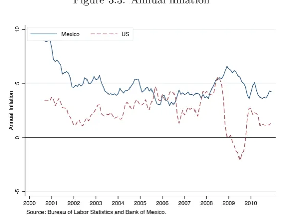
3.3 Annual inflation . . . 74

3.4 MXN Peso - US Dollar Exchange Rate . . . 75

3.5 Regional ERPT at di↵erent time horizons . . . 90

3.6 Industry ERPT at di↵erent time horizons . . . 90

3.7 Appendix: MXN Peso E↵ective Exchange Rate (EER) . . . 93

3.8 Appendix: Regional ERPT after 6 months . . . 94

(7)

Acknowledgments

I would like to thank my supervisors Natalie Chen and Juan Carlos Gozzi and

advisor Huw Dixon. Without their countless comments, reviews and support this

journey would have been impossible.

Big thanks to my family and friends for their endless love and support.

I am also grateful for the partial funding from CONACyT, Banco de Mexico

(8)

Declarations

This thesis is submitted to the University of Warwick in support of my application

for the degree of Doctor of Philosophy. It has been composed by myself and has not

been submitted in any previous application for any degree.

Chapter two is a collaboration with Huw Dixon. It started during my stay

(9)

Abstract

Price and wage setting are key elements in empirical and theoretical macroe-conomic research. In recent years, large micro datasets with millions of observations have expanded our knowledge of wage and price setting practices. Aside from ad-dressing old questions, new salient facts have emerged and have led to improvements, clarifications, criticisms and even new research lines.

One of these new findings in microeconomic research is the high degree of heterogeneity in the behaviour of price and wage setters. This dissertation adds to the research of using large micro datasets to document heterogeneity in price and wage setting, its implications for aggregate dynamics and potential drivers shaping heterogeneous responses.

In chapter one, we provide an introduction to our research on price and wage heterogeneity and provide a short summary of the following two chapters.

In chapter two, we merge three large price and wage micro-datasets at indus-try level and show that the frequency of price and wage adjustments are positively correlated. Furthermore, using a multi-sector DSGE model, we find that adding

heterogeneity in both prices and wages generates small di↵erences in aggregate

dy-namics compared to a model with heterogeneity in only one of them.

In chapter three, we investigate whether price responses to exchange rate shocks, the so-called exchange-rate pass-through, are asymmetric across regions and type of goods. Results suggest heterogeneous pass-through elasticities and that re-gional and industry characteristics play a role in shaping this heterogeneity. For instance, distance to the border, import intensity, price change dispersion and

ex-penditure share a↵ect positively the degree of pass-through; while regional market

density has a negative relationship with pass-through rates.

(10)

Chapter 1

Introduction

Price and wage setting are key elements in empirical and theoretical macroeconomic research. In recent years, large micro datasets with millions of observations have expanded our knowledge of wage and price setting practices. Aside from address-ing old questions, new salient facts have emerged and have led to improvements, clarifications, variations, criticisms and even new research lines.

One of these new findings in microeconomic research is the high degree of heterogeneity in the behaviour of price and wage setters (e.g. Bils and Klenow [2004], Nakamura and Steinsson [2008]). In spite the great deal of heterogeneity in wage and price setting found in large-scale surveys, most studies keep employing simplified frameworks at odds with this heterogeneity (see Smets and Wouters [2003], Gali and Monacelli [2005]). Also, it is not clear what are the drivers of these asymmetric price and wage responses to aggregate shocks (Campa and Goldberg [2005], Le Bihan et al. [2012]).

This dissertation adds to the research of using large micro datasets to docu-ment heterogeneity in price and wage setting, its implications for aggregate dynamics and potential drivers shaping heterogeneous responses.

In chapter two, “Price- and Wage-setting Heterogeneity and Implications in a New Keynesian Economy”, we bring together two strands in the nominal rigidities literature that have been treated independently so far. On the one hand, studies using microdata analysing price adjustments, such as Bils and Klenow [2004]; Naka-mura and Steinsson [2008]; Klenow et al. [2010]; Dixon and Kara [2010]. On the other hand, there is a growing body of literature that focuses on wage setting. See for instance, Barattieri et al. [2014]; Messina and Sanz-de Galdeano [2014]; Le Bihan et al. [2012].

(11)

level. To the author’s knowledge, this is the first study merging price and wage data at such large scale.

Thus, in chapter two we investigate if the frequency of price and wage changes, commonly assumed independent one from each other in macro literature, display similar dynamics. Thus, studying jointly prices and wages new stylised facts emerge from the data: (i) the frequency of price adjustment is positively correlated with the frequency of wage updates across industries; (ii) wage stickiness is greater than the stickiness of reference prices but lower than posted price rigidities; (iii) fre-quency of adjustments is heterogeneous across industries for both prices and wages; (iv) absolute size of price adjustments is heterogeneous for prices but less clear for wages; and (v) frequency and size of adjustments are negatively correlated, not only for prices but for wages as well.

As it has been argued in previous studies, heterogeneous nominal rigidities might have major implications for aggregate dynamics. To that end, a multi-sector DSGE model is used to analyse what are the consequences of the empirical findings above mentioned. Using a time-dependent price and wage setting workhouse frame-work, results suggest that introducing simultaneously heterogeneous price stickiness

and heterogeneous wage stickiness produces small di↵erences in aggregate dynamics

compared to a model where only one, either prices or wages, is heterogeneous while the remaining one is homogeneous in their degree of stickiness. Hence, further com-plicating the model to encompass both sources of heterogeneity at the same time

has little payo↵in terms of real e↵ects and persistency. Though, any heterogeneous

economy generates far more real e↵ects than any homogeneous economy. Therefore,

New Keynesian models abstracting price or wage heterogeneity neglect an important

channel of monetary policy e↵ects.

As a bypass, and since adding heterogeneous nominal rigidities obscures an already complicated model, we revisit the question of what calibration a

homoge-neous economy should follow in order to generate the same real e↵ects as a

hetero-geneous economy. Our analysis suggests that a homohetero-geneous economy calibrated with 3/4 of the weighted mean of frequency of price and wage adjustments generates

the same real e↵ects as the heterogeneous economy.

(12)

hurdles for researchers. Perhaps the early work by Druant et al. [2012] and Bertola et al. [2012] from the Wage Dynamics Network (WDN) represent the first ones to highlight the presence of a relationship between the frequency of price and wage adjustments.

Hence, the above findings call for more work to reconcile price- and wage-setting practices observed at micro level and aggregate dynamics from macro models. Indeed, price setting heterogeneity has being gaining space in New Keynesian lit-erature. Research by Carvalho [2006]; Dixon and Kara [2010]; Kara [2015] stress the importance of taking micro evidence seriously in DSGE modelling. Frameworks incorporating price heterogeneity fit better the data and avoid ad-hoc solutions found in “representative-agent” models. However, these models abstract from wage heterogeneity. Therefore this chapter fills in this gap in the literature.

The second chapter examines price and wage rigidities in the context of a close economy. That is, the role of external factors, such as the exchange rate, in domestic prices and wages is left out in this setup. In the chapter that follows, I move into an open economy setting and, under the fresh lens of microdata, revisit one of the most important topics in international macroeconomics, the so-called Exchange Rate Pass-Through.

In chapter three, “Heterogeneous Exchange Rate Pass-Through: Micro-Level Evidence From Mexico”, the attention is centred at examining the questions: are price responses across regions and type of goods asymmetric to exchange rate shocks? if so, what are the likely factors determining these responses?

The relation between prices and exchange rates is one of the classic topics analysed in international macroeconomics. Though, much of the previous research in this area focuses on the response of headline CPI to exchange rate fluctuations (e.g. Taylor [2000]; Goldberg and Campa [2010]). These studies imply that the pass-through of exchange rates to prices is homogeneous for across the economy. Another strand in the literature focuses on whether pass-through is endogenous to the domestic economy i.e. what drives the degree of pass-through (e.g. Campa and Goldberg [2005]; Fue [2012]).

Chapter three fits right in the heart of these areas of research. Building

on the idea by Goldberg and Campa [2010] that pass-through is di↵erent across

(13)

Estimates suggest that pass-through is incomplete at most horizons, indus-tries and regions. Moreover, great deal of heterogeneity is found in pass-through elasticities. For instance, in the short run, some regions exhibit up to four times larger pass-through rates than other urban areas. These asymmetries are persis-tent also at longer horizons. Furthermore, pass-through pace is heterogeneous as

well. In other words, in some regions exchange rate e↵ects take less than a year,

whereas some other regions take nearly two years. In addition, previous findings arguing that pass-through is heterogeneous across industries is confirmed. On av-erage, for instance, tradable good categories display higher pass-through elasticities than services.

In contrast to most pass-through studies estimating price elasticities only, this research takes a step further and assess local and industry characteristics driv-ing the pass-through responses. We study factors such as distance to the north border, market density, demand conditions, economic development, import

inten-sity, price change dispersion and expenditure share. We find that a↵ecting positively

pass-through elasticities are distance to the border, import intensity, price change dispersion and expenditure share. In contrast, market density has a negative rela-tionship with pass-through rates. Moreover, we find that demand conditions and economic development are positively associated with tradable goods’ pass-through responses.

Hence, results from chapter three has a number of implications for exit-ing pass-through literature. First, we confirm that pass-through is incomplete but not as low as what aggregate data suggests, as argued by other microdata studies like Auer and Schoenle [2016]; Broda and Weinstein [2006]; Gopinath and Rigobon [2008]. Second, our findings welcome further studies regarding heterogeneous price responses to exchange rates. Richer and detailed datasets across locations in a rela-tively homogeneous economy are required in order to shed more light to our results. Third, future research should focus on exchange rate pass-through to the service sector. Chapter three suggests that some service prices go against the common belief that (due to their non-tradable component) they exhibit low pass-through.

(14)

Chapter 2

Price- and Wage-setting

Heterogeneity and Implications

in a New Keynesian Economy

2.1 Introduction

Nominal frictions are introduced in macroeconomic models for addressing real e↵ects

of monetary disturbances. Thus, measures of price and wage stickiness are embedded

in New Keynesian models studying the e↵ects of monetary policy. These measures

are found to have determinant influence on the degree of monetary non-neutrality, inflation persistence and optimal monetary policy rule.

A standard assumption in New Keynesian models is that frequency of price and wage adjustments are set independently (and exogenously) one from the other, despite their obvious relationship through the cost function (marginal cost). Yet, little is known empirically about the joint relationship of price and wage rigidities.

We use monthly economy-wide microdata on consumer prices and wages, merged at industry level, to provide new evidence about the interaction of these two sources of nominal rigidities and its implications in a DSGE model. Our contribution to the empirical study of nominal rigidities is fivefold.

First, we provide evidence that the extensive margin of price adjustments

is positively correlated with the extensive margin of wage changes across di↵erent

(15)

size) of price and wage (non-zero) changes are positively correlated at industry level. However, this relationship turns out to be not robust. Second, we document that reference prices (i.e. excluding transitory prices) are stickier than wages, and wages are stickier than posted prices. Third, frequency of adjustments is heterogeneous across industries for both prices and wages. Forth, absolute size of price adjust-ments is heterogeneous for prices but less clear for wages. And fifth, we confirm that, consistent with state-dependent pricing literature, the frequency and size of adjustments are negatively correlated, not only for prices, but for wages as well.

Then, using a time-dependent price- and wage-setting framework we analyse what are the implications of embedding our extensive margin results in a New Key-nesian economy. In other words, this research use a multi-sector New-KeyKey-nesian

economy where each sector (industry) sets prices and wages `a-la-Calvo. The Calvo

distribution (i.e. set of Calvo pairs- prices, wages) is calibrated from the empirical section summarised above.

We find that heterogeneous nominal rigidities have strong implications in ag-gregate dynamics of the model. For instance, any heterogeneous economy generates

far more real e↵ects than any homogeneous economy with the same mean. However,

no significant di↵erences were found when both prices and wages are heterogeneous

relative to cases in which only one, either prices or wages, is heterogeneous and the remaining one is homogeneous. Also, since adding heterogeneous nominal rigidities obscures an already complicated model, our analysis suggests that a homogeneous economy calibrated with 3/4 of the weighted mean of frequency of price and wage

adjustments generates the same real e↵ects as the heterogeneous economy.

The joint study of wage and price stickiness is relevant in micro-founded New Keynesian DSGE models for numerous reasons.

For instance, macroeconomic models predict that aggregate price level inertia hinges on wage rigidity. As Basu and House [2016] explain surveying wage setting literature, price level responds sluggishly to marginal cost adjustments. As wages are the largest component of the marginal cost (by producing real value added), wage stickiness reinforces price stickiness. Hence, understanding the interactions of price and wage rigidities is essential for aggregate dynamics in macro models.

In addition, the reaction of prices and wages to shocks depends on several factors: (i) the adjustment mechanism generating nominal rigidity (e.g. type of contracts ruling prices and wages behaviour), (ii) the length of the contracts (i.e. the parameters chosen to calibrate the duration of prices and wages) and (iii) the degree of staggering or synchronisation of price and wage adjustments.

(16)

of nominal wage and price stickiness generates a higher persistence of inflation. For instance, if real rigidity is mechanically induced by wage indexation to past

infla-tion, the trade-o↵between output and inflation stabilisation faced by the monetary

authority is worse.

Despite the pivotal role of nominal rigidities in macro modelling, there is no unambiguous evidence on which adjustment rule better characterise price- and wage-setting. The most common assumption in macro literature is that the frequency of price adjustments and the frequency of wage changes are equal (e.g. Erceg et al. [2000]; Gal´ı [2015]). Our purpose in this chapter is to shed light on the interaction of price and wage rigidities and the implications of using a realistic heterogeneous Calvo calibration in an otherwise standard DSGE model.

The analysis begins from two large microdata sets providing monthly price and wage observations across a wide range of industries in Mexico. The first dataset is compiled by the Bank of Mexico (Banco de Mexico) and report price dynamics ob-served at the retail level. Furthermore, we use administrative wage data provided by the Mexican Institute of Social Security (IMSS). Since our administrative wage data neglects the informal labor market, we complement our analysis by using microdata from self-reported earnings data including formal and informal workers. The later survey is gathered by the National Institute of Geography and Statistics (INEGI). Price, wage and earnings data are merged using the North American Industry Clas-sification System (NAICS) and IMSS’s industry clasClas-sification. Our paper exploits the industrial partition in these datasets to study price and wage frequency and size of adjustments.

This chapter is organised as follows, section 2.2 summarises literature related to heterogeneous price and wage rigidities. Section 2.3 describes the micro datasets. Section 2.4 studies the frequency of adjustments. Section 2.5 analyses the absolute size of adjustments. Section 2.6 assess the interaction between frequency and size changes. Section 2.7 shows the complete distribution of price and wage (non-zero) changes. Section 2.8 characterises and summaries aggregate dynamics found in our DSGE model. Lastly, section 2.9 concludes.

2.2 Literature

(17)

Price and wage rigidities have a direct e↵ect of the real e↵ects of monetary policy in DSGE models. Over the last fifteen years, there has been a growing number of empirical studies focusing on agents’ (goods or labor) pricing practices as richer datasets become more available.

Regarding price stickiness, microdata from price indices, namely CPI and PPI, have emerged as an important data source as first studied by Bils and Klenow [2004]. In a similar fashion, and importantly for this research, analysis by Nakamura

and Steinsson [2008] for the US; ´Alvarez et al. [2006] summarising studies from

Euro-area economies; and Bunn and Ellis [2012] and Dixon and Tian [2017] for the UK exploit price indices’ microdata. A clear pattern arises from these studies: prices of some product categories change more frequently than others. This heterogeneous pricing behaviour is confirmed in our CPI micro-dataset for the Mexican economy. Microeconomic evidence on wage stickiness has been also an object of re-search since Taylor. In recent years there has been a renewed interest on studying wage stickiness using higher than annual frequency observations. This research, closely related to studies by Le Bihan et al. [2012] for France, Barattieri et al. [2014] for the US and Sigurdsson and Sigurdardottir [2016] for Iceland, focuses on how rigid nominal wages are. In contrast to the consensus on the price literature, the frequency of wage changes does not display much heterogeneity across industries according to these three studies. Interestingly, our study suggests more pervasive heterogeneity in the frequency of wage adjustments across industries. One

poten-tial reason for the starling di↵erence with previous studies using similar datasets

is that we use a more disaggregated industry classification. Le Bihan et al. [2012], Barattieri et al. [2014] and Sigurdsson and Sigurdardottir [2016] employ three, eight and five sectors respectively, potentially averaging out any heterogeneous behaviour. This dissertation uses 74 industries. Another potential reason could be associated to institutional frameworks. Previous studies have centred at advanced economies, whereas we analyse wage stickiness in an emerging economy.

All in all, heterogeneity in nominal stickiness is a clear pattern of microdata. However, macroeconomic models usually assume identical firms or workers, resetting goods and labor prices at the same (average) frequency of adjustment. Hence, a new generation of DSGE models have been developed to encompass and study the

implications of di↵erent degrees of price and wage stickiness in the economy.

In order to account explicitly for heterogeneity in price and wage sticki-ness, macroeconomic literature has adopted the price-setting framework proposed

by Calvo [1983].1 That is, the economy is divided into a number of sectors and

(18)

each firm (union) changes its price (wage) with a sector-specific frequency of

adjust-ment.2,3

Nonetheless, heterogeneity in wages using Calvo-style rigidities in DSGE models remains scarce. Little heterogeneity observed in the microdata (summarised above for France, US and Iceland) partially explains this gap in the literature. However, this chapter finds asymmetries on the frequency of wage changes across industries in Mexico. Therefore, our DSGE strategy is the first to critically assess the role of heterogeneous wage stickiness on aggregate dynamics. In fact, Kara [2015] suggests that heterogeneous wage stickiness may help to address the large variance of wage mark-up shocks in macroeconomic models as noted by Chari et al. [2009].

Moreover, heterogeneity in price- and wage-setting has been suggested to alleviate New Keynesian models’ shortcomings in failing to reproduce inflation re-sponses found in empirical VARs. See for instance Dixon and Kara [2010] and Kara and Park [2017]. Nontheless, macroeconomic literature has adopted habit forma-tion and (price and/or wage) indexaforma-tion, among other mechanisms, in search of reconciling New Keynesian models and empirical VARs. However, some of these mechanisms are at odds with microdata evidence. In line with Dixon and Kara [2010] and Kara and Park [2017], this chapter advocates that heterogeneity in price-and wage-setting can alleviate shortcomings in terms of the impact price-and persistence of inflation response to monetary policy shocks, while keeping the model consistent with micro evidence.

2.2.1 Mexico as a case study

The Mexican economy provides favourable ingredients for analysing price and wage

dynamics. Mexico adopted a floating exchange rate after the so-calledTequila crisis

in 1994, and from 1999 the Bank of Mexico began a gradual transition to an inflation

targeting regime. Officially announced in 2001, the medium-term inflation target

was set at 3.0% with a 1.0 percentage point variability range. Our analysis starts right after this implementation period by utilising data from 2002.

Likewise, since the adoption of the inflation targeting regime, the Bank of Mexico started to move towards a policy influencing the level of interest rates. From 1999 to 2007, the central bank established borrowed reserves as its key instrument.

Dixon and Kara [2011, 2010] with Taylor-type contracts and Nakamura and Steinsson [2010] using a menu-cost framework.

2_{Another Calvo-style setup reflecting the underlying heterogeneity observed in microdata is the}

Generalised Calvo economy. See Dixon and Le Bihan [2012] and Dixon and Tian [2017] for more.

(19)

Then, from 2008 the Bank of Mexico adopted as its policy instrument the overnight interbank interest rate (tasa de fondeo bancario). Thus, Banxico maintained the interest rate between 7.00% and 8.25% in 2008. In the light of the global financial crisis, Banco de Mexico cut the target rate by 3.75 basis points, from 8.25% to 4.50%, in the first half of 2009, where it remained until March 2013.

Figure 2.1 illustrates key macroeconomic variables in Mexico at time our research centres in. Though, our analysis builds in the use rich micro datasets (and not in aggregate indexes) to add on the study of nominal rigidities.

The study of nominal rigidities using Mexican microdata is not new in the literature. Gagnon [2009] use Mexican price microdata and compare frequency and size of adjustments in episodes of high and low inflation. On the one hand, his findings suggest that the frequency of price changes comoves weakly with inflation when the annual rate of inflation is low (below 15%). On the other hand, the average magnitude of price changes correlates strongly with the inflation rate. Although, this study is not directly comparable to ours since it uses data before 2002, his findings support the a-la-Calvo pricing mechanism used in this paper for the Mexican economy.

(20)

[image:20.595.186.455.130.351.2]

Figure 2.1: Inflation, unemployment and GDP in Mexico

97

98

99

100

101

102

GDP

3

4

5

6

7

Pe

rce

n

ta

g

e

2002q1 2003q1 2004q1 2005q1 2006q1 2007q1 2008q1 2009q1 2010q1

date

Inflation (YoY) Unemployment (Qterly) GDP (HP filtered)

2.3 Data

We merge three large microdata sets. The first is CPI microdata gathered by the Bank of Mexico (Banco de Mexico). This is a confidential dataset contain-ing product-level price dynamics used for CPI calculations. The CPI micro dataset has been used by Gagnon [2009] Gagnon et al. [2013] and Elberg [2016] in somewhat

similar studies. The second data source are administrative wage records from affi

li-ated workers to the Mexican Institute of Social Security (IMSS). Castellanos et al. [2004] use a similar dataset with quarterly observations, whilst our analysis utilises monthly observations. The third microdata set comes from the Mexican National Occupation and Employment Survey (ENOE) conducted by the National Institute of Statistics and Geography (INEGI). This is self-reported survey on earnings and other labor market characteristics from workers in both formal and informal sectors. This survey has been used extensively in the past. For instance Cano-Urbina [2015], Bargain and Kwenda [2011], among others.

(21)

our price data includes industries covered in the CPI only. Hence, we focus on industries in which we observe prices and wages/earnings, 74 in total.

For all aggregate statistics about the frequency and size of price/wage/earnings adjustments, we compute weighted figures across sectors unless we indicate

other-wise. We use Bank of Mexico’s CPI expenditure weights for this purpose.4 Sectoral

level statistics are unweighted averages within the sector.

Data on prices and self-reported earnings are merged according to the North American Industry Classification System (NAICS). Wage data is merged with the former two using IMSS’s industry classification system, which has broad similarities with the NAICS. In what follows, the terms industry and sector are used indistin-guishably. Data sets are described in further detail bellow.

Before we describe each of our datasets in great detail, we believe it is

im-portant to highlight how our price stickiness and wage rigidities comparison di↵ers

relative to previous work.

As summarised in the previous section, most studies analyse price-setting independently from wage-setting. Thus, these studies cannot relate whether price

stickiness hinges on wage stickiness.5 Exceptions are research by Druant et al. [2012]

and Bertola et al. [2012] from the Wage Dynamics Network (WDN) and Carlsson and Skans [2012].

We di↵er from these papers in various directions. Druant et al. [2012] and

Bertola et al. [2012] base their research on qualitative data (interviewing firms’ man-agers about their price-setting practices), whereas our analysis employs quantitative data from actual price and wage quotas. Moreover, Carlsson and Skans [2012] use producer prices on annual basis. In contrast, this research uses monthly data, which is more convenient when measuring adjustment rates. Although Carlsson and Skans [2012] utilise firm (plant) level data, his analysis only comprehends manufacturing industries, while our analysis is through homogeneous goods and services industries. To our knowledge, this is the first paper merging sectoral microdata on prices and wages at such scale. The industry coverage allows addressing the heterogeneity commonly found in previous research on nominal rigidities (Nakamura and Steinsson [2008]; Le Bihan et al. [2012]), and the monthly frequency of observations permits a novel comparison between these two sources of nominal stickiness. Most importantly, studies on wage rigidities are typically available at annual and rarely at quarterly frequency, whereas our analysis studies monthly frequency of adjustments.

4_{Using the industries shares of GDP had only limited impact in our results.}

5_{As Basu and House [2016] argue, wage rigidities might reinforce price stickiness since the largest}

(22)

2.3.1 Price data: CPI microdata

We use monthly price dynamics of individual goods and services observed from June 2002 to December 2010. The number of monthly observations ranges roughly from 53,000 in 2002 to 81,000 in 2010 due to sample extensions throughout the observation period. The CPI dataset classifies priced items into product-categories (equivalent to BLS’s ELIs in the US or ONS’s COICOP classes in the UK), which can be grouped into 4-digits NAICS industries.

We drop product categories whose prices are regulated (e.g. gasoline, elec-tricity, etc) or reported as an index due to its particular treatment by the Bank of Mexico (e.g. landline fee, car insurance, etc). Fresh food is excluded as well due to its stochastic component (e.g. subject to weather conditions or time-varying quality

a↵ecting prices). We also neglect from the analysis the top and bottom 0.5% of

monthly price variations per sector as treatment for outliers. All in all, our price

data represents 72% of Mexico’s CPI.6

Prices are inclusive of sales as long as these sales are conditional on

purchas-ing a spurchas-ingle item (e.g. 3x2 o↵ers are not included). Also, seasonal clearance sales

are not included. In the following section we describe extensively our strategy with respect to sales treatment.

With respect to an item being out of stock, the last e↵ectively observed

price is carried forward. This is the original sampling methodology and our dataset does not flag out stockouts. This procedure is not unusual in the literature (for instance, see Kle and Gopinath and Rigobon [2008]). As noted by Nakamura and Steinsson [2008], this approach would be appropriate if one assumes regular prices are systematically readjusted at the end of stockouts. Furthermore, if an item is replaced by another product, our data reports no price variation. Although this might downward bias our estimates of frequency of changes, product rotation is believed to be around 1% per month.

2.3.2 Wage data: Administrative data

We use administrative records from the Mexican Institute of Social Security (IMSS) from January 2003 to December 2010. These administrative records constitute a census of all formal workers employed in the private sector. It excludes a fraction

of the labor force, namely government employees (affiliated to a di↵erent social

security system) and those employed by the informal sector (not affiliated to any

social security system).

(23)

Our data is a panel of employee clusters observed on a monthly basis. Clus-ters are defined by state, district, county, firm’s size, age, gender, industry and

income level. We observe the wage bill and number of workers within the cluster.7

The original dataset contains on average around 3 million clusters every month. It is worth mentioning that, given the granular characteristics defining each cluster, nearly 80% of clusters have only one or two workers. Hence, a vast majority of clusters actually contains individual wages.

We then define the (log) wage per worker as the ratio of wage bill and the number of workers in that cluster. We only compare monthly wages if and only if the cluster’s size has not changed. This is in order to avoid including false-positive

wage adjustments due di↵erent number of workers in the cluster. If the size of the

cluster varies, we consider it as missing value. Also, since we compare constant size clusters from one month to another, we assume workers in the cluster are the same workers in consecutive months.

We analyse clusters from workers classified as permanent workers only. They represent nearly 93% in our sample. We leave out from the analysis temporal workers as most of these positions are seasonal and/or upon the completion of a specific task. After these specifications, our final dataset contains roughly 2 million clusters per month representing more than 5.4 million workers.

Before moving on to the next data source, there are a number of important issues to highlight regarding IMSS’s administrative records.

First, we do not weight clusters by number of employees. One of the motives is that we cannot observe if all workers in the cluster have indeed experienced a wage adjustment. Additionally, identification of wages changes in big size clusters

is more difficult due to the month-to-month same-size constraint. As estimates are

based on millions of clusters, most of them of relative small size, we opt to compute unweighted statistics within sectors.

Second, workers should not receive less than one minimum wage by law.

This legislation a↵ects the frequency of wage changes for those earning between

the old and new minimum wage. Moreover, the base salary reported to the IMSS

is capped at 25 minimum wages. This celling also a↵ects the frequency of wage

adjustments as every time there is minimum wage update, the reported wage celling is also readjusted, when in fact the worker might not have experienced any wage change. Hence, we carry our analysis excluding workers earning exactly one (4.3%)

7_{Wages in IMSS data are reported in a standardised measure, called base salary. The base}

(24)

or 25 (1.8%) minimum wages.

Third, recent studies base their wage stickiness measures from administrative

wage records as reported by employers. Although misreporting and rounding e↵ects

may still be present, these types of measurement errors might be less of a concern compared to household survey datasets. As argue by Altonji and Devereux [2000], Gottschalk [2005] and Le Bihan et al. [2012], employers provide superior quality data because what they report have direct implications with the fiscal or pension authorities. In fact, Barattieri et al. [2014] stress that, in comparison with the US, other countries have access to administrative data from payroll or tax records, which reduces measurement errors significantly. This is precisely the case for our administrative wage records as reported by the Mexican pension authority IMSS.

We believe our dataset is unlikely to su↵er from measurement errors due to

rounding. On average, 89.5% of our wage observations include the cents paid. Re-garding misreporting, it is in the worker’s interest that employers accurately report her base wage since many of her benefits (e.g. pension, disability insurance, etc.) are proportional to the reported base wage. Although employers have incentives to underreport wages (lowering their social security quotas), the IMSS has the legal status similar to an autonomous fiscal authority. That is, it can engage in legal actions to collect quotas, including seizing firm’s assets, which enhances its ability to enforce the law.

Nonetheless, our wage dataset has three main drawbacks for accurately mea-suring labor costs rigidities.

First, the monthly base wage reported by IMSS is calculated using the wage and time specified on the labor contract. It does not report overtime pay. If the

employee works extra hours and those extra hours are paid at a di↵erent rate, failing

to observe hours worked in our dataset would arguably downward bias our frequency estimates.

Second, our micro-cluster structure may rise to wage trajectories that may not necessarily correspond to the same worker across time. In other words, it could be the case that an employee is substituted by another worker with fairly similar demographics and base salary. Le Bihan et al. [2012] faces a similar issue and tries a number of specifications as robustness checks. However, in our context, if a new

hired has a substantial di↵erent wage and/or have di↵erent demographics (e.g. age),

he or she would fall into a di↵erent micro-cluster. As a result, these instances would

(25)

Third, as base salaries are reported by employers, the IMSS dataset does not

account for between-job wage changes. These cases also a↵ect our frequency of wage

changes if the employee falls into a di↵erent micro cluster, even if he or she is hired

by another firm in the same industry. The use of household surveys (e.g. Barattieri et al. [2014]) or employees’ tax records would allow to calculate between-job wage changes.

2.3.3 Earnings data: Self-reported survey

In order to extrapolate wage rigidities in both formal and informal sectors, we use microdata from the National Occupational and Employment Survey (ENOE). The ENOE is a rotating panel where households are surveyed five times on a quarterly basis. We consider the period from 2005 to 2010 due to methodology changes in the survey.

The ENOE o↵ers job related characteristics (as well as demographics) about

each family member in the household who is 15 years of age or above. We observe individual monthly gross earnings, hours worked, whether the family member is

affiliated to any social security system (e.g. IMSS), as well as employer’s information

such as NAICS industry code, firm’s size, etc.

The surveys’ sample is probabilistic, hence, it provides expansion factors ensuring its representativeness relative to the overall and industry labor market. Thus, after deleting industries in which we do not have price data, our sample comprehends over 60,000 observations, representing nearly 16 million workers, every quarter.

We construct a measure of (log) hourly earnings per worker and we define

an income change as the (log) di↵erence of hourly earnings in consecutive quarters.

It is worth mentioning that data from self-reported earnings might be subject to measurement errors in both variables of interest, earnings and hours worked. We revisit this issue and cleaning procedure in the next section.

2.4 Frequency of price and wage adjustments

In this section, we present statistics on the frequency of price and wage changes in the Mexican economy. We begin by making some precisions on the treatment of sales in the price data, as well as measurement error corrections in the self-reported

earning data. Then, we describe aggregate statistics for our di↵erent data sources,

(26)

First, the literature on nominal rigidities has highlighted that transitory

price changes may substantially bias measures of price stickiness.8 Since our data

lacks sales indicators, we present price statistics using posted prices, as well as reference prices defined as the 3-months modal price. The latter approach, similar toEichenbaum et al. [2011] work, is adopted as a sales filter. Our conclusions do not change if we use 6-months modal prices instead as reported in our Appendix.

Second, our motive for using self-reported earnings data is that it contains data from formal and informal workers. As opposed as our administrative data, containing formal workers only, it provides a complete picture of wage dynamics in Mexico’s labor market. However, literature in labor economics has widely doc-umented measurement errors on self-reported earnings data (e.g. Akee [2011]). In order to clean surveyed data from measurement errors we apply the following clean-ing approach. We first estimate the frequency of price change in our administrative data reported by IMSS. Then, ENOE’s questionnaires ask whether the worker is

an IMSS affiliated or not. We separate these workers into a subsample, then fit

an error band (per industry) in terms of earnings variation such that the frequency of earnings adjustments in this subsample matches the frequency of wage changes (observed in the administrative data). Finally, we impose the same error band to all

workers, including those not IMSS affiliated, and we recalculate earnings’ frequency

of adjustment.9

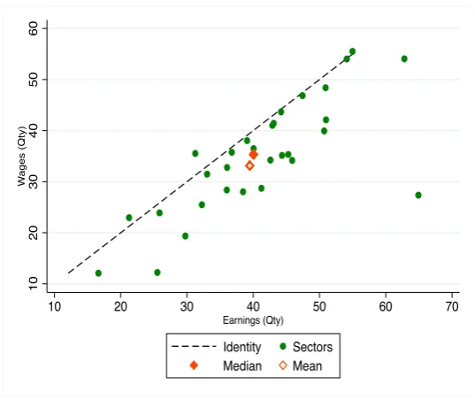
After cleaning our earnings data, wage and earnings frequencies of adjust-ment across industries are depicted in figure 2.2. Remarkably, the positive slope in the graph can be interpreted as industries’ stickiness (relative to other industries) do not change drastically if you consider (or not) both formal and informal workers. Also, since most industries lay below the identity line, it represents that informal workers reset wages slightly more often than employees in the formal sector. This result is likely to prevail if the menu-cost of reseting formal workers’ wage is greater than those in the informal sector, which is likely.

Third, our price and wage datasets contain monthly observations, whereas

8_{For example, Kehoe and Midrigan [2007] and Nakamura and Steinsson [2008].}

9_{Alternative methods have been proposed to alleviate measurement errors in the context of}

(27)

our earnings data is quarterly reported. We use monthly statistics in both the empirical and theoretical part of this chapter. This is a novel feature of our wage data (most studies use annual data and only a handful utilise quarterly observations e.g. Le Bihan et al. [2012]). The expression for transforming self-reported earnings to monthly statistics is

✓_k,qi =✓i_k,m+ ✓i_k,m(1 ✓_k,mi ) + ✓i_k,m(1 ✓_k,mi )2

where✓_k,qi denotes quarterly and✓i_k,mmonthly frequency of adjustment in industry

kfor i= [earnings]. Needless to say, the expression above assumes that the

prob-ability of price adjustment is constant over time, regardless of when was the last

price chance, consistent with the benchmark Calvo model.10

For completeness, we report the corresponding implied duration (in months).

Assuming a constant hazard ✓i

k,m, for i = [price, wage, earnings], we define the

corresponding implied duration as

di_k,m= 1/ln(1 ✓i_k,m)

Finally, aggregate statistics are weighted means/medians across sectors using the 2010 CPI’s weights. All within sector statistics are unweighted statistics.

2.4.1 Aggregate frequency of adjustment

In this section, we summarise the weighted aggregates of the frequency of price,

wage and earnings adjustments. We also present the implied durations, di_k,m, as

defined above. These aggregate statistics are reported in Table 2.1.

Prices

The first and second row in table 2.1 report estimates for posted and reference prices. The median frequency of posted prices is 13.16%, whereas for reference prices it drops to 10.39%. The median implied duration is 7.09 and 9.12 months for posted and reference prices respectively. The mean is 19.94% for posted prices and 13.84% for reference prices. That is, around a 45% and 30% increase with respect to their medians respectively. This implies some skewness in the distribution of the frequency of price changes by sectors.

10_{Alternatively, we could have calculated the actual duration-dependent reset probabilities as}

(28)

Unfortunately there is no other study using the same dataset for cross-checking our estimates. The closest study is by Gagnon [2009] who uses data from 1994 until 2002 and reports an unweighted frequency of price adjustment of 43.4% including sale prices. It is not surprising that our estimates are below this figure as theTequila crisis began in the eve of 1994.

Compared to studies from other developed economies, Mexico displays a sim-ilar degree of price stickiness. For instance, the median frequency of price changes is 19.3% including sales and 8.9% excluding sales in the US as reported by Nakamura and Steinsson [2008]. For the UK, Dixon and Tian [2017] exclude sales and substi-tutions and find a slightly higher statistic of 14%. Moreover, Dixon and Le Bihan [2012] study french data and calculate a weighted mean frequency of 19% including sales.

Wages and earnings

With respect of wages and earnings, aggregate statistics are summarised in the third and fourth row of table 2.1. As highlighted above, our surveyed data contains a sample of formal and informal workers, while the administrative dataset contains the universe of formal employees only with the advantage of less measurement errors. The weighted median frequency of wage adjustments is 14.31%, whereas for self-reported earnings it is 18.81%. Implied duration is about 5 or 6 months depending the data used.

Using Mexican data, Castellanos et al. [2004] report that nearly 95% of wages change every year in 2000q4. Since the authors do not weight sectors and instead they use simple averages, our monthly frequency of adjustment is not strictly comparable to their figure.

Compared to the US or Europe, the Mexican labour market exhibits anal-ogous wage stickiness to Europe. For instance, wage stickiness in France is about 14.7% as documented by Dixon and Le Bihan [2012]. In contrast, Barattieri et al. [2014] report higher wage rigidity in the US, around 9.9% wage changes per month.

2.4.2 Sectoral frequency of adjustment

In this section we describe the relationship between sectoral price, wage and earn-ings frequencies of adjustments. The complete set of industries and frequency of adjustments are listed in table 2.2.

Table 2.2 gives a good idea about the heterogeneous price and wage setting

(29)

nominal rigidities research (e.g. Bils and Klenow [2004]). For instance, only 3% of Parking vehicle services fees vary every month on average, while around 45% of

Grains and seeds related prices change in a month. Also, the e↵ect of transitory prices varies dramatically by industries. A good example are the two measures

of frequency of adjustments for Fat and oil goods: 48% when considering posted

prices and only 19.64% when using reference prices. This e↵ect is less prevalent

in Domestic personnel fees, for instance, which exhibit 3.41% and 3.09% rates of change for posted and reference prices respectively.

Strikingly, the frequency of wage adjustments for most sectors is greater than the frequency of adjustments of reference price, but lower than posted prices.

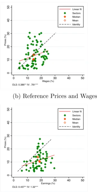
We depict the industries’ frequency of adjustments of posted prices and wages in figure 2.3a. A simple OLS regression gives a correlation of 0.586** between sectoral price and wage frequencies. The positive correlation holds after removing transitory prices by using reference prices. The correlation between the frequency of adjustments of reference prices and wages is 0.336*** as depicted in figure 2.3b.

Looking at price rigidities on the vertical axis of figures 2.3a and 2.3b, the e↵ect of

transitory prices is clear.

The positive relationship prevails across our di↵erent metrics of frequency of

adjustments. For instance, posted prices against earnings (figure 2.3c and correlation 0.539*), reference prices versus earnings (figure 2.3d and correlation 0.297*). Results using 6 months reference prices or wages without floors or caps are essentially the same and can be found in the Appendix.

To our knowledge this is the first paper documenting this positive relation-ship using both price and wage microdata. Druant et al. [2012] highlight similar findings based on qualitative questionnaire answers. In line with our results, the authors report that 73% of firms change wages and prices at a somewhat compara-ble frequency; and 40% of managers acknowledge the existence of some relationship between the time of repricing and wage updates.

In line with previous studies analysing nominal rigidities, we plot the dis-tribution of implied duration across sectors in figure 2.4. These implied durations

are calculated using the expression fordi_k,m as defined above and the frequencies of

(30)

Endogeneity

Several studies have explored whether industries’ heterogeneity in market and/or

cost structure explains why price flexibility di↵ers substantially across industries.

This chapter focuses on the latter, cost structure.11 Previous work studying

the correlation between input shares and the frequency of price adjustments have found an inverse relationship between the degree of labor intensity and price sticki-ness. See, for instance, Peneva [2011] with US consumer prices; and using producer

price data ´Alvarez et al. [2010] for Spain, Dossche and Cornille [2006] for Belgium

and Bertola et al. [2012] for Euro area economies. Results from these studies are only explained in case there is a causal relationship between wage and price stick-iness. Intuitively, the idea of these studies is to link the volatility of labour price (weighted by its factor intensity) and the frequency of price changes. However, these studies are not able to show that relationship as they lack wage data.

Indeed, one of the main conclusions drawn from the IPN is indeed that wage persistence is an important factor behind price stickiness in the Euro area

as summarised by Altissimo et al. [2006].12 Similarly, Peneva [2011] argue that it

is possible that a significant amount of wage rigidity, along with the heterogeneity in labor intensity, play an important role in the heterogeneity of price rigidities.

´

Alvarez et al. [2010] state that given the low frequency of wage changes, we expect more labour intensive industries to carry out price revisions less frequently. Druant et al. [2012] use qualitative data from the WDN and establish that firms reset prices roughly at the same time as wage adjustments.

A novel contribution of this chapter is precisely to relate measures of price and wage stickiness across industries using quantitative data. Using better quality data, this chapter critically examines if wage rigidities generate price rigidities.

Following ´Alvarez et al. [2010] and Dossche and Cornille [2006], we regress

the sectoral frequencies of price adjustments on sectoral frequencies of wage changes and additional determinants suggested by economic theory.

As the frequency of wage changes might be contemporaneously determined by

the frequency of price adjustments, we cannot exclude that our regression su↵er from

an endogeneity problem, which leads to biased and inconsistent estimates. Hence, in order to control for this issue we rely on Instrumental Variable (IV) estimation.

11_{Carlton (1986) and Caucutt et al. (1999), Bils and Klenow (2004) and Klenow and Malin}

(2011) focus on market structure determining the degree of price flexibility.

12_{The relevance of understanding the relationship between wages and prices stickiness found from}

(31)

We think of a linear model of the form

F P Ak = F W Ak+"k

with the frequency of posted price adjustments in sector k (F P Ak) as dependent

variable and the frequency of wage adjustments (F W Ak) as independent variable.

In the presence of endogeneity bias,E(F W A")6= 0, we need an instrument that is

correlated withF W A, but not withF P A.13

We propose the share of minimum wage workers per industry as our instru-ment. The intuition behind our instrument is as follows. The minimum wage in

Mexico changes only once a year.14 _{Now, suppose all workers in a given industry}

earn exactly one minimum wage. In this hypothetical industry, all wages would be adjusted when the minimum wage changes. Since we use monthly data, this means that we would observe a wage change every twelve months. In other words, if 100% of workers earn the minimum wage, we would expect to have a frequency of adjustment equal to one twelfth. Similarly, as the share of minimum wage workers decreases per industry, the stochastic component of wage determination kicks in, presumably leading to more frequent wage adjustments. Although one might argue the opposite (that is, as the share of minimum wage workers decreases per industry, wage determination leads to less frequent than once a year wage adjustments), our wage statistics presented above suggest wages are reset, in general, slightly more frequently than once a year. Hence, we assume the fraction of workers getting the

annual minimum wage increase in a given industry a↵ects the frequency of wage

changes in such industry, which in turn determines the frequency of price adjust-ments.

We calculate the share of workers earning up to 1.5 times the minimum wage, per industry, from our administrative data only. The main reasons to neglect informal workers come from the similarities with formal workers found and described in the previous section.

Table 2.3 reports results from our IV approach when treating posted prices

as our dependent variable. The coefficient under the IV estimation in column 2

is nearly double the standard OLS regression in column 1, confirming endogeneity

13_{It is worth noticing that our approach is to focus on the e}_↵_{ects of wages on prices, and not the}

opposite. The intuition is that goods’ prices in a given industry rely heavily on wages (costs) in such industry. On the other hand, wages in certain industry depend on the aggregate price level across industries. Given the structure of our dataset, we centre our attention in the wage on price

e↵ects.

14_{This is the case at least during our observation period. More recently, there have been years}

(32)

issues. Diagnostic statistics, such as the F-statistic or the minimum eigenvalue, in column 2 discard concerns of weak instrumentation.

Given the limited number of industries in our sample, we can only take our

analysis in few di↵erent directions. First, we consider an alternative instrument,

namely the industry labor share. The intuition here is that as labour share becomes larger, unions or households have more bargaining power on wage adjustments,

which in turn determines prices (only after a↵ecting wages). The result of this

approach is shown in column 3 of table 2.12 in the appendix. Although our coefficient

of interest is positive and statistically significant (three times larger than the simple OLS), labour share turns out to be a weak instrument for FWA as shown from the F-statistic. Column 4 reports results from a 2SLS using both instruments. Not surprisingly the correlation between FPA and FWA remains positive and statistically significant.

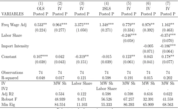
Second, we use three less parsimonious models controlling for additional

co-variates with our original instrument. These regressors are likely to a↵ect pricing

decisions as well: labor share (proxy for technology) or import intensity (proxy for exchange rate fluctuations) or both in columns 3, 4 and 5 respectively in table 2.3. In all these cases we also find a positive and statistically significant relationship

between FPA and FWA.15The F-statistic and the minimum eigenvalue do not seem

to vary much compared to those in column 2.

We then repeat the same econometric strategy but now using as a dependent variable the frequency of adjustments of reference prices. Results are reported in table 2.4. Although the correlation is about half compared to that estimated with posted prices, it remains positive and statistically significant.

All in all, we find enough evidence to conclude that the frequency of price changes and the frequency of wage adjustments are positively correlated. That is, sectors changing more often their prices are also updating their wages more frequently. This correlation ranges approximately from 0.5 to 1. Consistent with price stickiness literature, this result implies heterogeneity in the frequency of wage variations, as it is observed in our data.

15_{Druant et al. [2012] and Dias et al. endorse the existence of a relationship between wage and}

price rigidity to the labor intensity characteristics of sectors. In their view, prices are more flexible when labor costs account for a lower fraction of firms’ total costs. We obtain a similar result by

finding a negative coefficient in columns 5 and 7 in table 2.3. Though, as shown before, labour

(33)

Figure 2.2: Frequency of adjustment: Wages and Earnings

10

20

30

40

50

60

W

a

g

e

s

(Q

ty)

10 20 30 40 50 60 70

Earnings (Qty)

Identity Sectors

[image:33.595.186.455.128.354.2]

Median Mean

Table 2.1: Aggregate frequency of adjustment

Median Mean

Frequency Implied Duration Frequency Implied Duration

(%) (Months) (%) (Months)

Posted Prices 13.16 7.09 19.94 4.50

Reference P (3m) 10.39 9.12 13.84 6.71

Wages 14.31 6.48 14.42 6.42

Earnings 18.81 4.80 17.55 5.18

Calvo parameters around the globe (monthly equivalent): All prices: US 19.3%, France 19%;

(34)

[image:34.595.166.469.134.734.2]

Table 2.2: Sectoral frequency of adjustment

Frequency of Adjustment

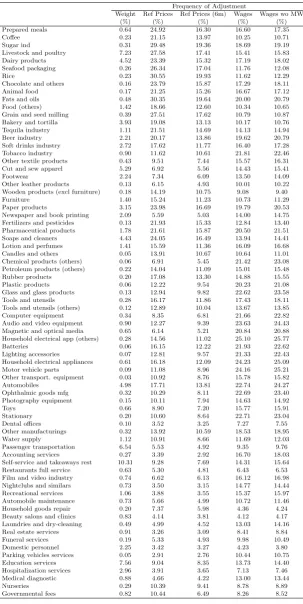
Weight Posted Prices Ref Prices Wages Earnings

(%) (%) (%) (%) (%)

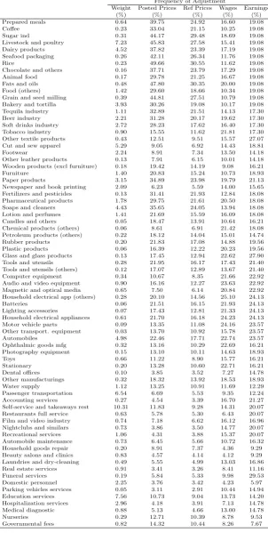
Prepared meals 0.64 39.75 24.92 16.60 19.08

Co↵ee 0.23 33.04 21.15 10.25 19.08

Sugar ind 0.31 44.17 29.48 18.69 19.08

Livestock and poultry 7.23 45.83 27.58 15.41 19.08

Dairy products 4.52 37.82 23.39 17.19 19.08

Seafood packaging 0.26 42.11 26.34 11.76 19.08

Rice 0.23 49.66 30.55 11.62 19.08

Chocolate and others 0.16 37.71 23.79 17.29 19.08

Animal food 0.17 29.78 21.25 16.67 19.08

Fats and oils 0.48 47.80 30.35 20.00 19.08

Food (others) 1.42 29.60 18.66 10.34 19.08

Grain and seed milling 0.39 44.81 27.51 10.79 19.08

Bakery and tortilla 3.93 30.26 19.08 10.17 19.08

Tequila industry 1.11 32.89 21.51 14.13 17.30

Beer industry 2.21 31.28 20.17 19.62 17.30

Soft drinks industry 2.72 28.23 17.62 16.40 17.30

Tobacco industry 0.90 15.55 11.62 21.81 17.30

Other textile products 0.43 12.51 9.51 15.57 27.07

Cut and sew apparel 5.29 9.05 6.92 14.43 18.81

Footwear 2.24 8.91 7.34 13.50 14.18

Other leather products 0.13 7.91 6.15 10.01 14.18

Wooden products (excl furniture) 0.18 19.42 14.19 9.08 16.21

Furniture 1.40 20.83 15.24 10.73 18.93

Paper products 3.15 34.89 23.98 19.79 21.13

Newspaper and book printing 2.09 6.23 5.59 14.00 15.65

Fertilizers and pesticides 0.13 31.41 21.93 12.84 18.08

Pharmaceutical products 1.78 29.75 21.61 20.50 18.08

Soaps and cleaners 4.43 35.65 24.05 13.94 18.08

Lotion and perfumes 1.41 21.69 15.59 16.09 18.08

Candles and others 0.05 18.47 13.91 10.64 16.21

Chemical products (others) 0.06 8.61 6.91 21.42 18.08

Petroleum products (others) 0.22 18.12 14.04 15.01 14.74

Rubber products 0.20 21.83 17.08 14.88 19.56

Plastic products 0.06 16.39 12.22 20.23 19.56

Glass and glass products 0.13 17.45 12.94 22.62 27.90

Tools and utensils 0.28 21.95 16.17 17.43 21.40

Tools and utensils (others) 0.12 17.07 12.89 13.67 21.40

Computer equipment 0.34 10.67 8.35 21.66 22.92

Audio and video equipment 0.90 16.16 12.27 23.63 22.92

Magnetic and optical media 0.65 7.50 6.14 20.84 22.92

Household electrical app (others) 0.28 20.10 14.56 25.10 24.13

Batteries 0.06 21.51 16.15 21.93 24.13

Lighting accessories 0.07 17.43 12.81 21.33 24.13

Household electrical appliances 0.61 21.70 16.18 24.23 24.13

Motor vehicle parts 0.09 13.35 11.08 24.16 23.57

Other transport. equipment 0.03 13.70 10.92 15.78 23.57

Automobiles 4.98 22.46 17.71 22.74 23.57

Ophthalmic goods mfg 0.32 13.16 10.29 22.69 16.21

Photography equipment 0.15 13.10 10.11 14.63 18.93

Toys 0.66 11.22 8.90 15.77 16.21

Stationary 0.20 13.28 10.60 22.71 16.21

Dental offices 0.10 3.85 3.52 7.27 14.78

Other manufacturings 0.32 18.32 13.92 18.53 18.93

Water supply 1.12 13.25 10.91 11.69 12.29

Passenger transportation 6.54 6.69 5.53 9.35 12.24

Accounting services 0.27 4.54 3.39 16.70 21.27

Self-service and takeaways rest 10.31 11.83 9.28 14.31 20.07

Restaurants full service 0.63 5.78 5.30 6.43 20.07

Film and video industry 0.74 7.18 6.62 16.12 16.96

Nightclubs and similars 0.73 3.86 3.50 14.77 20.07

Recreational services 1.06 4.31 3.88 15.37 20.07

Automobile maintenance 0.73 6.45 5.66 10.72 16.32

Household goods repair 0.20 8.91 7.37 4.36 9.29

Beauty salons and clinics 0.83 4.57 4.14 4.12 9.29

Laundries and dry-cleaning 0.49 5.55 4.99 13.03 16.86

Real estate services 0.91 3.41 3.26 8.41 11.16

Funeral services 0.19 5.84 5.33 9.98 29.53

Domestic personnel 2.25 3.76 3.42 4.23 5.97

Parking vehicles services 0.05 3.11 2.91 10.44 14.94

Education services 7.56 10.73 9.04 13.73 14.20

Hospitalization services 2.96 4.18 3.91 7.13 14.78

Medical diagnostic 0.88 5.13 4.66 13.00 14.78

Nurseries 0.29 12.71 10.39 8.78 9.53

(35)

[image:35.595.325.484.256.569.2]

Figure 2.3: Frequency of adjustment

0

10

20

30

40

50

Pri

ce

s

(%

)

0 10 20 30 40 50

Wages (%)

Linear fit Sectors Median Mean Identity

OLS: 0.533* IV: 1.16**

(a) Posted Prices and Wages

0

10

20

30

40

50

Pri

ce

s

(%

)

0 10 20 30 40 50

Wages (%)

OLS: 0.386** IV: .781***

(b) Reference Prices and Wages

0

10

20

30

40

50

Pri

ce

s

(%

)

0 10 20 30 40 50

Earnings (%)

OLS: 0.662* IV: 1.97***

(c) Posted Prices and Earnings

0

10

20

30

40

50

Pri

ce

s

(%

)

0 10 20 30 40 50

Earnings (%)

OLS: 0.437** IV: 1.32***

(36)

Figure 2.4: Distribution of implied durations

0

5

10

15

20

25

30

35

Sh

a

re

(%

)

0 3 6 9 12 15 18 21 24 27 30 33 36

Months

(a) Posted Prices

0

5

10

15

20

25

30

35

Sh

a

re

(%

)

0 3 6 9 12 15 18 21 24 27 30 33 36

Months

(b) Reference Prices

0

5

10

15

20

25

30

35

Sh

a

re

(%

)

0 3 6 9 12 15 18 21 24 27 30 33 36

Months

(c) Wages

0

5

10

15

20

25

30

35

40

45

Sh

a

re

(%

)

0 3 6 9 12 15 18 21 24 27 30 33 36

Months

(37)

Table 2.3: IV: Frequency of posted price and wage adjustments

(1) (2) (3) (4) (5)

OLS IV IV IV IV

VARIABLES Posted P Posted P Posted P Posted P Posted P

Freq Wage Adj 0.533** 0.964*** 0.779** 0.978** 1.162**

(0.224) (0.277) (0.334) (0.392) (0.463)

Labor Share -0.246*** -0.374***

(0.058) (0.070)

Import Intensity -0.005 -0.186***

(0.071) (0.064)

Constant 0.107*** 0.042 0.123** 0.043 0.178**

(0.038) (0.043) (0.061) (0.041) (0.077)

Observations 74 74 74 74 74

R-squared 0.048 0.017 0.191 0.015 0.202

IV MW Sh MW Sh MW Sh MW Sh

Adj R2 0.534 0.598 0.616 0.622

Robust F 48.939 67.257 32.391 41.558

Min Eig 84.554 86.393 65.909 68.563

Robust standard errors in parentheses

*** p<0.01, ** p<0.05, * p<0.1

Table 2.4: IV: Frequency of reference price and wage adjustments

(1) (2) (3) (4) (5)

OLS IV IV IV IV

VARIABLES Ref P Ref P Ref P Ref P Ref P

Freq Wage Adj 0.386*** 0.675*** 0.564*** 0.673*** 0.781***

(0.134) (0.170) (0.201) (0.236) (0.275)

Labor Share -0.148*** -0.220***

(0.035) (0.041)

Import Intensity 0.001 -0.105***

(0.042) (0.038)

Constant 0.075*** 0.031 0.080** 0.031 0.111**

(0.022) (0.026) (0.036) (0.025) (0.045)

Observations 74 74 74 74 74

R-squared 0.070 0.031 0.208 0.031 0.208

IV MW Sh MW Sh MW Sh MW Sh

Adj R2 0.534 0.598 0.616 0.622

Robust F 48.939 67.257 32.391 41.558

Min Eig 84.554 86.393 65.909 68.563

Robust standard errors in parentheses

(38)

2.5 Absolute size of price and wage adjustments

We present in this section features from the distribution of the absolute size of price and wage adjustments (given a non-zero change). Similarly as in the previous section, we describe aggregate weighted statistics and we then provide a sectoral comparison between prices and wages. We neglect from this section earnings data

due to measurement errors.16

Prices’ and wages’ absolute size of (non-zero) adjustments of are important for a number of reasons. First, we consider absolute values because we do not want positive and negative changes to average out. Second, it is well stablished that both goods’ and labour’s prices often remain fixed for a number of periods, followed by a not negligible variation. Thus, we neglect the overwhelming number of zeros in our sample. In other words, these are the absolute size of adjustments conditional on a price/wage change. Third, from the theoretical point of view, the size of the adjustment is often viewed as indicative on how and when cost inflation pressure is released. In other words, how willing are firms to deviate from their optimal price i.e. the so-called S,s area.

2.5.1 Aggregate size of adjustment

Table 2.5 reports the aggregate weighted median and mean of the absolute size of adjustment for posted and reference prices, as well as wages. The aggregate median is calculated by first calculating the unweighted mean of price and wage changes in absolute terms within each sector; and then taking a weighted median across sectors using CPI expenditure weights. Likewise, the aggregate mean is computed as the weighted mean across sectors from unweighed sectoral means.

The di↵erences between the mean and median for our two di↵erent measures

of prices changes is small. For posted prices the median is 7.16% and the mean is 7.21%. In the case of reference prices 8.13% and 8.00% are the median and mean respectively. The fact that posted prices’ first moments are smaller than their reference prices’ counterparts implies that transitory discounts (included in our posted prices measure) are smaller, on average, than non-transitory price variations. The median and mean of the absolute size of wage adjustments are almost identical, 3.25% and 3.26%. Noticeably, these values are very close to the inflation target set by the Mexican Central Bank at 3%; and less than the average increase

16_{Fitting an error band as in the frequency of adjustment section is a good bypass for controlling}