http://wrap.warwick.ac.uk/
Original citation:
Doan, Xuan Vinh, Li, Xiaobo and Natarajan, Karthik . (2015) Robustness to dependency in portfolio optimization using overlapping marginals. Operations Research, 63 (6). pp. 1468-1488.
http://dx.doi.org/10.1287/opre.2015.1424
Permanent WRAP url:
http://wrap.warwick.ac.uk/73640
Copyright and reuse:
The Warwick Research Archive Portal (WRAP) makes this work of researchers of the University of Warwick available open access under the following conditions. Copyright © and all moral rights to the version of the paper presented here belong to the individual author(s) and/or other copyright owners. To the extent reasonable and practicable the material made available in WRAP has been checked for eligibility before being made available.
Copies of full items can be used for personal research or study, educational, or not-for-profit purposes without prior permission or charge. Provided that the authors, title and full bibliographic details are credited, a hyperlink and/or URL is given for the original metadata page and the content is not changed in any way.
A note on versions:
The version presented here may differ from the published version or, version of record, if you wish to cite this item you are advised to consult the publisher’s version. Please see the ‘permanent WRAP url’ above for details on accessing the published version and note that access may require a subscription.
Authors are encouraged to submit new papers to INFORMS journals by means of a style file template, which includes the journal title. However, use of a template does not certify that the paper has been accepted for publication in the named jour-nal. INFORMS journal templates are for the exclusive purpose of submitting to an INFORMS journal and should not be used to distribute the papers in print or online or to submit the papers to another publication.
Robustness to Dependency in Portfolio Optimization
using Overlapping Marginals
Xuan Vinh Doan
DIMAP and ORMS Group, Warwick Business School, University of Warwick, Coventry, CV4 7AL, United Kingdom, [email protected]
Xiaobo Li
Industrial and Systems Engineering, University of Minnesota, Minneapolis, MN 55455, [email protected]
Karthik Natarajan
Engineering Systems and Design, Singapore University of Technology and Design, 8 Somapah Road, Singapore 487372, natarajan [email protected]
In this paper, we develop a distributionally robust portfolio optimization model where the robustness is across
different dependency structures among the random losses. For a Fr´echet class of discrete distributions with
overlapping marginals, we show that the distributionally robust portfolio optimization problem is efficiently
solvable with linear programming. To guarantee the existence of a joint multivariate distribution consistent
with the overlapping marginal information, we make use of a graph theoretic property known as the running
intersection property. Building on this property, we develop a tight linear programming formulation to find
the optimal portfolio that minimizes the worst-case Conditional Value-at-Risk measure. Lastly, we use a
data-driven approach with financial return data to identify the Fr´echet class of distributions satisfying the
running intersection property and then optimize the portfolio over this class of distributions. Numerical
results in two different datasets show that the distributionally robust portfolio optimization model improves
on the sample-based approach
Key words: distributionally robust optimization, portfolio optimization, overlapping marginals
History: This paper was first submitted in May 2013, revised twice in April 2014 and December 2014, and
finally accepted in August 2015.
1. Introduction
Optimization under uncertainty is an active research area with several interesting applications in
the area of risk management. An example of a risk management problem is to choose a portfolio
of assets with random returns such that the joint portfolio risk is minimized while a fixed level of
expected return is guaranteed. Markowitz (1952) was the first to model this problem using variance
as the risk measure. Several alternative risk measures have been proposed since for this problem.
Value-at-Risk (VaR) and Conditional Value-at-Risk (CVaR) are two such popular risk measures
(see, for example, Jorion (2001) and Rockafellar and Uryasev (2000)). However even assuming that
the joint distribution of the random returns is known, the calculation of VaR and CVaR for a
given portfolio involves multidimensional integrals, which can be computationally challenging. For
discrete distributions, the computation of these risk measures requires the consideration of all the
support points of the joint distribution. The number of support points of the joint distribution
can however be exponentially large in comparison to the number of support points of the marginal
distributions. For example, the problem of computing the probability that a sum of independent
but not necessarily identically distributed integer random variables is less than a given number is
known to be #P-hard (see Kleinberg et al. (2000)). Furthermore, if the assumed joint distribution
does not match the actual distribution, the optimal portfolio allocation might perform poorly in
out of sample realizations.
One popular approach to address this issue is that instead of assuming a complete joint
distri-bution for the random returns of the risky assets, only reliable partial distridistri-butional information
is used. Given limited distributional information, it is then natural to calculate the worst case
bounds for the VaR and CVaR measures and optimize the worst case bounds. Several models
have been proposed to capture the uncertainty (or ambiguity) in distributions. This includes the
class of distributions with information on the first and second moments (see El Ghaoui et al.
(2003), Delage and Ye (2010), Natarajan et al. (2009a), Zymler et al. (2013)), the Fr´echet class of
(1979), Denuit et al. (1999)) and the Fr´echet class of distributions with information on the
mul-tivariate marginals of non-overlapping subsets of asset returns (see Doan and Natarajan (2012),
Garlappi et al. (2007), R¨uschendorf (1991)). In this paper, we adopt a more general representation
of distributional uncertainty where the multivariate marginals possibly overlap with each other.
1.1. Problem Setup
Throughout this paper, we use standard letters such asx to denote scalars, bold letters such asx
to denote vectors, tilde notation such as ˜cto denote random variables and the calligraphic notation
such asC to denote sets with C= size(C).
Let˜cbe aN-dimensional random vector whereN ={1, . . . , N}is the set of indices of the random
vector. Consider a convex piecewise linear function of the random vector defined as:
ϕ(˜c) , max j∈M
˜
cTaj+bj
, (1)
where the maximum is over the set of affine functions of the random vector indexed by M=
{1, . . . , M} with aj∈ <N, b
j ∈ < and ˜c T
aj =P
i∈Nc˜iaji. Let θ denote the N-dimensional joint
distribution ofc˜. Associated with (1), is the evaluation of its expected value:
Eθ
max j∈M
˜
cTaj+bj
, (2)
and a stochastic optimization problem of the form:
min x∈X Eθ
max j∈M
˜
cTaj(x) +bj(x)
, (3)
where aj(x) and bj(x) are assumed to be affine functions of the decision vector x that is chosen
from a feasible region X. Portfolio optimization with the CVaR measure lies within the scope of
the stochastic optimization problem (3). To see this, let ˜ci denote the random loss of theith asset.
The total portfolio loss is then ˜cTx where xi is the allocation in the ith asset. The CVaR of the
portfolio for a given risk level α∈(0,1) is defined as (see Rockafellar and Uryasev (2000, 2002)):
CVaRθα ˜c T
x
, min
β∈< β+
1 1−αEθ
"
˜
cTx−β
+#!
where y+= max{0, y}. The problem of finding the portfolio x∈ X that minimizes the CVaR is
then formulated as:
min
x∈X,β∈< β+
1 1−αEθ
"
˜
cTx−β
+#!
.
Portfolio optimization with the VaR measure is however not an instance of problem (3) due to the
inherent non-convexity of VaR. It is possible though to develop convex approximations to the VaR
measure using the CVaR measure (see Nemirovski and Shapiro (2006)).
In the distributionally robust optimization setting, θ is not known exactly except that it lies in
a set of distributions denoted by Θ. Then, it is natural to calculate upper and lower bounds on
the expected value Eθ[ϕ(˜c)]. In this paper, we restrict our attention to finding the tightest upper
bound on the expected value of the piecewise linear convex function in (2):
sup θ∈Θ
Eθ
max j∈M
˜
cTaj+bj
. (4)
The corresponding distributionally robust counterpart of (3) is:
min
x∈X supθ∈Θ Eθ
max j∈M
˜
cTaj(x) +bj(x)
, (5)
where the optimal decisionx∈ X is identified for the worst-case distribution in the set Θ.
1.2. Fr´echet Class of Distributions
One of the early results in multivariate bounds is the work of Fr´echet (1940), Fr´echet (1951)
who evaluated bounds on the cumulative distribution function of a random vector given only the
marginal distributions of the random variables. The class of joint distributions with fixed marginal
distributions is referred to as the Fr´echet class of distributions and the bounds are referred to as
Fr´echet bounds. In this paper, we develop a new class of Fr´echet bounds and apply it to to solve
distributionally robust optimization problems.
Given a set N, let E ={J1, . . . ,JR} ⊆2N be a cover of the set N, i.e.,
S
r∈RJr=N, where
R={1, . . . , R}. Assume that there is no inclusion among the subsets, i.e., Jr*Js for any r6=s.
• Partition:E is a partition or a non-overlapping cover if for anyr6=s,Jr∩ Js=∅. The cover:
E={{1},{2}, . . . ,{N}},
is called thesimple partition and forms the basic Fr´echet class of distributions. When some of the
subsets consist of more than one random variable, the partition is referred to as a non-overlapping
multivariate marginal cover. An example of such a partition is:
E={{1,2},{3,4, . . . , N}}.
• Star cover:Let{I0,I1, . . . ,IR}be a partition ofN. ThenE is a star cover ifJr=Ir∪ I0 for
all r∈ R. The star cover:
E={{1,2},{1,3}, . . . ,{1, N}},
is called thesimple star cover.
• Series cover:Let{I0,I1, . . . ,IR}be a partition ofN. ThenEis a series cover ifJr=Ir−1∪ Ir
for allr∈ R. The series cover:
E={{1,2},{2,3}, . . . ,{N−1, N}},
is called thesimple series cover.
Given a joint distributionθof the random vectorc˜, let projJr(θ) denote the marginal distribution
of the sub-vector ˜cr formed from the components in the subset Jr. This brings us to a general
definition of the Fr´echet class of distributions (see R¨uschendorf (1991)).
Definition 1. The Fr´echet class of distributions ΘE for a coverE={J1, . . . ,JR}is defined as the
set of all possible joint distributions of the random vector ˜c with the given multivariate marginal
distributions{θr}r∈R of the sub-vectors{˜cr}r∈R as projections:
ΘE,{θ
projJ
Throughout the paper, we use the index r and the set Jr interchangeably. Given a real-valued
function ϕ(·), and the Fr´echet class of distributions ΘE for a given cover E, the upper bound is
computed as:
ME(ϕ) = sup
θ∈ΘE
Eθ[ϕ(˜c)]. (6)
Several previous studies have focused on finding the Fr´echet lower bound on the cumulative
probability that the sum of random variables is strictly smaller than a given numberz:
inf θ∈ΘEP
θ
X
i∈N
˜
ci< z
!
.
Note that these bounds directly translate to upper bounds on the tail probability:
sup θ∈ΘE
Pθ
X
i∈N
˜
ci≥z
!
.
The earliest known bounds for this problem were developed by Makarov (1982) and R¨uschendorf
(1982) for a simple partition withN= 2. This bound is given as:
inf
θ∈Θ{{1},{2}}Pθ(˜c1+ ˜c2< z) = max
(
sup d:d1+d2=z
F1−(d1) +F2(d2)
−1,0
)
, (7)
whereFi(di) =P(˜ci≤di) andFi−(di) =P(˜ci< di). ForN≥3, Kreinovich and Ferson (2006) showed
that computing the tightest bound whenEis a simple partition, is already NP-hard. Several weaker
bounds have been proposed, among which is the standard bound of Embrechts et al. (2003) and
R¨uschendorf (2005):
inf θ∈Θ{{1},...,{N}}
Pθ
X
i∈N
˜
ci< z
!
≥max
(
sup d:P
i∈Ndi=z
"
F1−(d1) +
N
X
i=2 Fi(di)
#
−(N−1),0
)
. (8)
While the standard bound is tight forN= 2, it is not tight forN ≥3. ForN ≥3, Wang and Wang
(2011) and Pucetti and R¨uschendorf (2013) have developed tight bounds in special instances such
as homogeneous univariate marginals with monotone densities and concave densities respectively.
Embrechts and Puccetti (2006) have derived alternate dual bounds using results from mass
covers, Puccetti and R¨uschendorf (2012) showed that the Fr´echet bound on the cumulative
distri-bution function of a sum of random variables can be reduced to that of a simple partition. For the
simple star cover, R¨uschendorf (1991) introduced a conditioning method to derive Fr´echet bounds
using the bound for the simple partition. For the simple series cover, Embrechts and Puccetti
(2010) proposed a variable splitting method to estimate Fr´echet bounds. Puccetti and R¨uschendorf
(2012) have generalized this method to general overlapping covers. In general, given the hardness of
computing the tightest lower bound on the cumulative distribution function of the sum of random
variables, these methods generate tight bounds only in special instances.
In this paper, we compute a new Fr´echet upper bound for the convex piecewise linear function of
a random vector and solve the associated distributionally robust optimization problem. In Section
2, we review a graph theoretic condition on the structure of a cover referred to as therunning
inter-section property. This property guarantees the Fr´echet class of distributions is nonempty. Using the
running intersection property, we show that the tightest upper bound for discrete distributions is
efficiently computable with linear programming. Our proof is constructive and provides an explicit
characterization of the distribution in the Fr´echet class that attains the bound. The distribution
is an alternative to the maximal entropy distribution which corresponds to a conditionally
inde-pendent distribution in this setting. In Section 3, we compute new bounds on the worst-case VaR
and CVaR measures. Simple examples are provided in this section to illustrate the quality of the
bounds. In Section 4, we apply a data-driven approach with financial returns to identify the Fr´echet
class of distributions with the running intersection property and then optimize the portfolio over
this class of distributions. We show that by combining simple heuristic algorithms to identify the
cover with linear optimization to identify the optimal portfolio, superior out of sample performance
is attainable. We finally conclude in Section 5.
2. Fr´
echet Bound for a Regular Cover
For a non-overlapping cover, the Fr´echet class of distributions ΘE is nonempty if and only if each
measure on the marginal distributions. However for an arbitrary cover with overlap, the feasibility
problem is itself known to be non-trivial. Honeyman et al. (1980) showed that for a general cover
the problem of determining if there exists a multivariate joint distribution with the given marginals
as projections is NP-complete. For an overlapping cover, the existence of a joint distribution clearly
implies the pairwise consistency of the multivariate marginals:
projJr∩Js(θr) = projJr∩Js(θs), ∀r6=s.
The reverse however need not be true, namely consistency does not imply the existence of joint
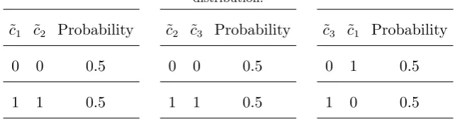
distribution. Vorob’ev (1962) provided a simple counterexample to show this for the cover E=
[image:9.595.145.466.373.462.2]{{1,2},{2,3},{1,3}} (see Table 1). In this example, there is no possible joint distribution for
Table 1 Example where consistency of the bivariate marginals does not imply feasibility of a trivariate
distribution.
˜
c1 ˜c2 Probability
0 0 0.5
1 1 0.5
˜
c2 ˜c3 Probability
0 0 0.5
1 1 0.5
˜
c3 ˜c1 Probability
0 1 0.5
1 0 0.5
(˜c1,˜c2,˜c3) even though the two-dimensional distributions of (˜c1,c2˜ ), (˜c2,˜c3) and (˜c3,˜c1) are
con-sistent on the overlapping elements. This brings us to the following definition of a regular or a
decomposable cover (see Vorob’ev (1962), Kellerer (1964)).
Definition 2. A cover structure for which the consistency of the multivariate marginals is
suffi-cient to ensure that ΘE is nonempty is referred to as a regular cover (or decomposable cover). A
cover that is not regular is referred to as an irregular cover.
While in general, there is no simple sufficient condition to test if ΘE is nonempty (see Kellerer
(1991)), for regular covers the necessary and sufficient condition is to test the pairwise consistency
2.1. Regular Cover
A regular cover is characterizable by several equivalent graph theoretic properties. We review some
of the key properties using terminology from graphs and hypergraphs (see Berge (1976)) next.
Associated with a cover is a hypergraphH(N,E) with a set of verticesN and a set of hyperedgesE
that form the set of nonempty subsets ofN. The graphG(H) associated with the hypergraphHis
a graph with the same set of vertices asHand an edge between every vertex pair that lies in some
hyperedge. Then the following four properties: (a), (b), (c) and (d) have shown to be equivalent to
each other (see Beeri et al. (1983) and Lauritzen et al. (1984)).
(a) The cover E on the setN is regular:
For a regular cover, every pairwise consistent set of multivariate marginals is also globally
consistent, namely there exists a joint distribution with the given multivariate marginals as
projections.
(b) The hypergraph H(N,E) is acyclic:
A hypergraph H is acyclic if all the vertices of Hcan be deleted by repeatedly applying the
following two operations: (1) Delete a vertex that occurs in only one hyperedge, (2) Delete
an hyperedge that is contained in another hyperedge.
(c) The hypergraph H(N,E) is conformal and chordal:
A clique of a graph G is a set of pairwise adjacent vertices. A hypergraph H is conformal if
every clique in G(H) is contained in an hyperedge of H. A graph G is chordal if every cycle
of four or more vertices has at least a chord (an edge connecting two non-adjacent vertices in
the cycle). A hypergraphH is chordal if its graphG(H) is chordal.
(d) The cover E on the setN satisfies the running intersection property (RIP):
A cover E satisfies the RIP, if the elements ofE can be ordered such that:
∀r∈ R \ {1}, ∃σr∈ R: 1≤σr< r and Jr∩
r−1
∪ t=1Jt
Associated with the RIP in (9), define the parameters:
σr, min
i∈ R
Jr∩
r−1
∪ t=1Jt
⊆ Ji
,∀r∈ R \ {1},
Kr, Jr∩
r−1
∪ t=1Jt
, ∀r∈ R \ {1}.
(10)
A feasible joint distribution can be constructed in this case using conditional independence
as follows (see Kellerer (1964) and Jirouˇsek (1991)):
θ(c) =θ1(c1)×
θ2(c2)
projK2(θ2(c2))
× · · · × θR(cR)
projKR(θR(cR))
, ∀c. (11)
Any one of the four properties: (a), (b), (c) or (d) is verifiable efficiently and in particular linear
time algorithms have been developed to test for these properties (see Rose et al. (2004) and Tarjan
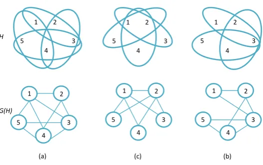
and Yannakakis (1984)). Examples of irregular and regular covers are provided in Figure 1. Covers
H
G(H)
4 3 5
1 2c
4 3 5
1 2c
4 3 5
1 2c
4 3
5
1 2
4 3
5
1 2
c
4 3
5
1 2
c
[image:11.595.168.432.425.590.2](a) (c) (b)
Figure 1 Examples of three different covers with their hypergraph and graph representations. (a) E =
{{1,2,3},{2,3,4},{3,4,5},{4,5,1}}is an irregular cover. (b)E={{1,2,3},{1,2,4},{1,2,5}}is a
regu-lar cover. (c)E={{1,2,3},{2,3,4},{3,4,5}}is a regular cover. In (a),His not acyclic. ThoughG(H) is
chordal,His not conformal since the clique{1,2,4}is not contained inE. In (b) and (c),His acyclic,
His conformal and chordal and the RIP is satisfied. In (b),σ2= 1,σ3= 1,K2={1,2},K3={1,2}. In
(b) and (c) in Figure 1 correspond to star and series covers, both of which are regular covers. A
joint distribution for the star cover in Figure 1(b) is constructed as follows:
θ(c) =θ{1,2,3}(c1, c2, c3)×
θ{1,2,4}(c1, c2, c4)
θ{1,2}(c1, c2)
×θ{1,2,5}(c1, c2, c5)
θ{1,2}(c1, c2)
, ∀c, (12)
or equivalently:
θ(c) =θ{1,2}(c1, c2)×θ{3|1,2}(c3|c1, c2)×θ{4|1,2}(c4|c1, c2)×θ{5|1,2}(c5|c1, c2), ∀c, (13)
whereθ{r|1,2}(cr|c1, c2) is the conditional distribution ofcr given c1 and c2. Similarly a joint
distri-bution for the series cover in Figure 1(c) is constructed as follows:
θ(c) =θ{1,2,3}(c1, c2, c3)×
θ{2,3,4}(c2, c3, c4)
θ{2,3}(c2, c3)
×θ{3,4,5}(c3, c4, c5)
θ{3,4}(c3, c4)
, ∀c, (14)
or equivalently:
θ(c) =θ{1}(c1)×θ{2,3|1}(c2, c3|c1)×θ{4|2,3}(c4|c2, c3)×θ{5|3,4}(c5|c3, c4), ∀c. (15)
Properties of regular covers have been previously exploited in developing efficient database
rep-resentation schemes (see Beeri et al. (1983)), in approximating high-dimensional probability
dis-tributions (see Chow and Liu (1968)), in developing tractable semidefinite relaxations in sparse
polynomial optimization problems (see Lasserre (2006)) and in developing efficient inference
algo-rithms in probabilistic graphical models (see Wainwright and Jordan (2008)). In this paper, we use
the structure of regular covers in distributionally robust optimization problems. From this point
onwards, we assume that the following condition is satisfied.
Assumption 1. The cover E is regular with the elements satisfying the RIP property in (9) and
the multivariate marginal distributions {θr}r∈R are consistent.
In Section 4, we describe a data-driven approach that uses historical return data to generate regular
covers with consistent marginal distributions. The following lemma provides a simpler condition
Lemma 1. Given a regular cover E, the following condition is necessary and sufficient to ensure
consistency among the marginal distributions:
projKr(θr) = projKr(θσr), ∀r∈ R \ {1}:Kr6=∅.
Proof. Using the RIP condition in (9), we have for all r∈ R \ {1},
Jr∩
r−1
∪ t=1Jt
⊆ Jσr ⇐⇒ Jr∩
r−1
∪ t=1Jt
⊆ Jσr∩ Jr,
⇐⇒ Jr∩ Jt⊆ Jσr∩ Jr, ∀t= 1, . . . , r−1.
This indicates that all the pairwise intersections for a regular cover are included in a set of R−
1 intersections. Thus verifying consistency can be restricted to these pairs. Since, Jσr ∩ Jr=
r−1
∪ t=1Jt
∩ Jr=Kr, the result is proved.
Lemma 1 implies that for regular covers, the feasibility of the Fr´echet class of distributions
can be ensured with O(R) consistency requirements as opposed to O(R2) pairwise consistency
requirements.
2.2. A New Fr´echet Upper Bound
In this section, we compute the upper bound ME(ϕ) for ϕ(˜c) = maxj∈M (c˜Taj+bj) for regular
covers with consistent multivariate marginals. Our main theorem provides a linear optimization
formulation to compute the Fr´echet upper bound for discrete distributions. Towards this, we define
a N-dimensional vector η that allows us to express a linear function in ˜c as separable functions
with respect to the cover E. Define theith component ofη as follows:
ηi,
1
X
r∈R
I{i∈ Jr}
, ∀i∈ N,
where I{i∈ Jr}= 1 if i∈ Jr and 0 otherwise. For example, in the simple star cover, this reduces
to:
η=
1
N−1,1, . . . ,1
T
and in the simple series cover, this reduces to:
η=
1,1
2, 1 2, . . . ,
1 2,1
T
.
Then, ˜cTa=P
r∈Rc˜
T
r (ηr◦ar) where ηr and ar are sub-vectors formed by the elements ofη and
a inJr and ◦is the Hadamard (entry-wise) product operator. Finally, let Cr denote the finite set
of support values of the sub-vectorcr˜ and Cr= size(Cr).
Theorem 1. Given a regular cover E and a consistent set {θr}r∈R of discrete marginal
distribu-tions with finite support, let MP
E(ϕ) be the optimal value to the primal linear program:
max ϑj,r(.),λj
X
j∈M
X
r∈R
X
cr∈Cr
cTr(ηr◦ajr)·ϑj,r(cr) +
X
j∈M
bjλj
s.t.(Nonnegativity of measure):
ϑj,r(cr)≥0, ∀cr∈ Cr,∀r∈ R,∀j∈ M,
(Multivariate marginal requirement):
X
j∈M
ϑj,r(cr) =θr(cr), ∀cr∈ Cr,∀r∈ R,
(Probability of jth term attaining maximum):
X
cr∈Cr
ϑj,r(cr) =λj, ∀r∈ R,∀j∈ M,
(Consistency requirement):
X
hr∈Cr:projKr(hr)=cKr
ϑj,r(hr) =
X
hσr∈Bσr:projKr(hσr)=cKr
ϑj,σr(hσr),∀cKr ∈ CKr,
∀r∈ R \ {1}:Kr6=∅,∀j∈ M,
(16)
where the decision variables are the nonnegative measuresϑj,r(cr) andλj for cr∈ Cr, r∈ R, j∈ M.
Then the Fr´echet boundME(ϕ) = maxθ∈ΘE Eθ
maxj∈M(˜c
T
aj+bj)
is equal to MP
Proof. We first show that MP
E(ϕ) is a valid upper bound of ME(ϕ). For any joint distribution
θ∈ΘE, the expected value in (2) can be expressed as follows:
Eθ[ϕ(c˜)] =Eθ
"
max j∈M
X
r∈R
˜
cTr(ηr◦ajr) +bj
!#
= X
j∈M
Eθ
" X
r∈R
˜
cTr(ηr◦ajr) +bj
thejth term is max #
Pθ(the jth term is max)
= X
j∈M
X
r∈R
X
cr∈Cr
cTr(ηr◦ajr)·Pθ(˜cr=cr, thejth term is max) +
X
j∈M
bjPθ(thejth term is max)
= X
j∈M
X
r∈R
X
cr∈Cr
cT
r(ηr◦ajr)·ϑj,r(cr) +
X
j∈M
bjλj,
where the decision variables are the measures ϑj,r(cr) and λj defined as follows:
ϑj,r(cr) =Pθ(˜cr=cr, the jth term is max),
λj =Pθ(the jth term is max).
Thus ϑj,r(cr)≥0 which corresponds to the nonnegativity of measure requirement. Note that if
the function value ϕ(c) has multiple terms attaining the maximum for some value of c, one can
arbitrarily choose any one of them without changing the expected value, for example, the term
with the minimum index. Hence, for all cr∈ Cr and r∈ R,
X
j∈M
ϑj,r(cr) =Pθ(˜cr=cr)
=θr(cr),
which corresponds to the given multivariate marginal requirement. In addition, for all r∈ R and
j∈ M,
X
cr∈Cr
ϑj,r(cr) =Pθ(the jth term is max)
=λj,
which corresponds to the probability of the jth term attaining the maximum. From Lemma 1,
consistency of the measures ϑj,r(.) for a given term j is guaranteed by equality of the projections
of the measures:
In terms of the decision variables, this corresponds to the last set of constraints in (16). Thus, for
any distribution θ∈ΘE, all the constraints in (16) are satisfied, which implies MEP(ϕ) is an upper
bound:
MEP(ϕ)≥ME(ϕ) = max
θ∈ΘE
Eθ[ϕ(c˜)].
We next prove that the bound is tight. Observe that the linear program (16) is bounded and
feasible implying that the optimal objective value is attained. Consider an optimal solution of
problem (16) denoted by ϑ∗
j,r(cr) and λ
∗
j. We have:
X
j∈M
λ∗j =
X
j∈M
X
cr∈Cr
ϑ∗j,r(cr)
= X
cr∈Cr
θr(cr)
= 1.
In addition, λ∗
j ≥0 for all j∈ M. Thus λ
∗
is a probability vector. We now construct a joint
distribution θ∗ forc˜based on ϑ∗
j,r(cr) and λ∗j as follows:
(a) Choose term j∈ Mwith probability λ∗
j.
(b) For each r∈ R, assign a measure θ∗
j,r(cr) forcr∈ Cr where θ∗j,r(cr) =ϑ∗j,r(cr)/λ∗j. Note that
ifλ∗
j= 0, we simply drop that index.
(c) Choose a feasible joint distribution in the Fr´echet class of distributionsθ∗
j∈ΘE(θj,∗1, . . . , θj,R∗ )
and generate ˜c with distributionθ∗
j.
It is clear that θ∗
j,r is a valid and consistent probability measure for cr˜, r∈ R, since (ϑ
∗
j,r(cr), λ
∗
j)
is a feasible solution to problem (16). Hence, ΘE(θ∗j,1, . . . , θ
∗
j,R)6=∅since the cover is regular, which
implies the existence of a joint distribution θ∗
j for all j∈ M. For all r∈ R, the probability of ˜cr
taking the valuecr is:
X
j∈M
λ∗j·
ϑ∗
j,r(cr)
λ∗
j
= X
j∈M
ϑ∗j,r(cr)
Thus, we haveθ∗∈Θ
E. Hence the following inequality holds:
Eθ∗j
" max k∈M X r∈R ˜
cTr(ηr◦akr) +bk
!#
≥Eθ∗j
" X
r∈R
˜
cTr(ηr◦ajr) +bj
#
=X
r∈R
Eθ∗j
˜
cTr(ηr◦ajr) +bj
=X r∈R 1 λ∗ j X
cr∈Cr
cTr(ηr◦ajr)·ϑ
∗
j,r(cr) +bj,
where the first inequality is obtained by simply choosing thejth term in the function forθ∗j. Then
we have a lower bound since:
Eθ∗
" max k∈M X r∈R ˜
cTr(ηr◦akr) +bk
!#
= X
j∈M
λ∗j·Eθj∗
" max k∈M X r∈R ˜
cTr(ηr◦akr) +bk
!#
≥ X
j∈M
λ∗j
" X r∈R 1 λ∗ j X
cr∈Cr
cTr(ηr◦ajr)·ϑ
∗
j,r(cr) +bj
# = X j∈M X r∈R X
cr∈Cr
cT
r(ηr◦ajr)·ϑ
∗
j,r(cr) +bjλ∗j
=MEP(ϕ).
Hence
ME(ϕ) = max
θ∈ΘE E
θ max j∈M aT j˜c+bj
≥Eθ∗
max j∈M
aT j˜c+bj
≥MP
E (ϕ).
Together, we have ME(ϕ) =MEP(ϕ).
Several remarks about the theorem and its proof are in order:
(a) The proof of Theorem 1 is inspired from the proofs in Bertsimas et al. (2006) and
Natara-jan et al. (2009b) for univariate marginals and Doan and NataraNatara-jan (2012) for
non-overlapping multivariate marginals. Theorem 1 extends these results to non-overlapping
multivari-ate marginals. The main generalization is that we incorpormultivari-ate a new set of linear constraints
that guarantee the consistency of the distributions and thereby the existence of a joint
dis-tribution that attains the bound for overlapping regular covers.
(b) The conditionally independent distribution in (11) is a feasible distribution in the set ΘE. This
(1991)). Theorem 1 provides an alternate distribution in the set ΘE that maximizes the
expected value of a piecewise linear convex function of the random vector.
(c) The representation of the split vector η is not unique. In particular, we can define values
ηr
i ≥0, such that
P
r∈Rη
r
i = 1 and η r
i = 0 if i6∈ Jr for all r∈ R and i∈ N. For example,
instead of splitting variables equally among all the relevant subsets, we can set ηir(i)= 1 for
all i∈ N, where r(i) = min{r:i∈ Jr}. This does not affect the result of Theorem 1.
(d) A total of P
r∈RCr probabilities are specified as an input to the linear optimization problem
where Cr is the support of each sub-vector cr˜. The total number of decision variables in the
primal linear program in Theorem 1 isMP
r∈RCr+M, and the total number of constraints
is MP
r∈RCr+RM+
P
r∈RCr+M
P
r∈R\{1}CKr. Hence the size of the linear program is
polynomially bounded in the parametersN,M,Rand the maximum support size maxr∈RCr.
If the marginals are constructed from historical data, as in the numerical experiments in
Section 4, the maximum support size is bounded by the number of data samples. With the
number of data samples in the order of hundred, we will demonstrate in the numerical section
that the linear program (16) can be solved efficiently.
(e) It is possible for the maximum support size maxr∈RCr to be exponential in the number of
random variablesN. For example, if the entire joint distribution is given, up toKN
probabili-ties might need to be specified whereKis the maximum number of values that any individual
random variable takes. In this case, if the size of the subsets are restricted to be O(log(N)),
then maxr∈RCr≤KO(log(N)) and is polynomially bounded in N. The size of the linear
pro-gram is then polynomially bounded in the parametersN,M,RandK (the maximum number
of support points of any univariate marginal). In general, if the size of the subsets is small
enough as compared toN, solving the linear program (16) to compute Fr´echet bounds would
be more efficient than computing the expected value (2) given the complete joint distribution
of up to KN probabilities.
We conclude this section by showing that the result in Doan and Natarajan (2012) for general
variablesfr(cr),dj,r and gj,r(cKr) to the equalities in formulation (16), the dual linear program is
formulated as follows:
MED(ϕ) = min
fr(·),gj,r(·),dj,r
X
r∈R
X
cr∈Cr
fr(cr)θr(cr)
s.t. fr(cr)≥cTr(ηr◦ajr)−dj,r−gj,r(cKr) +
X
t>r:σt=r
gj,t(cKt),∀cr∈ Cr,
∀r∈ R,∀j∈ M,
X
r∈R
dj,r+bj= 0, ∀j∈ M,
(17)
where we defineK1=∅, and for r∈ R, ifKr=∅, we define c˜Kr= 0, and gj,r(0) = 0, for all j∈ M.
Formulation (17) can be concisely rewritten as:
MED(ϕ) = min gj,r(·),dj,r
X
r∈R
Eθr
"
max
j∈M ˜c
T
r(ηr◦ajr)−dj,r−gj,r(c˜Kr) +
X
t>r:σt=r
gj,t(˜cKt)
!#
s.t.X
r∈R
dj,r+bj= 0, ∀j∈ M,
(18)
Linear programming duality implies thatME(ϕ) =MED(ϕ). For a general partition, the dual
vari-ables gj,r(cKr) correspond to the marginal consistency constraints in the primal problem (16).
When E is a partition, the marginal consistency constraints are not present and hence the
corre-sponding dual variables are deleted. Thus formulation (17) for the partition case reduces to:
min dj,r
X
r∈R
Eθr
max j∈M c˜
T
rajr−dj,r
s.t.X
r∈R
dj,r+bj= 0, ∀j∈ M,
(19)
which is equivalent to the non-overlapping marginal formulation in Doan and Natarajan (2012).
2.3. Connected Regular Covers: Star and Series Case
In this section, we simplify the Fr´echet bound for a class of covers with a special structure that we
term asconnected regular covers.
Definition 3. A coverE is said to be connected if for anys, t∈ R,s6=t, there exists a sequence
It is clear that partitions are not connected covers. The simple star and series covers are examples
of connected covers. The next lemma characterizes the connectedness of regular covers.
Lemma 2. A regular cover E is connected if and only ifKr6=∅ for all r∈ R \ {1}.
The proof of the Lemma is provided in the Appendix. This characterization of connected regular
covers allows us to slightly simplify the formulation to compute ME(ϕ).
Proposition 1. Given a connected regular cover E and a consistent set {θr}r∈R of discrete
marginal distributions with finite support, let MPC
E (ϕ) be the optimal value to the primal linear
program:
max ϑj,r(.)
X
j∈M
X
r∈R
X
cr∈Cr
cT
r(ηr◦ajr) +ρrbj
·ϑj,r(cr)
s.t.(Nonnegativity of measure):
ϑj,r(cr)≥0, ∀cr∈ Cr,∀r∈ R,∀j∈ M,
(Multivariate marginal requirement):
X
j∈M
ϑj,r(cr) =θr(cr), ∀cr∈ Cr,∀r∈ R,
(Consistency requirement):
X
hr∈Cr: projKr(hr)=cKr
ϑj,r(hr) =
X
hσr∈Cσr: projKr(hσr)=cKr
ϑj,σr(hσr),∀cKr∈ CKr,
∀r∈ R \ {1},∀j∈ M,
(20)
where ρr are arbitrary constants that satisfy
P
r∈Rρr = 1 and the decision variables
are the measures ϑj,r(cr) for cr ∈ Cr, r ∈ R, j ∈ M. Then the Fr´echet bound ME(ϕ) =
maxθ∈ΘE Eθ
maxj∈M (c˜
T
aj+bj)
is equal to MPC
E (ϕ).
Proof. We claim that the constraints:
X
cr∈Cr
ϑj,r(cr) =λj, ∀r∈ R,∀j∈ M,
in (16) are redundant if the regular cover E is connected. From Lemma 2, Kr6=∅ for all r∈ R.
Using the last set of constraints in (16) (or (20)), we obtain the following equalities:
X
cr∈Cr
ϑj,r(cr) =
X
cs∈Cs
Thus, we can drop the decision variables λj, by replacing
P
j∈Mbjλj by
P
j∈M
P
r∈R
P
cr∈Crρrbjϑj,r(cr) in the objective given that
P
r∈Rρr = 1. Thus for connected
regular covers, (20) is equivalent to (16) and it implies that in this case, ME(ϕ) =MEPC(ϕ).
The problem (20) has fewer variables and lesser constraints as compared to (16), which also
allows us to simplify its dual formulation by remove the corresponding set of dual variables. The
dual formulation is written as follows:
MEDC(ϕ) = min
gj,r(·)
X
r∈R
Eθr
"
max
j∈M ˜c
T
r(ηr◦ajr)−gj,r(c˜Kr) +
X
t>r:σt=r
gj,t(˜cKt) +ρrbj
!#
. (21)
To illustrate this formulation, we consider two simple examples of the Fr´echet bound for star and
series covers.
Series cover:For the simple series cover, we haveR=N−1 andσr=r−1 for allr= 2, ..., N−1.
Letting ρr= 1/(N−1) for allr∈ R, we can reformulate (21) as:
min gj,r(.)
Eθ{1,2}
max j∈M
˜
c1aj1+ ˜
c2aj2
2 +gj,2(˜c2) +
bj
N−1
+
N−2
X
r=2
Eθ{r,r+1}
max j∈M
˜
craj r
2 +
˜
cr+1aj r+1
2 −gj,r(˜cr) +gj,r+1(˜cr+1) +
bj
N−1
+
Eθ{N−1,N}
max j∈M
˜
cNaj N+ ˜
cN−1aj N−1
2 −gj,N−1(˜cN−1) +
bj
N−1
.
(22)
Star cover:For the simple star cover, we have R=N−1 andσr= 1 for all r= 2, . . . , N−1. The
dual Fr´echet bound for the star cover is reformulated from (21) as follows:
min gj,r(.)
Eθ{1,2}
"
max
j∈M c2a˜ j2+ ˜c1aj1+
N−1
X
r=2
gj,r(˜c1) +bj
!#
+ N−1
X
r=2
Eθ{1,r+1}
max
j∈M ˜cr+1aj r+1−gj,r(˜c1)
.
We define a new set of decision variables as follows:
gj,1(c1) =−
N−1
X
r=2
gj,r(c1)−c1aj1−bj, ∀c1∈ C1,∀j∈ M.
The formulation then reduces to:
min gj,r(.)
N−1
X
r=1
Eθ{1,r+1}
max
j∈M ˜cr+1aj r+1−gj,r(˜c1)
s.t.
N−1
X
r=1
gj,r(c1) =−c1aj1−bj, ∀c1∈ C1,∀j∈ M.
Conditioning with respect to the marginal distribution of ˜c1 as in Puccetti and R¨uschendorf (2012)
and using the dual representation for the partition case in (19), we obtain an equivalent formulation:
Eθ{1}
(
sup
θ∈Θ{{2|1},...,{N|1}}E
θ
max j∈M c˜
T aj+bj
˜c1
)
.
For a fixed ˜c1=c1, the inner problem is the Fr´echet bound where θ belongs to the Fr´echet class
defined by the conditional marginal distributions. Thus, the Fr´echet bound for the star cover is
equivalent to:
Eθ{1}
(
sup θ∈Θ{{2|1},...,{N|1}}
Eθ
h
ϕ(˜c)
c1˜ i ) ,
which indicates that it is reduces to the computation of Fr´echet bounds with a simple partition. A
similar observation has been made by Puccetti and R¨uschendorf (2012) for more general objective
functions.
3. Bounds for CVaR and VaR
In this section, we evaluate new Fr´echet bounds for the CVaR and VaR measures.
3.1. CVaR Bound
The worst case CVaR with respect to the Fr´echet class of distributions for α∈(0,1) is defined as
(see Natarajan et al. (2009a) and Zhu and Fukushima (2009)):
WCVaRΘE
α c˜
T
x
, sup θ∈ΘE
CVaRθα ˜cTx
= sup θ∈ΘE
min β∈<
β+ 1 1−αEθ
h
˜
cTx−β+
i
.
(24)
Since the multivariate marginal distributions{θr}r∈Rare assumed to be discrete with finite support,
the expected value is finite and the supremum is attained by a joint distribution. Interchanging
the minimum and maximum in the worst-case CVaR formulation and from the convexity of the
objective function with respect toβ and linearity with respect to the measureθ, we get:
WCVaRΘE
α c˜
T
x
= min β∈<
β+ 1
1−αmaxθ∈ΘEEθ
h
˜
cTx−β+i
. (25)
Thus, in order to compute the upper bound on the CVaR, we need to compute an upper bound on
the expected value Eθ
h
˜
cTx−β+i
. We provide a simple example to illustrate the computation
3.1.1. Example Consider a sum of N random variables. We compute the Fr´echet upper
bound:
max θ∈ΘE
Eθ
X
i∈N
˜
ci−β
!+
(26)
and compare it with expected value under the maximum entropy (ME) distribution in (11):
EME
X
i∈N
˜
ci−β
!+
.
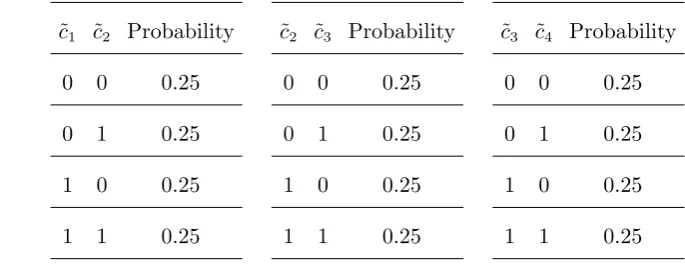
Consider the bivariate uniform discrete distributions provided in Table 2 for a simple series cover
withN= 4. The maximum-entropy distribution in this case is the independent uniform distribution
[image:23.595.122.465.594.729.2]withPME(c) = 1/16 for all c∈ {0,1}4.
Table 2 Consistent bivariate marginals for simple series cover withE={{1,2},{2,3},{3,4}}.
˜
c1 ˜c2 Probability
0 0 0.25
0 1 0.25
1 0 0.25
1 1 0.25
˜
c2 ˜c3 Probability
0 0 0.25
0 1 0.25
1 0 0.25
1 1 0.25
˜
c3 ˜c4 Probability
0 0 0.25
0 1 0.25
1 0 0.25
In order to compute the upper bound, we apply Proposition 1 with M = 2, a1=e, b1=−β,
a2=0 and b2= 0. The primal linear program for (26) is formulated as follows:
max ϑr(·)
X
(v,w)∈{0,1}2
v+w 2 −
β
3
·ϑ{1,2}(v, w) +
v 2+ w 2 − β 3
·ϑ{2,3}(v, w)
+
X
(v,w)∈{0,1}2
v
2+w−
β
3
·ϑ{3,4}(v, w)
s.t.(Nonnegativity of measure):
ϑ{1,2}(v, w), ϑ{2,3}(v, w), ϑ{3,4}(v, w)≥0, ∀(v, w)∈ {0,1}2,
(Multivariate marginal requirement):
ϑ{1,2}(v, w)≤0.25, ∀(v, w)∈ {0,1}2,
ϑ{2,3}(v, w)≤0.25, ∀(v, w)∈ {0,1}2,
ϑ{3,4}(v, w)≤0.25, ∀(v, w)∈ {0,1}2,
(Consistency requirement):
ϑ{2,3}(0,0) +ϑ{2,3}(0,1) =ϑ{1,2}(0,0) +ϑ{1,2}(1,0),
ϑ{2,3}(1,0) +ϑ{2,3}(1,1) =ϑ{1,2}(0,1) +ϑ{1,2}(1,1),
ϑ{3,4}(0,0) +ϑ{3,4}(0,1) =ϑ{2,3}(0,0) +ϑ{2,3}(1,0),
ϑ{3,4}(1,0) +ϑ{3,4}(1,1) =ϑ{2,3}(0,1) +ϑ{2,3}(1,1),
(27)
Since the support of P
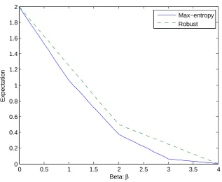
i∈Nc˜i is restricted in {0,1,2,3,4}, we vary β in [0,4]. Figure 2 provides
a comparison of the bounds. The Fr´echet bound provides an upper bound on the expected value
with respect to the maximum-entropy distribution.
We next incorporate the bound to provide an explicit formulation for the Fr´echet bound of
CVaR. Applying the dual formulation, the worst-case CVaR bound is computed as follows:
WCVaRΘE
α X i∈N ˜ ci ! = min gr(.),β
β+
1 1−α
X
r∈R
Eθr
c˜
T
rηr−gr(˜cKr) +
X
t>r:σt=r
gt(c˜Kt)−
0 0.5 1 1.5 2 2.5 3 3.5 4 0
0.2 0.4 0.6 0.8 1 1.2 1.4 1.6 1.8 2
Beta: β
Expectation
[image:25.595.145.463.74.334.2]Max−entropy Robust
Figure 2 Comparison between the Fr´echet bound and the maximum entropy distribution
For the distributional information in Table 2, we can reformulate (28) with additional decision
variables as a linear program:
min gr(.),β,zr(.)
β+ 1 4(1−α)
X
(v,w)∈{0,1}2
z{1,2}(v, w) +z{2,3}(v, w) +z{3,4}(v, w)
s.t. z{1,2}(v, w)−g{2,3}(w)≥v+
w
2 −
β
3, ∀(v, w)∈ {0,1}
2,
z{2,3}(v, w) +g{2,3}(v)−g{3,4}(w)≥
v
2+
w
2 −
β
3, ∀(v, w)∈ {0,1}
2,
z{3,4}(v, w) +g{3,4}(v)≥
v
2+w−
β
3, ∀(v, w)∈ {0,1}
2,
z{1,2}(v, w), z{2,3}(v, w), z{3,4}(v, w)≥0, ∀(v, w)∈ {0,1}2.
(29)
3.2. VaR Bound
The VaR for a portfolio forα∈(0,1) is defined as:
VaRθα ˜cTx
,inf
z∈ <:Pθ c˜ T
x≤z
≥α .
Hence, we have the following equivalence:
VaRθα ˜c T
x≤z ⇔ Pθ ˜c
T
which implies that z is an upper bound of VaRθα c˜Tx
, if and only if α is a lower bound of the
cumulative distribution function Pθ ˜c T
x≤z. Since CVaR dominates VaR (see Rockafellar and
Uryasev (2002)), we can use CVaR to derive lower bounds of the cumulative distribution function
value. Given a Fr´echet class ΘE of distributions, the worst-case VaR is defined as follows:
WVaRΘE
α (c˜ T
x) ,inf
z∈ <: inf θ∈ΘEP
θ c˜ T
x≤z≥α
. (30)
Since WVaRΘE
α (˜c T
x) = sup θ∈ΘE
VaRθα(x), this implies WVaR
ΘE
α (c˜ T
x)≤WCVaRΘE
α (c˜ T
x).
3.2.1. Example In the following example, we provide a lower bound on the cumulative
dis-tribution function of the sum of random variables Pθ
P
i∈N˜ci≤z
using CVaR approximations.
Observe that,
WVaRΘE
α X i∈N ˜ ci !
≤z ⇔ inf
θ∈ΘEP
θ
X
i∈N
˜
ci≤z
!
≥α,
The Fr´echet bounds are related as follows:
inf θ∈ΘEP
θ
X
i∈N
˜
ci< z
!
≤ inf
θ∈ΘEP
θ
X
i∈N
˜
ci≤z
!
≤ inf
θ∈ΘEP
θ
X
i∈N
˜
ci≤z+
!
for all >0.
Since WCVaR is an upper bound on WVaR, we first compute the WCVaR bound and then use
numerical inversion to find a lower bound on the cumulative distribution function. For the series
cover, we compute the worst-case CVaR as follows:
WCVaRΘE
α X i∈N ˜ ci ! = min gi(.),β
β+ 1
1−α Eθ{1,2}
"
˜
c1+c2˜
2 +g2(˜c2)−
β N−1
+#
+
N−2
X
i=2
Eθ{i,i+1}
"
˜
ci+ ˜ci+1
2 −gi(˜ci) +gi+1(˜ci+1)−
β N−1
+#
+
Eθ{N−1,N}
"
˜
cN−1
2 + ˜cN −gN−1(˜cN−1)−
β N−1
+#!
.
(31)
For the numerical experiment, we construct bivariate marginal distributions for the simple series
cover by using the independent copula and identical uniform univariate marginals in [0,1]. Then
Fi(ci) =cifor allci∈[0,1] and the joint distribution for two random variables is isFi,i+1(ci, ci+1) =
cici+1 for all (ci, ci+1)∈[0,1]2 withi= 1, . . . , N−1. Clearly the set of these bivariate marginals is
optimization problem. To compute WCVaR, we use a discretization of the distribution function
to compute upper and lower bounds. Consider a discrete distribution ˆFω approximation ofF with
M-points as in Embrechts and Puccetti (2010):
ˆ
Fω, 1
M
X
j∈M
I{x≥ωj},
where ω={ω1, ..., ωM} is the set of M jump points. Let qj=
j
M for j= 0, . . . , M and define two
sets of jump pointsω={q1, . . . , qM}andω={q0, . . . , qM−1}. Clearly, ˆFω and ˆFω provide lower and
upper bounds forF. The discretized bivariate marginal distributions are constructed from the
cor-responding discretized univariate marginals using the independent copula. Let WCVaRΘαE(
P
i∈N˜ci)
and WCVaRΘE
α (
P
i∈Nc˜i) denote the worst case CVaR bounds with respect to the discretized
marginals respectively. Then, WCVaRΘE
α (
P
i∈N˜ci)≤WCVaR
ΘE
α
P
i∈Nc˜i
≤WCVaRΘαE(P
i∈N˜ci).
The upper and lower bounds are computed from the linear optimization problem in (31).
Embrechts and Puccetti (2010) proposed a lower bound of the cumulative distribution function
of the sum of random variables using the standard bound in (8) with variable splitting. In order
to compute this bound, one needs to calculate Fy(d) =P ˜c1+
˜
c2 2 ≤d
and Fz(d) =P
˜
c1 2 +
˜
c2 2 ≤d
.
In our example, this reduces to:
Fy(d) =
0, d <0,
d2, 0≤d <1/2,
d−1/4, 1/2≤d <1,
−d2+ 3d−5/4,1≤d <3/2,
1, d≥3/2,
and Fz(d) =
0, d <0,
2d2, 0≤d <1/2,
−2d2+ 4d−1,1/2≤d <1,
1, d≥1.
Note that F−
y (d) =Fy(d) and Fz−(d) =Fz(d) given continuous distributions. The lower bound in
Embrechts and Puccetti (2010) (referred to as thereduced standard bound (RSB)) is computed as
follows:
RSB(x) = max
(
sup d∈<N−2
"
Fy(d1) +Fy x− N−2
X
i=1 di
!
+ N−2
X
i=2 Fz(di)
#
−(N−2),0
)
The objective function in the inner maximization problem in (32) is unfortunately not concave,
making it challenging to find optimal solutions for the optimization problem. To solve this problem,
we use a numerical procedure outlined in the Appendix. In our computations, we set M= 50 and
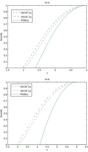
compute the newseries CVaR based bounds (SECB). The two bounds on the cumulative
distribu-tion funcdistribu-tion SECB+(x) and SECB−(x) are evaluated by taking the inverse of WCVaRΘαE(
P
i∈N˜ci)
and WCVaRΘE
α (
P
i∈Nc˜i), respectively. Figure 3 shows the three bounds, RSB(x), SECB
+
(x), and
SECB−(x), for N= 4 and N = 6. Observe that SECB+(x) and SECB−(x) are fairly close to each
other. Since the actual CVaR bound lies the between the two curves, the discrete approximation
withM= 50 for CVaR bounds is reasonably good in this example. It is also clear that our proposed
approximation significantly improves on the existing reduced standard bound.
4. Robust Portfolio Optimization
In this section, we implement the distributionally robust portfolio optimization approach in two
financial datasets and compare it with the sample based approach. Consider a portfolio of N
assets and let ξ˜be the random return vector of the assets. The random loss of ith asset is then
simply ˜ci=−ξ˜i. Given a feasible asset allocation x∈ X, the computation of CVaR of the joint
portfolio requires the distribution of the random return vector c˜. Assume that we have access to
historical data of a finite set of samples from the financial market denoted by the setC. The sample
distribution θ assigns a probability of 1/C to each sample vector in C. The optimal sample-based
allocation with the minimum CVaR is obtained by solving:
min
β∈<,x∈X β+
1 (1−α)C
X
c∈C
h
cTx−β+
i !
, (33)
which is representable as a linear program. However, the out of sample performance of such a
approach is not necessarily good due to the possibility that the out of sample distribution is different
from the in-sample distribution. Using simulated data, Lim et al. (2011) have shown that the CVaR
measure with sample-based optimization results in fragile portfolios that are often unreliable due
1.5 2 2.5 3 3.5 4 0
0.1 0.2 0.3 0.4 0.5 0.6 0.7 0.8 0.9 1
x
bounds
N=4
SECB+(x) SECB−(x) RSB(x)
2.5 3 3.5 4 4.5 5 5.5 6 6.5 0
0.1 0.2 0.3 0.4 0.5 0.6 0.7 0.8 0.9 1
x
bounds
N=6
[image:29.595.160.443.79.566.2]SECB+(x) SECB−(x) RSB(x)
Figure 3 Different bounds of the cumulative distribution function of the sum of random variables with the simple
series cover
stable dependencies among the random losses and only incorporate this reliable information into
solve the following distributional robust optimization problem:
min x∈Xθmax∈ΘE
CVaRθα(˜c T
x). (34)
Using the dual representation in (28), the distributional robust portfolio optimization problem is
formulated as:
min gr(.),β,x
β+
1 1−α
X
r∈R
Eθr
c˜
T
r(ηr◦xr)−gr(c˜Kr) +
X
t>r:σt=r
gt(˜cKt)−
β R
!+
s.t. x∈ X.
(35)
IfX is a polyhedron and the multivariate marginal support set ofcr˜ isCr with each sub-vector in
the set equally likely, problem (35) is solvable as a linear optimization problem:
min gr(.),β,x,zr(.)
β+ 1 1−α
X
r∈R
X
cr∈Cr
zr(cr)
Cr
s.t. zr(cr) +gr(cKr)−
X
t>r:σt=r
gt(cKt)≥c
T
r(ηr◦xr)−
β
R,∀cr∈ Cr,∀r∈ R,
zr(cr)≥0, ∀cr∈ Cr,∀r∈ R,
x∈ X.
(36)
Next, we discuss a data-driven approach to construct the Fr´echet class of distributions of asset
returns ΘE.
4.1. Construction of Regular Covers
In the context of distributionally robust optimization, the dependency structure of the random
variables is often incorporated using moment information. Some of the common classes of
dis-tributions employed in the financial literature are disdis-tributions with first and second moment
information (see for example, El Ghaoui et al. (2003), Natarajan et al. (2009a), and Delage and Ye
(2010)) and multivariate normal distributions with parameter uncertainty in the mean and
covari-ance matrix (see Garlappi et al. (2007)). The resulting optimization formulations are tractable
conic programs. Our approach is to use a Fr´echet class of distributions with possibly overlapping
aspect of such an approach is to identify the cover structureE to balance over-fitting the data and
getting overly conservative solutions due to lack of information. In order to construct the coverE,
we use time-dependent correlation information of the asset returns.
Our underlying assumption in identifying the cover is that we include pairs of assets in the same
subset if the changes in correlation between the two assets over time is minimal. We propose the
following two step data-driven approach to identify the regular cover:
Step 1: Split the historical data into two sets of equal size and construct the sampling
dis-tributions P1 and P2 for the asset returns from these two sets. For each pair of assets (i, j), we
compute ∆ρi,j=|ρPi,j1−ρP
2
i,j|, where ρQi,j is the correlation of the losses of two assetsi and j for the
distribution Q. The simplest choice of correlation is the common Pearson correlation coefficient
but other correlation measures could also be chosen. The objective is to identify the pairs (i, j)
of assets with small values of ∆ρi,j. Under the assumption that the stable dependency structure
is captured by pairs with minimal change in correlation over time, these pairs of assets should be
included in the same subset. There are different ways to identify such pairs of assets. In this paper,
we implement two such approaches:
(a) Minimum spanning tree approach (MST):Use ∆ρi,j as the weight for the edge (i, j)
in a complete graph ofN vertices. Find the minimum spanning tree in this graph and keep allN−1
pairs of assets which define the tree. The choice of the minimum spanning tree implies that pairs
with small changes in correlation coefficients over time are likely to be selected. The MST approach
is inspired from the Chow-Liu method (Chow and Liu (1968)) which provides a second-order
product approximation of a joint probability distribution using the mutual information measure
and the spanning tree algorithm. We employ a similar method but use changes in the correlation
coefficients as the cost terms.
(b) Edge budgeting based approach (EB): Remove all the pairs except for a fraction
ra ∈[0,1] of the total number of N(N−1)/2 pairs with the smallest values of ∆ρi,j. Clearly, if
ra= 0, no pair will be selected. On the other hand, ifra= 1, we keep all the pairs. The parameter
Step 2:Construct an undirected graphGwhere the set of nodes is the set of assets, and the set
of edges is the pairs of assets selected in Step 1. If the graph G is chordal then one can construct
a regular coverE efficiently. A linear time lexicographic breadth-first search (L-BFS) algorithm is
used to determine whether a graph is chordal and to construct the regular coverE (see Rose et al.
(2004) and Tarjan and Yannakakis (1984)).
For MST approach, the graph is a tree and hence chordal. The resulting cover E has N −1
two-element subsets corresponding to individual selected pairs. The MST cover can be viewed as a
generalization of the simple star and simple series covers. In general, the resulting graph from EB
approach is not chordal. If the graphG is not chordal, one adds in a set of additional edges, which
are called fill-in edges, to make the graph chordal. Even though the problem of finding the fill-in
with the minimum number of edges is NP-complete (see Yannakakis (1981)), there are efficient
algorithms to find fill-ins with reasonably small number of edges (see for example, Huang and
Dar-wiche (1996) and Natanzon et al. (2000)). In our experiments, we use theminweightElimOrder
function in PMTK3, a Matlab toolkit for probabilistic modeling (see Dunham and Murphy (2012)),
which is based on a fill-in algorithm developed by Huang and Darwiche (1996). One can then
construct a regular coverEfrom the modified chordal graph using the L-BFS algorithm. Note that
this data-driven approach of identifying regular covers is only heuristic. When we use fill-in edges,
there will pairs of assets with larger change in correlation over time included in the cover. We will
show in Section 4 some examples of how many fill-in edges are needed for the regular covers and
how changes in correlation over time of these additional pairs of assets are compared with those of
original ones.
Given a regular cover E, the marginals are constructed from historical data. Financial data is
however non-stationary. While one could use the original sampling marginals if sufficient stationary
historical data is available, in our experiments we found that it was difficult to get a nontrivial
Fr´echet class of distribution with the data of a few hundred days. To tackle this issue, we round
is to cluster the historical data of each asset return into several clusters and to replace the data
within each cluster by the respective cluster mean. The marginals with the rounded samples are
then used in the optimization approach. Under this construction, the mean of the rounded samples
remains the same as that of original ones. Another benefit is that the size of supports of marginal
distributions is reduced and this reduces the computational time to solve the problems. In the
next section, we investigate the effects of the rounding procedure as well as the effects of using
dependence structures in numerical experiments with real financial market data.
4.2. Dataset 1: Fama-French Portfolio
Given the volatility of financial markets, investors re-balance their portfolios periodically. We solve
the portfolio optimization problem in each period under the assumption that historical daily return
data of assets from the last two periods are available and are used to estimate distributions of daily
returns in the current period. We allow for short selling and consider the following set of allowable
allocations:
X=
x∈ <n:eTx= 1,µTx≥µ
t ,
where e is the vector of all ones, µt is the target return and µ is the expected return vector of
all assets. Given the Fr´echet class of distributions obtained either from the MST or EB approach,
we solve (36) to find the portfolio allocation in each period. In order to evaluate results obtained
from the distributionally robust optimization approach, we compare the results with two other
approaches:
1. Sample-based approach (SB):The original sample distribution is used and the allocation
is computed by solving the problem (33).
2. Rounded-sampled-based approach (RSB): The rounded sample distribution is used in
(33) instead of the original sample distribution. This strategy serves as a control to validate that
the effect of the rounding procedure is not drastic.
The first data set we analyze consists of historical daily returns of an industry portfolio obtained
AMEX and NASDAQ stocks classified by industry. This include industries such as finance, health,
textiles, food and machinery. A total of 4400 observations of daily return data were available in
a period spanning approximately 15 years before the financial crisis, from August 18, 1989 to
February 1, 2007. Consider an investor who plans to invest in the portfolio with N = 49 risky
assets. He would like to minimize the risk of his investment, while guaranteeing a certain level of
average return by choosing an appropriate trading strategy. The investor re-balances his portfolio
every 200 days. We divide the 4400 samples into 22 periods, with each period consisting of 200
days. The investor starts his investment from the beginning of the third period. From then on, at
the beginning of each period, the investor uses the portfolio return data of the last two periods to
make the decision on the portfolio allocation for the current period.
In the experiments, we cluster the return data into 10 clusters. We use the R package
Ckmeans.1d.1p, which is based on ak-means clustering dynamic programming algorithm in one
dimension (see Wang and Song (2011)). The target returnµt is varied between 0.04% and 0.08%.
For each target return, we apply the four trading strategies for 20 periods. We then compute the
aggregate out of sample mean and out of sample CVaR. The out of sample efficient frontier is
constructed by varying the target return. The numerical tests were conducted in 64-bit Matlab
2011a with the CVX solver (see CVX Research Inc. (2012)).
1.55 1.6 1.65 1.7 1.75 1.8 1.85 1.9 1.95 2 0.02
0.025 0.03 0.035 0.04 0.045 0.05 0.055 0.06
out of sample cvar
out of sample mean
EB approach with different ra
ra=0 ra=0.05 ra=0.1 ra=0.15 ra=0.2 ra=0.3 ra=0.65 ra=1
1.6 1.65 1.7 1.75 1.8 1.85 1.9 1.95 0.02
0.025 0.03 0.035 0.04 0.045 0.05 0.055 0.06
out of sample cvar
out of sample mean
Different strategies
SB RSB MST EB r
[image:34.595.97.513.531.696.2]a=0.15
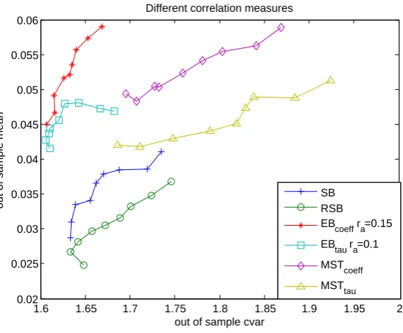
The graph on the left in Figure 4 shows the out of sample efficient frontiers of the EB trading
strategy for different values of the parameterra whenα= 0.95. Ifra= 0, the EB strategy uses only
univariate marginals and in this example, its efficient frontier is worse than that of the EB strategy
for other small values ofra. This is to be expected since we use no dependency information from the
financial market in this case. Asra increases, the performance of the EB strategy improves, and the
best efficient frontier is achieved aroundra= 0.15. The performance then gradually deteriorates as
racontinues to increase to 1. This result indicates that by using only partial dependency information
it is possible to enhance the performance of the trading strategy in the out of sample data. The
graph on the right in Figure 4 shows the efficient frontiers of the four different strategies. The
EB strategy is plotted for the optimum value ra= 0.15. We can see that optimal EB and MST
strategies are the better performing strategies in comparison to SB and RSB.
A well-known phenomenon in financial data is that the estimation of the out of sample mean is
inaccurate (see Merton (1980)). The out of sample means are between 0.03% and 0.055%, while
the target returns are between 0.04% and 0.08%. We conduct an experiment directly using the
out of sample mean data in the optimization formulation. While clearly impractical, this serves
to check the effect of the inaccuracies in the estimation of the mean return on the comparative
performance of the different strategies. Figure 5 shows that in this case the EB strategy is the best
performing strategy while the MST strategy does not perform as well. From these experiments, we
conclude that the optimal EB strategy achieves the best performance in this dataset. Note that our
approach is completely data-driven from identifying the cover to computing the optimal portfolio.
4.2.1. Robustness Tests In this section, we test the robustness of the results, by
implement-ing the distributional robust optimization model with a few modifications.
1. In the first test, we vary the CVaR parameter α. The results with α= 0.9 are displayed
in Figure 6. The best EB strategy is obtained around ra = 0.1. Similar to the results obtained
withα= 0.95, the performance of EB and MST are better than sample-based approaches and the