Dynamic covariance models

(1)

Original citation:

Chen, Ziqi and Leng, Chenlei. (2015) Dynamic covariance models. Journal of the American Statistical Association.http://dx.doi.org/10.1080/01621459.2015.1077712

Permanent WRAP url:

http://wrap.warwick.ac.uk/72728

Copyright and reuse:

The Warwick Research Archive Portal (WRAP) makes this work of researchers of the University of Warwick available open access under the following conditions. Copyright © and all moral rights to the version of the paper presented here belong to the individual author(s) and/or other copyright owners. To the extent reasonable and practicable the material made available in WRAP has been checked for eligibility before being made available.

Copies of full items can be used for personal research or study, educational, or not-for-profit purposes without prior permission or charge. Provided that the authors, title and full bibliographic details are credited, a hyperlink and/or URL is given for the original metadata page and the content is not changed in any way.

Publisher statement:

"This is an Accepted Manuscript of an article published by Taylor & Francis Group in Journal of the American Statistical Association on 7/08/2015, available online:

http://www.tandfonline.com/10.1080/01621459.2015.1077712

.A note on versions:

The version presented here may differ from the published version or, version of record, if you wish to cite this item you are advised to consult the publisher’s version. Please see the ‘permanent WRAP url’ above for details on accessing the published version and note that access may require a subscription.

(2)

Dynamic Covariance Models

∗

Ziqi Chen

†

and Chenlei Leng

‡

Abstract

An important problem in contemporary statistics is to understand the relationship

among a large number of variables based on a dataset, usually with p, the number of

the variables, much larger thann, the sample size. Recent efforts have focused on modeling

static covariance matrices where pairwise covariances are considered invariant. In many

real systems, however, these pairwise relations often change. To characterize the changing

correlations in a high dimensional system, we study a class of dynamic covariance models

(DCMs) assumed to be sparse, and investigate for the first time a unified theory for

un-derstanding their non-asymptotic error rates and model selection properties. In particular,

in the challenging high dimension regime, we highlight a new uniform consistency theory

in which the sample size can be seen as n4/5 when the bandwidth parameter is chosen as

h∝n−1/5for accounting for the dynamics. We show that this result holds uniformly over a

range of the variable used for modeling the dynamics. The convergence rate bears the mark

of the familiar bias-variance trade-off in the kernel smoothing literature. We illustrate the

results with simulations and the analysis of a neuroimaging dataset.

Key Words: Covariance model; Dynamic covariance; Functional connectivity; High

Dimen-sionality; Marginal independence; Rate of convergence; Sparsity; Uniform consistency.

∗_{We thank the Joint Editor, an Associate Editor and two reviewers for their constructive comments. We also}

acknowledge the Neuro Bureau and the ADHD-200 consortium for making the fMRI dataset used in this paper freely available.

†_{Chen is with School of Mathematics and Statistics, Central South University (Email: [email protected]).}

Chen’s research is supported in part by National Nature Science Foundation of China(no. 11401593), Specialized Research Fund for the Doctoral Program of Higher Education of China (no. 20130162120086), China Postdoctoral Science Foundation (no. 2013M531796), and China Postdoctoral Science Foundation (no. 2014T70778).

‡_{Corresponding author.} _{Leng is with Department of Statistics,} _{University of Warwick (Email:}

(3)

1 Introduction

A common feature of contemporary data sets is their complexity in terms of dimensionality.

To understand the relationship between the large number of variables in a complex dataset, a

number of approaches are proposed to study a covariance matrix, or its inverse, sometimes with

additional structures, built on the premise that many variables are either marginally independent

or conditionally independent (Yuan and Lin, 2006; Bickel and Levina, 2008a,b; Rothman et al.,

2009; Yuan, 2010; Cai and Liu, 2011; Cai et al., 2011; Chandrasekara et al., 2012; Xue et al.,

2012; Cui et al., 2015).

The existing literature on estimating a sparse covariance matrix (or a sparse precision matrix)

in high dimensions has an implicit assumption that this matrix is static, treating its entries as

constant. Under this assumption, many methods were proposed to estimate the static covariance

matrix consistently. Bickel and Levina (2008a) considered the problem of estimating this matrix

by banding the sample covariance matrix, if a natural ordering of the variables or a notion of

distance between the variables exists. Bickel and Levina (2008b), Rothman et al. (2009), Cai and

Liu (2011) proposed to threshold a sample covariance matrix when an ordering of the variables

is not available. Xue et al. (2012) developed a positive definitel1-penalized covariance estimator.

Yuan and Lin (2006) proposed a penalized likelihood based method for estimating sparse inverse

covariance matrices. Yuan (2010) and Cai et al. (2011) estimated the static precision matrix

under a sparsity assumption via linear programming. Guo et al. (2011) and Danaher et al.

(2014) studied the estimation of multiple graphical models when several datasets are available.

The aforementioned papers all treat the matrix of interest as static. Thus, the resulting

covariance matrix remains a constant matrix throughout the entire course of data collection. In

reality, however, the assumption that the covariance matrix is constant may not be true. To

illustrate this point, we considered the fMRI data collected by New York University Child Study

Center. This particular experiment we considered has 172 scans from one subject, each recording

the BOLD signals of 351 regions of interests (ROIs) in the brain. The detail of this dataset is

discussed in Section 4.2. If we simply divide the dataset into two equal parts, with the first

86 scans in population one and the remaining 86 scans in population two, a formal test of the

(4)

2012). This result implies that it may be more appropriate to use different covariance matrices for

the scans at different time. Indeed, it is reasonable to expect that in a complex data situation, the

covariance matrix often behaves dynamically in response to the changes in the underlying data

collection process. This phenomenon is severely overlooked when the dimensionality is high.

Other important examples where the underlying processes are fundamentally varying include

genomics, computational social sciences, and financial time series (Kolar et al., 2010).

The main purpose of this paper is to develop a general class of dynamic covariance

mod-els (DCMs) for capturing the dynamic information in large covariance matrices. In particular,

we make use of kernel smoothing (Wand and Jones, 1995; Fan and Gijbels, 1996) for

estimat-ing the covariance matrix locally, and apply entrywise thresholdestimat-ing afterwards to this locally

estimated matrix for achieving consistency uniformly over the variable used for capturing

dy-namics. The proposed method is simple, intuitive, easy to compute, and as demonstrated by the

non-asymptotic analysis, possesses excellent theoretical properties. To the best of our

knowl-edge, this is the first piece of work that demonstrates the power of nowadays classical kernel

smoothing in estimating large covariance matrices. Yin et al. (2010) studied this model for fixed

dimensional problems without considering sparsity. In high dimensional cases, Ahmed and Xing

(2009) and Kolar et al. (2010) considered time-varying networks by presenting pointwise

con-vergence and model selection results. Zhou et al. (2010) estimated the time-varying graphical

models. These papers established theoretical results at each time point. However, it is not clear

whether the results provided in these papers hold simultaneously over the entire time period

under consideration. This concern greatly hinders the use of dynamic information for modeling

high dimensional systems. In contrast, we show that the convergence rate of the estimated

ma-trices via the proposed approach holds uniformly over a compact set of the dynamic variable of

interest. A detailed analysis reveals the familiar bias-variance trade-off commonly seen in kernel

smoothing (Fan and Gijbels, 1996; Yu and Jones, 2004). In particular, by choosing a bandwidth

parameter as h ∝ n−1/5_{, the effective sample size becomes of order} _n4/5 _{which is used for}

esti-mating a covariance matrix locally. Although this result matches that when the dimension is

fixed, we allow the dimensionality pto be exponentially high compared to the sample sizen and

the conclusion holds uniformly. This is the first rigorous uniform consistency result combining

(5)

The rest of the article is organized as follows. In Section 2, we elaborate the proposed DCMs

that require simply local smoothing and thresholding. A unified theory demonstrating that

DCMs work for high dimensionality uniformly is presented in Section 3. In this section, we also

discuss a simple ad-hoc method to obtain a positive definite estimate in case that thresholding

gives a non-positive definite matrix. We present finite-sample performance of the DCMs by

exten-sive simulation studies and an analysis of the fMRI data in Section 4. Section 5 gives concluding

remarks. All the proofs are relegated to the Appendix and the Supplementary Materials.

2 The Model and Methodology

LetY = (Y1,· · · , Yp)T be ap-dimensional random vector andU = (U1,· · · , Ul)T be the associated

index random vector. In many cases, a natural choice of U is time for modeling temporal

dynamics. We write the conditional mean and the conditional covariance of Y given U as

m(U) = (m1(U),· · · , mp(U))T and Σ(U), respectively, where Σjk(U) = Cov(Yj, Yk|U). That

is, we allow both the conditional mean and the conditional covariance matrix to vary with U.

When U denotes time, our model essentially states that both the mean and the covariance

of the response vector are time dependent processes. Previous approaches for analyzing large

dimensional data often assumem(U) = mand Σ(U) = Σ, where both m and Σ are independent

of U. Suppose that {Yi, Ui} with Yi = (Yi1,· · · , Yip)T is a random sample from the population

{Y, U}, for i = 1,· · · , n with n p. We are interested in the estimation of the conditional

covariance matrix Σ(u). In this paper, we focus on univariate dynamical variables where l = 1.

The result can be easily extended to multivariate cases with l >1 as long as l is fixed.

To motivate the estimates, recall that for fixed p, the usual consistent estimates of the static

mean and covariancemand Σ can be written as ˆm=n−1Pn

i=1Yiand ˆΣ =n−1

Pn

i=1YiYiT−mˆmˆT,

respectively. The basic idea of kernel smoothing is to replace the weight 1/nfor each observation

in these two expressions by a weight that depends on the distance of the observation to the target

point. By having larger weights for the observations closer to the target U, we estimate m(U)

(6)

m(U) at U =uas

ˆ

m(u) = n

n

X

i=1

Kh(Ui−u)Yi

on_Xn

i=1

Kh(Ui−u)

o−1

, (1)

where Kh(·) = K(·/h)/hfor a kernel functionK(·) and h is a bandwidth parameter (Wand and

Jones, 1995; Fan and Gijbels, 1996). Similarly, a kernel estimate of E(Y1jY1Tk|U =u) is simply

n_Xn

i=1

Kh(Ui−u)YijYikT

on_Xn

i=1

Kh(Ui−u)

o−1

,

which is consistent at each u under appropriate conditions (Wand and Jones, 1995; Fan and

Gijbels, 1996). Putting these pieces together, we have the following empirical sample conditional

covariance matrix

ˆ

Σ(u) :=n

n

X

i=1

Kh(Ui−u)YiYiT

on_Xn

i=1

Kh(Ui−u)

o−1

−n

n

X

i=1

Kh(Ui−u)Yi

on_Xn

i=1

Kh(Ui−u)YiT

on_Xn

i=1

Kh(Ui−u)

o−2

. (2)

Based on a normality assumption, Yin et al. (2010) derived a slightly different covariance

esti-mator as

ˆ Σ1(u) =

h_Xn

i=1

Kh(Ui−u){Yi−mˆ(Ui)}{Yi−mˆ(Ui)}T

in_Xn

i=1

Kh(Ui−u)

o−1

.

Both ˆΣ(u) and ˆΣ1(u) are consistent for estimating Σ(u) when p is fixed and n goes to infinity.

However, in high-dimensional settings where the dimension p can vastly outnumber the sample

sizen, both ˆΣ(u) and ˆΣ1(u) become singular, and neither can be used to estimate the inverse of a

covariance matrix. With the increasing availability of large data, it is of great demand to develop

new methods to estimate the dynamic covariance matrix with desirable theoretical properties.

Bickel and Levina (2008b) proposed to use hard thresholding on individual entries of the

sample covariance matrix. They showed that as long as logp/n →0, the thresholded estimator

is consistent in the operator norm uniformly over the class of matrices satisfying their notion of

(7)

thresh-olding, Lasso (Tibshirani, 1996), adaptive Lasso (Zou, 2006), and SCAD (Fan and Li, 2001) as

special cases, Rothman et al. (2009) proposed the generalized thresholding operator. Denoted

as a function sλ :R →R, this operator satisfies the following three conditions for all z ∈R: (i)

|sλ(z)| ≤ |z|; (ii) sλ(z) = 0 for z ≤λ; (iii) |sλ(z)−z| ≤ λ. In particular, for hard thresholding,

sλ(z) = zI(|z| ≥λ); for soft thresholding, sλ(z) = sign(z)(|z| −λ)+ with (z)+ = z if z > 0 and

(z)+ = 0 if z ≤0; for adaptive lasso, sλ(z) = sign(z)(|z| −λ2/|z|)+; and for SCAD, sλ(z) is the

same as the soft thresholding if|z| ≤2λ, and equals {2.7z−sign(z)3.7λ}/1.7 for|z| ∈[2λ,3.7λ],

and z if |z|>3.7λ. We follow this notion of generalized shrinkage to construct our estimator as

sλ(u)( ˆΣ(u)) =

h

sλ(u)( ˆΣjk(u))

i

p×p,

where λ(u) is a dynamic thresholding parameter depending on U. We collectively name our

covariance estimates as Dynamic Covariance Models (DCMs) to emphasize the dependence of

the conditional mean and the conditional covariance matrix on the dynamic index variable U.

We remark that we allow the thresholding parameter λ to depend on the dynamic variable U.

Thus, the proposed DCMs can be made fully adaptive to the sparsity levels at different U.

3 Theory

Throughout this paper, we implicitly assume p n. We first present the exponential-tail

condition (Bickel and Levina, 2008b) for deriving our asymptotic result. Namely, fori= 1,· · · , n

and j = 1,· · · , p, it is assumed that

EetYij2 ≤_K

1 <∞, for 0 <|t|< t0, (3)

where t0 is a positive constant. We establish the convergence of our proposed estimator in the

matrix operator norm (spectral norm) defined as ||A||2 ₌ _λ

max(AAT) for a matrix A = (aij)∈

Rp×r_{. The following conditions are mild and routinely made in the kernel smoothing literature}

(Fan and Gijbels, 1996; Pagan and Ullah, 1999; Einmahl and Mason, 2005; Fan and Huang,

2005). These conditions may not be the weakest possible conditions for establishing the results

(8)

Regularity Conditions:

(a) We assume that U1,· · · , Un are independent and identically distributed from a pdf f(·) with

compact support Ω. In addition,f is twice continuously differentiable and is bounded away from

0 on its support.

(b) The kernel functionK(·) is a symmetric density function about 0 and has bounded variation.

Moreover, sup_uK(u)< M3 <∞for a constant M3.

(c) The bandwidth satisfies h→0 and nh→ ∞ asn → ∞.

(d) All the components of the mean function m(u) and all the entries of Σ(u) have continuous

second order derivatives. Moreover, sup_uE(Y4

ij|Ui = u) < M4 < ∞, for i = 1,· · ·, n; j = 1,· · · , p,where M4 is a constant.

The following result shows that the proposed estimator converges to the true dynamic

covari-ance matrix uniformly overu∈Ω, which holds uniformly over the set of the covariance matrices

defined as

U(q, c0(p), M2; Ω) =

n

{Σ(u), u∈Ω} |sup

u∈Ω

σii(u)< M2 <∞,sup

u∈Ω

(

p

X

j=1

|σij(u)|q)≤c0(p), ∀i

o

,

where Ω is a compact subset of R and 0≤q <1. When q= 0,

U(0, c0(p), M2; Ω) =

n

{Σ(u), u∈Ω} |sup

u∈Ω

σii(u)< M2 <∞,sup

u∈Ω

(

p

X

j=1

I{σij(u)6= 0})≤c0(p), ∀i

o

.

The dynamic covariance matrices Σ(u) in U(q, c0(p), M2; Ω) are assumed to satisfy the densest

sparse condition over u ∈ Ω, i.e., sup_u_∈_Ω(Pp

j=1|σij(u)|q) ≤ c0(p). Loosely speaking, for q = 0, the densest Σ(u) over u ∈ Ω has at most c0(p) nonzero entries on each row. This condition is

necessary, because otherwise, with a limited sample size, one can not estimate a dense covariance

matrix well. Clearly, the family of covariance matrices over u ∈ Ω defined in U(q, c0(p), M2; Ω)

generalizes the notion of static covariance matrices in Bickel and Levina (2008b). We remark

that the results presented in this paper apply to any compact subset Ω1 ⊂ Ω where {Σ(u), u∈

(9)

apply our method to sub-regions of Ω where this condition holds. We have the following strong

uniform results for the consistency of the proposed DCMs.

Theorem 1. [Uniform consistency in estimation] Under Conditions (a)–(d), suppose that the

exponential-tail condition in (3) holds and that sλ is a generalized shrinkage operator. Uniformly

on U(q, c0(p), M2; Ω), if λn(u) =M(u)(

q

logp

nh +h

2√_log_p₎_, logp

nh →0 and h

4_log_p_→₀_{, we have}

sup

u∈Ω

||sλn(u)( ˆΣ(u))−Σ(u)||=Op

c0(p)(

r

logp nh +h

2p

logp)1−q,

where M(u) depending on u∈Ω is large enough and sup_u_∈_ΩM(u)<∞.

The proof of Theorem 1 can be found in the Appendix. The uniform convergence rate in

Theorem 1 has the familiar bias-variance trade-off in the kernel smoothing literature (Wand and

Jones, 1995; Fan and Gijbels, 1996), suggesting that the bandwidth should be selected carefully in

order to balance bias and variance for optimally estimating the dynamic covariance matrices. In

particular, forq= 0, the bias is bounded uniformly byO(c0(p)h2√logp) and the variance is of the

order Op(c0(p)

q

logp

nh ) uniformly. The existence of p here demonstrates clearly the dependence

of these two quantities on the dimensionality, the bandwidth and the sample size. From this

theorem, we immediately know that the optimal convergence rate is achieved when h ∝ n−1/5,

consistent with the bandwidth choice in the traditional kernel smoothing (Wand and Jones,

1995; Fan and Gijbels, 1996). When the optimal bandwidth parameterh∝n−1/5 _{is adopted, the}

uniform convergence rate in Theorem 1 is Op(c0(p)(log_n4/p5)

(1−q)/2_{). Thus, if} _c₀₍_p_{) is bounded, we}

can allow the dimension to be of order o(exp(n4/5_{)) to have a meaningful convergent estimator.}

Intuitively, our result is also consistent with that of Bickel and Levina (2008b) and Rothman et

al. (2009) for estimating a static sparse covariance matrix. A key difference is that the effective

sample size for estimating each Σ(u) can be seen as nh ∝ n4/5 _{with a bandwidth parameter}

h∝n−1/5 _{for accounting for the dynamics. Most importantly, our result holds uniformly over a}

range of the variable used for modeling dynamics. It is noted that the uniform convergence rate

depends explicitly on how sparse the truth is through c0(p), and that the fundamental result

underlying this theorem is Lemma 7. This is the first uniform result combining the strength of

kernel smoothing and covariance matrix estimation in the challenging high dimensional regime.

(10)

estimators are also optimal in the sense of Cai et al. (2010) and Cai and Zhou (2012) if c0(p) is

bounded from above by a constant. This is discussed in detail in the Supplementary Materials.

Our results generalize the results in these two papers to the situation where the entries in the

covariance matrix vary with covariates.

Remark 1. The conditions on the kernel function are mild, and Theorem 1 holds for a wide

range of kernel functions. The kernel function used only affects the convergence rate of the

estimators up to multiplicative constants and thus has no impact on the rate of convergence.

See, for example, Fan and Gijbels (1996) for a detailed analysis when the dimensionality is fixed.

Under appropriate conditions, shrinkage estimates of a large static covariance matrix are

consistent in identifying the sparsity pattern (Lam and Fan, 2009; Rothman et al., 2009). The

sparsity property of our proposed thresholding estimator of a dynamic covariance matrix also

holds in a stronger sense that the proposed DCMs are able to identify the zero entries uniformly

over U on a compact set Ω.

Theorem 2. [Uniform consistency in estimating the sparsity pattern] Under Conditions (a)–

(d), suppose that the exponential-tail condition in (3) holds, that sλ is a generalized shrinkage

operator, and that sup_u_∈_Ωσii(u) < M2 < ∞ for all i. If λn(u) = M(u)(

q

logp

nh +h

2√_log_p₎

with M(u) depending on u ∈ Ω large enough and satisfying sup_u_∈_ΩM(u) < ∞, log_nhp → 0, and

h4logp→0, we have

sλn(u)(ˆσjk(u)) = 0 for σjk(u) = 0, ∀(j, k),

with probability tending to 1 uniformly in u∈ Ω. If we assume further that, for each u ∈Ω, all

nonzero elements of Σ(u) satisfy |σjk(u)|> τn(u) where _nh_inf_u_∈_Ω₍log_τ_n₍p_u₎₋_λ_n₍_u₎₎2 →0, we have that

sign{sλn(u)(ˆσjk(u))·σjk(u)}= 1 for σjk(u)6= 0,∀(j, k),

with probability tending to 1 uniformly in u∈Ω.

Theorem 2 states that with probability going to one, the proposed DCMs can distinguish the

zero and nonzero entries in Σ(u). The conditions |σjk(u)| > τn(u) and _nh_inf logp

(11)

the case with the thresholding approach for estimating large covariance matrices, one drawback

of our proposed approach is that the resulting estimator is not necessarily positive-definite. See

Rothman (2012) and Xue et al. (2012) for some examples. To overcome this difficulty, we

apply the following ad-hoc step. Let −ˆa(u) be the smallest eigenvalue of sλn(u)( ˆΣ(u)) when

ˆ

a(u)≥0. Letcn=O

c0(p)(

q

logp

nh +h

2√_log_p₎1−q_{be a positive number. To guarantee positive}

definiteness, we add ˆa(u) +cn to the diagonals of sλn(u)( ˆΣ(u)); that is, we define a corrected

estimator as

ˆ

ΣC(u) = sλn(u)( ˆΣ(u)) +{ˆa(u) +cn}Ip×p,

whereIp×pis thep×pidentity matrix. The smallest eigenvalue of ˆΣC(u) is nowcn>0. Therefore,

ˆ

ΣC(u) is positive definite. Ifsλn(u)( ˆΣ(u)) is already positive definite, no such correction is needed.

Taking together, to guarantee positive definiteness, we define a modified estimator of Σ(u) as

ˆ

ΣM(u) = ˆΣC(u)I[λmin{sλn(u)( ˆΣ(u))} ≤0] +sλn(u)( ˆΣ(u))I[λmin{sλn(u)( ˆΣ(u))}>0].

For any u∈Ω such that λmin{sλn(u)( ˆΣ(u))} ≤0, it holds that

ˆ

a(u)≤ | −ˆa(u)−λmin(Σ(u))| ≤ ||sλn(u)( ˆΣ(u))−Σ(u)||.

Thus, we obtain immediately

||ΣˆC(u)−Σ(u)|| ≤ ||sλn(u)( ˆΣ(u))−Σ(u)||+ ˆa(u) +cn≤2 sup

u

||sλn(u)( ˆΣ(u))−Σ(u)||+cn.

We see that under the conditions in Theorem 1,

sup

u∈Ω

||ΣˆM(u)−Σ(u)||=Op

c0(p)(

r

logp nh +h

2p

logp)1−q

.

That is, the modified estimator of Σ(u) is guaranteed to be positive definite, with the same

convergence rate as that of the original thresholding estimator sλn( ˆΣ(u)). Since the modified

estimating procedure does not change the sparsity pattern of the thresholding estimator when n

is large enough, Theorem 2 still holds for ˆΣM(u).

(12)

Xue et al. (2012), we can also show the convergence rate of the proposed estimator under a

polynomial-tail condition. To this end, assume that for some γ > 0 and c1 > 0, p =c1nγ, and

for some τ >0,

sup

u∈Ω

E(|Yij|5+5γ+τ |Ui =u)≤K2 <∞, for i= 1,· · · , n;j = 1,· · · , p. (4)

Let h = c2n−1/5 for a positive constant c2. Under the moment condition (4) and Conditions

(a)–(d), ifλn(u) =M(u)

q

logp

n4/5, we have that, uniformly onU(q, c0(p), M2; Ω),

sup

u∈Ω

||sλn(u)( ˆΣ(u))−Σ(u)||=Op

c0(p)( logp

n4/5)

(1−q)/2_, ₍₅₎

where M(u) depending on u ∈ Ω is large enough and sup_u_∈_ΩM(u) < ∞. The proof of (5) is

found in the Appendix.

Define

U(q, c0(p), M2, ; Ω) =

n

{Σ(u), u∈Ω} | {Σ(u), u∈Ω} ∈ U(q, c0(p), M2; Ω),

inf

u {λmin(Σ(u))} ≥ >0

o

,

which is a set consisting of only positive definite dynamic covariances inU(q, c0(p), M2; Ω). From

Theorem 1, we can derive that the inverse of the covariance matrix estimator converges to the

true inverse with convergence rate Op(c0(p)(

q

logp

nh +h

2√_log_p₎1−q_{) uniformly in} _u _∈ _{Ω. The}

detailed proof of Proposition 3 appears in the Appendix.

Proposition 3. [Uniform consistency of the inverse of the estimated dynamic matrix] Under

Conditions (a)–(d), suppose that the exponential-tail condition in (3) holds and that sλ is a

generalized shrinkage operator. If λn(u) =M(u)(

q

logp

nh +h

2√_log_p₎_, logp

nh →0, h

4_log_p_→₀ _and

c0(p)(

q

logp

nh +h

2√_log_p₎1−q _→₀_{, we have that uniformly in} _U₍_{q, c}

0(p), M2, ; Ω),

sup

u∈Ω

||[sλn(u)( ˆΣ(u))]

−1 ₋_Σ−1₍_u₎_||₌_O

p

c0(p)(

r

logp nh +h

2p

logp)1−q,

(13)

Bandwidth selection and the choice of the threshold

The performance of the proposed DCMs depends critically on the choices of two tuning

parameters: the bandwidth parameter h for kernel smoothing and the dynamic thresholding

parameter λ(u). We propose a simple two-step procedure for choosing them in a sequential

manner. Namely, we first determine a data driven choice of the bandwidth parameter, followed

by selecting λ(u) at each pointu.

Since the degree of smoothing is controlled by the bandwidth parameterh, a good bandwidth

should reflect the smoothness of the true nonparametric functions m(u) and Σ(u). Importantly,

in order to minimize the estimating error, the bandwidth parameter should be selected carefully

to balance the bias and the variance of the estimate as in Theorem 1. In our implementation,

we choose one bandwidth for ˆm(·) in (1) and another bandwidth for ˆΣ(·) in (2). For choosing

the bandwidth in estimating the mean function m(·), we use the leave-one-out cross-validation

approach in Fan and Gijbels (1996) and denote the chosen bandwidth as h1. Next we discuss

the bandwidth choice for estimating ˆΣ(u) defined in (2). When the dimension p is large and

the sample size n is small, ˆΣ(u) is not positive definite. Therefore, the usual log-likelihood-type

leave-one-out cross-validation (Yin et al., 2010) fails to work. Instead, we propose a subset-y

-variables cross-validation procedure to overcome the effect of high dimensionality. Specifically,

we choose k (k < n) y-variables randomly from (y1,· · · , yp)T (i.e., Ys = (yj1,· · · , yjk)

T_{) and}

repeat thisN times. Denote var(Ys|U) = Σs(U) and define

CV(h) = 1

N

X

s=1

n1

n

X

i=1

h

{Yis−mˆs(Ui)}TΣˆ−s(1−i)(Ui){Yis−mˆs(Ui)}+ log(|Σˆs(−i)(Ui)|)

io

,

where ˆΣs(−i)(·) is estimated by leaving out the i-th observation according to (2) using responses

Yswith the bandwidthh, and ˆms(u) = {

Pn

i=1Kh1(Ui−u)Yis}{

Pn

i=1Kh1(Ui−u)}

−1_{. The optimal}

bandwidth for estimating the dynamic covariance matrices is the value that minimizes CV(h).

We observed empirically that this choice gives good performance in the numerical study.

Now we consider how to choose λ(u). For high-dimensional static covariance matrix

estima-tion, Bickel and Levina (2008b) proposed to select the threshold by minimizing the Frobenius

(14)

[image:14.612.61.533.60.269.2]

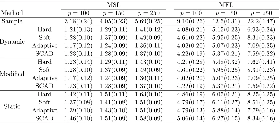
Table 1: Average (standard error) MSLs and MFLs for Model 1

MSL MFL

Method p= 100 p= 150 p= 250 p= 100 p= 150 p= 250

Sample 3.18(0.24) 4.05(0.23) 5.69(0.25) 9.10(0.26) 13.5(0.31) 22.2(0.47)

Dynamic

Hard 1.21(0.13) 1.29(0.11) 1.41(0.12) 4.08(0.21) 5.15(0.23) 6.93(0.24) Soft 1.28(0.10) 1.37(0.09) 1.49(0.09) 4.61(0.22) 5.95(0.25) 8.31(0.23) Adaptive 1.17(0.12) 1.24(0.09) 1.36(0.11) 4.02(0.20) 5.07(0.23) 7.09(0.25) SCAD 1.23(0.11) 1.28(0.09) 1.37(0.10) 4.22(0.19) 5.37(0.21) 7.59(0.22)

Modified

Static

computed from an independent data. We adopt this idea. Specifically, we divide the original

sample into two samples at random of size n1 andn2, wheren1 =n(1−_log1_n) and n2 = _logn_n, and

repeat this N1 times. Let ˆΣ1,s(u) and ˆΣ2,s(u) be the empirical dynamic covariance estimators

according to (2) based on n1 and n2 observations respectively with the bandwidth selected by

the subset-y-variables cross validation. Given u, we select the thresholding parameter ˆλ(u) by

minimizing

R(λ, u) := 1

N1

X

s=1

||sλ( ˆΣ1,s(u))−Σˆ2,s(u)||2F,

where ||M||2

F = tr(M MT) is the squared Frobenius norm of a matrix.

4 Numerical Studies

In this section we investigate the finite sample performance of the proposed procedure with Monte

Carlo simulation studies. We compare our method to the static covariance matrix estimates

in Rothman et al. (2009) when generalized thresholding, including hard, soft, adaptive lasso,

and SCAD thresholding, is considered. We also include the modified estimator ˆΣM(u) that

guarantees positive definiteness and the empirical sample dynamic covariance matrix in (2) for

comparison purposes. Throughout the numerical demonstration, the Gaussian kernel function

K(a) = _√1

2π exp(−a

(15)

[image:15.612.61.532.61.269.2]

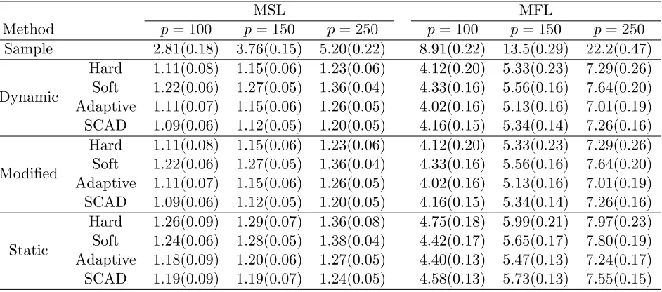
Table 2: Average (standard error) MSLs and MFLs for Model 2

MSL MFL

Method p= 100 p= 150 p= 250 p= 100 p= 150 p= 250

Sample 2.81(0.18) 3.76(0.15) 5.20(0.22) 8.91(0.22) 13.5(0.29) 22.2(0.47)

Dynamic

Modified

Static

4.1 Simulation studies

Study 1.

We consider two dynamic covariance matrices in this study to investigate the accuracy of our

proposed estimating approach in terms of the spectral loss and the Frobenius loss of a matrix.

Model 1: (Dynamic banded covariance matrices). Let Σ(u) ={σij(u)}1≤i,j≤p,whereσij(u) =

exp(u/2)[{φ(u) + 0.1}I(|i−j|= 1) +φ(u)I(|i−j|= 2) +I(i=j)] and φ(u) is the density of the

standard normal distribution.

Model 2: (Dynamic AR(1) covariance model). Let Σ(u) = {σij(u)}1≤i,j≤p, where σij(u) =

exp(u/2)φ(u)|i−j|_.

Model 2 is not sparse, although many of the entries in Σ(u) are close to zero for large p. This

model is used to assess the accuracy of the sparse DCMs for approximating non-sparse matrices.

For each covariance model, we generate 50 datasets, each consisting of n = 150

observa-tions. We sample Ui, i = 1,· · · , n, independently from the uniform distribution with support

[−1,1]. The response variable is generated according to Yi ∼ N(0,Σ(Ui)), i = 1,· · · , n, for

p = 100,150, or 250, respectively. The k and N in the subset-y-variables cross-validation

are set to be [p/12] and p, respectively, with [p/12] denoting the largest integer no greater

(16)

[image:16.612.56.539.74.434.2]

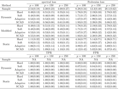
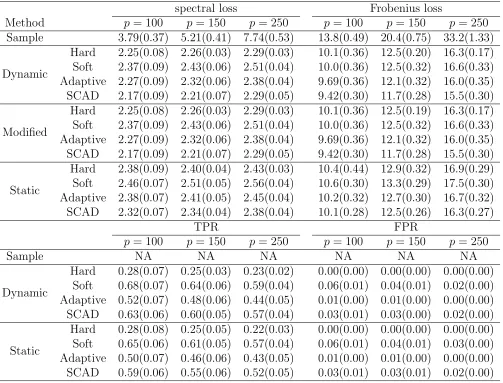
Table 3: Average (standard error) spectral loss, Frobenius loss, TPR and FPR when U =−0.75 for Model 3 in Study 2

spectral loss Frobenius loss

Method p= 100 p= 150 p= 250 p= 100 p= 150 p= 250

Sample 2.54(0.18) 3.30(0.23) 4.68(0.27) 8.28(0.34) 12.3(0.48) 20.1(0.62)

Dynamic

Modified

Static

TPR FPR

p= 100 p= 150 p= 250 p= 100 p= 150 p= 250

Sample NA NA NA NA NA NA

Dynamic

Static

spectral and Frobenius losses as the criteria to compare the estimators produced by various

approaches. Specifically, for each dataset, we estimate the DCMs at the following 20 points

ui ∈ A={−0.95,−0.85,· · · ,−0.05,0.05,0.15,· · · ,0.85,0.95}. Then for each method, we

calcu-late the medians of 20 spectral and Frobenius losses, defined as

Median Spectral Loss = median{5S(ui), i= 1,· · ·,20},

Median Frobenius Loss = median{5F(ui), i= 1,· · ·,20},

where 5S(u) = max1≤j≤p|λj{Σ(ˆ u)−Σ(u)}| and 5F(u) =

q

trace[{Σ(ˆ u)−Σ(u)}2_{] are spectral}

loss and Frobenius loss, respectively. For brevity, the two losses, Median Spectral Loss and

Median Frobenius Loss, are referred to as MSL and MFL, respectively.

(17)

[image:17.612.56.539.74.435.2]

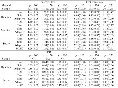
Table 4: Average (standard error) spectral loss, Frobenius loss, TPR and FPR when U = 0.25 for Model 3 in Study 2

Method p= 100 p= 150 p= 250 p= 100 p= 150 p= 250

Sample 3.03(0.26) 4.11(0.26) 6.01(0.35) 10.8(0.32) 15.9(0.39) 26.1(0.68)

Dynamic

Modified

Static

TPR FPR

p= 100 p= 150 p= 250 p= 100 p= 150 p= 250

Dynamic

Static

estimators of the dynamic covariance matrices in Model 1 and Model 2, respectively. Here,

Sample represents the sample conditional covariance estimate in (2). Several conclusions can be

drawn from Table 1 and Table 2. First, there is a drastic improvement in accuracy by using

thresholded estimators over the kernel smoothed conditional covariance matrix in (2), and this

improvement increases with dimensionp. Second, as is expected, our proposed estimating method

produces more accurate estimators than the static covariance estimation approach independent

of the thresholding rule used. Third, the modified estimators perform similarly as the unmodified

dynamic estimates. However, we observe that the unmodified estimate is not positive definite

sometimes. For example, whenn = 100 in Model 2, we observe that about 0.6% of the estimated

(18)

Study 2.

In this study, we consider a dynamic covariance model whose sparsity pattern varies as a function

of the covariateU. The purpose of this study is to assess the ability of our proposed method for

recovering the varying sparsity, evaluated via the true positive rate (TPR) and the false positive

rate (FPR), defined as

T P R(u) = #{(i, j) :sλn(u)(ˆσij(u))6= 0 and σij(u)6= 0}

#{(i, j) :σij(u)6= 0}

,

F P R(u) = #{(i, j) :sλn(u)(ˆσij(u))6= 0 and σij(u) = 0} #{(i, j) :σij(u) = 0}

,

respectively (Rothman et al., 2009). For each given point u, we also evaluate the estimation

accuracy of various approaches in terms of the spectral loss and the Frobenius loss.

Model 3: (Varying-sparsity covariance model) Let Σ(u) = {σij(u)}1≤i,j≤p, where

σij(u) = exp(u/2)

h

0.5 exp{− (u−0.25)

2

0.752₋₍_u₋₀_.₂₅₎2}I(−0.5≤u≤1)I(|i−j|= 1)

+0.4 exp{− (u−0.65)

2

0.352₋₍_u₋₀_.₆₅₎2}I(0.3≤u≤1)I(|i−j|= 2) +I(i=j)

i

.

For this model, we assess the estimated covariance matrices at three points{−0.75,0.25,0.65}.

Note that from the data generating process, the sparsity of this dynamic covariance model varies

with the value of U, and that the covariance matrices at −0.75, 0.25 and 0.65 are diagonal,

tridiagonal and five-diagonal respectively.

The data is generated following the procedure in Study 1. We report the spectral losses,

Frobenius losses, TPRs and FPRs in Table 3, Table 4 and Table 5 at point −0.75, 0.25 and

0.65, respectively. In these tables, “NA” means “not applicable”. Since the modified dynamic

covariance estimator does not change the sparsity, we do not report the performance of this

method for sparsity identification. The following conclusions can be drawn from the three tables.

First, the accuracy statement in terms of the spectral loss and Frobenius loss made in Study

1 continues to hold in this study. Second, for each thresholding rule, our proposed dynamic

(19)

[image:19.612.58.561.216.599.2]

Table 5: Average (standard error) spectral loss, Frobenius loss, TPR and FPR when U = 0.65 for Model 3 in Study 2

Method p= 100 p= 150 p= 250 p= 100 p= 150 p= 250

Sample 3.79(0.37) 5.21(0.41) 7.74(0.53) 13.8(0.49) 20.4(0.75) 33.2(1.33)

Dynamic

Modified

Static

TPR FPR

p= 100 p= 150 p= 250 p= 100 p= 150 p= 250

Dynamic

Static

(20)

SCAD thresholding rules seems to have higher TPRs than using the hard and the adaptive

thresholding rules.

Study 3.

In this study, we demonstrate the effectiveness of our proposed method for estimating a dynamic

covariance model whose positions of the nonzero elements varied as a function of the covariate

U.

Model 4: (Varying-nonzero-position covariance model) The dynamic covariance model is

similar to the random graph model in Zhou et al. (2010). Specifically, we examine 9 time points

{−1,−0.75,−0.5,−0.25,0,0.25,0.5,0.75,1}. LetR(u) be the correlation matrix at pointu. We

randomly choose p entries {rij : i = 2,· · · , p;j < i} of R(−1) such that each of these p

ele-ments was a random variable generated from the uniform distribution with support [0.1,0.3].

The other correlations in R(−1) are all set to zero. For each of the other 8 time points

{−0.75,−0.5,−0.25,0,0.25,0.5,0.75,1}, we change p/10 existing nonzero correlations to zero

and add p/10 new nonzero correlations. For each of the p/10 new entries having nonzero

cor-relations, we choose a target correlation, and the correlation on the entry is gradually changed

to ensure smoothness. Similarly, for each of the p/10 entries to be set as zero, the correlation

decays to zero gradually. Thus, there exist p+p/10 nonzero correlations and there existp/5

cor-relations that varied smoothly. The covariance matrix is then set as exp(u/2)R(u). We generate

data following the procedure in Study 1 with n = 100 or n = 150. The results for estimating

the covariance matrix at point U =−1 (Zhou et al., 2010) are reported in Table 6 for n = 150

and Table 7 for n = 100. We find that the proposed method performs better than the sample

estimates and the static estimates in terms of the spectral loss, Frobenius loss and TPR.

Finally, we investigate the performance of the proposed bandwidth selection procedure using

the model in this study. For a given bandwidth parameter h, our proposed estimator of Σ(u)

is denoted as sλn(u)( ˆΣ(u;h)). The oracle that knows the true dynamic covariance matrix Σ(u)

prefers to select the bandwidth parameterh(i.e.,horacle) that minimizesPn_i₌₁||sλn(Ui)( ˆΣ(Ui;h))−

Σ(Ui)||F, where || · ||F is the Frobenius loss. The bandwidth parameter selected by our

(21)

[image:21.612.56.570.217.599.2]

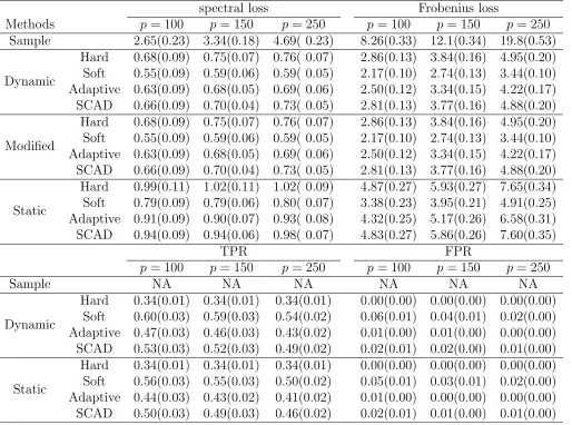
Table 6: Average (standard error) spectral loss, Frobenius loss, TPR and FPR whenU =−1 for Model 4 in Study 3 with n= 150

Methods p= 100 p= 150 p= 250 p= 100 p= 150 p= 250

Sample 2.65(0.23) 3.34(0.18) 4.69( 0.23) 8.26(0.33) 12.1(0.34) 19.8(0.53)

Dynamic

Hard 0.68(0.09) 0.75(0.07) 0.76( 0.07) 2.86(0.13) 3.84(0.16) 4.95(0.20) Soft 0.55(0.09) 0.59(0.06) 0.59( 0.05) 2.17(0.10) 2.74(0.13) 3.44(0.10) Adaptive 0.63(0.09) 0.68(0.05) 0.69( 0.06) 2.50(0.12) 3.34(0.15) 4.22(0.17) SCAD 0.66(0.09) 0.70(0.04) 0.73( 0.05) 2.81(0.13) 3.77(0.16) 4.88(0.20)

Modified

Static

TPR FPR

p= 100 p= 150 p= 250 p= 100 p= 150 p= 250

Dynamic

Static

(22)

[image:22.612.56.564.74.458.2]

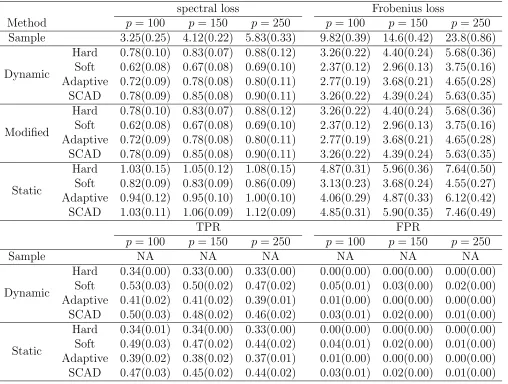
Table 7: Average (standard error) spectral loss, Frobenius loss, TPR and FPR whenU =−1 for Model 4 in Study 3 with n= 100

Method p= 100 p= 150 p= 250 p= 100 p= 150 p= 250

Sample 3.25(0.25) 4.12(0.22) 5.83(0.33) 9.82(0.39) 14.6(0.42) 23.8(0.86)

Dynamic

Modified

Static

TPR FPR

p= 100 p= 150 p= 250 p= 100 p= 150 p= 250

Dynamic

Static

horacle|/horacle as the criterion to measure the performance of hCV. Setting p= 100, we explore

the performance based on 50 simulations forn = 100,150 and 200, respectively. The medians of

50 absolute relative errors for sample sizes 100,150 and 200 are 0.12,0.06 and 0.01, respectively.

The percentages of absolute relative errors less than 20% for sample sizes 100, 150 and 200 are

0.82, 0.96, 0.98, respectively. It is concluded that the estimated bandwidth converges fast to its

oracle counterpart when the sample size grows.

4.2 Real data analysis

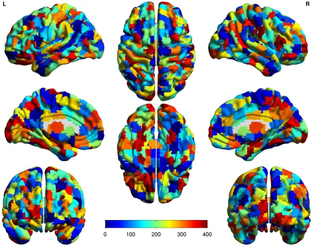
As an illustration, we apply the dynamic covariance method to the resting state fMRI data

obtained from the attention deficit hyperactivity disorder (ADHD) study conducted by New York

(23)

[image:23.612.151.457.45.288.2]

Figure 1: The ROIs from the CC400 functional parcellation atlases.

disorders and can continue through adulthood. Symptoms of ADHD include difficulty staying

focused and paying attention, difficulty controlling behavior, and over-activity. An ADHD patient

tends to have high variability in brain activities over time. Because fMRI measures brain activity

by detecting associated changes in blood flow through low frequency BOLD signal in the brain

(Biswal et al., 1995), it is believed that the temporally varying information in fMRI data may

provide insight into the fundamental workings of brain networks (Calhoun et al., 2014; Lindquist

et al., 2014). Thus, it is of great interest to study the dynamic changes of association among

different regions of interest (ROIs) of the brain for an ADHD patient at the resting state. For

this dataset, we examine the so-called CC400 ROI atlases with 351 ROIs derived by functionally

parcellating the resting state data as discussed in Craddock et al. (2012). An illustration of these

ROIs is found in Figure 1.

The experiment included 222 children and adolescents. We focus on Individual 0010001. The

BOLD signals of p = 351 ROIs of the brain were recorded over n = 172 scans equally spaced

in time. We treat the time as the index variables U after normalizing the 172 scanning time

points onto [0,1]. The main aim is to assess how the correlations of BOLD signals change with

the scanning time, as changing correlations can illustrate the existence of distinctive temporal

(24)

0.0 0.2 0.4 0.6 0.8 1.0

−0.5

0.0

0.5

Time

Correlation

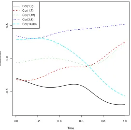
[image:24.612.160.431.64.331.2]

Cor(1,2) Cor(1,7) Cor(1,12) Cor(3,4) Cor(14,30)

Figure 2: Selected entries of the correlation matrix as functions of time using (2) for the ADHD data. Cor(k, l) represents the (k, l)-th element of the correlation matrix.

covariance estimating method and compare it to the static method in Rothman et al. (2009).

We first obtain the sample covariance estimate as defined in (2), and plot selected entries of

this matrix in Figure 2. We can see that the correlations of BOLD signals for different pairs of

ROIs vary with time. For example, the entries (1,7) and (14,30) as functions of the time change

signs, one from negative to positive and one from positive to negative. Entries (1,2) and (3,4)

seem to remain negative and positive respectively over the entire time, while entry (1,12) is very

close to zero before becoming positive. As discussed in the Introduction, a test of the equality

of the two covariance matrices, one for the first 86 scans and the other for the last 86 scans, is

rejected. These motivate the use of the proposed dynamic covariance method. For the dynamic

sparse estimates, we only report the results using the soft thresholding rule, since simulation

studies indicate that this thresholding rule performs satisfactorily in recovering the true sparsity

of the covariance matrices. We examine the estimated dynamic covariance matrices at the 50-th,

90-th and 130-th scans.

(25)

[image:25.612.150.448.62.150.2]

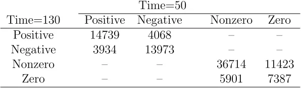
Table 8: Qualitative summary of the estimated correlations at time 50 and 130 Time=50

Time=130 Positive Negative Nonzero Zero

Positive 14739 4068 – –

Negative 3934 13973 – –

Nonzero – – 36714 11423

Zero – – 5901 7387

in Figure 3 (a), (b) and (c) for time 50, 90 and 130 respectively. We can see a clear varying

pattern in panel (a)–(c), as compared to the static covariance matrix estimate in panel (e).

To appreciate the dynamic characteristics of the BOLD signals, in panel (d), we use K-means

clustering to cluster the 351 time series, one from each ROI, with K = 10, and plot these ten

centroids. We can see different correlation patterns for the BOLD signals during different time

periods, indicating the need for dynamically capturing the time varying phenomenon.

We comment on the dynamic nature of the three estimated matrices. The matrices at time

50, 90 and 130 have 42615, 46778 and 48137 non-zero correlations, respectively. That is, the

covariance matrix at time = 130 is denser than those at time = 50 and 90. This tells that the

sparsity of the covariance varies with time. Moreover, the positions of the nonzero (or zero)

correlations change with time. For example, as Table 8 shows, there are 7387 and 36714 entries

(correlations) of the estimated covariance matrices at time = 50 and 130 to be simultaneously

zero and nonzero, respectively. However, there are 5901 entries (correlations) that are nonzero in

the estimated covariance matrix at time = 50 but are zero in the estimated matrix at time = 130.

There are 11423 entries (correlations) that are zero in the estimated matrix at time = 50 but

are zero in the estimated matrix at time = 130. Furthermore, the signs of the correlations are

time varying. As Table 8 shows, the numbers of the entries (correlations) of the two estimated

covariance matrices being simultaneously positive and negative are 14739 and 13973, respectively.

Meanwhile, there are 4068 entries (correlations) that are negative in the estimated covariance

matrix at time = 50 but are positive in the estimated matrix at time = 130. And there are 3934

entries (correlations) that are positive in the estimated covariance matrix at time = 50 but are

negative in the estimated matrix at time = 130. We found that, at time = 50, 2 ROIs have

more than 325 associations with other ROIs, and that 8 ROIs have fewer than 10 associations

(26)

0 10 20 30

−1.0 −0.5 0.0 0.5 1.0

Correlation

(a)

0 10 20 30

−1.0 −0.5 0.0 0.5 1.0

Correlation

(b)

0 10 20 30

−1.0 −0.5 0.0 0.5 1.0

Correlation

(c)

0.0 0.2 0.4 0.6 0.8 1.0

−1.0

0.0

1.0

Time

BOLD Signal

(a) t=50/172 (b) t=90/172 (c) t=130/172

(d)

0 10 20 30

−1.0 −0.5 0.0 0.5 1.0

Correlation

[image:26.612.57.559.89.629.2]

(e)

(27)

becomes 11, and the number of the ROIs having fewer than 10 associations is 3, indicating that

there are more active ROIs at this time. However, the static covariance estimating method can

not show these dynamics.

As brain activities are often measured through low frequency BOLD signals in the brain,

our model indicates that the correlations of different areas of the brain varied over time, which

coincides with the high variability of brain function for an ADHD patient and makes sense for

the purpose of locating the ADHD pathology.

5 Discussion

We study for the first time a novel uniform theory of the dynamic covariance model that combines

the strength of kernel smoothing and modelling sparsity in high dimensional covariances. Our

numerical results show that our proposed method can capture dynamic behaviors of these varying

matrices and outperforms its competitors. We are currently studying similar uniform theory for

high dimensional regression and classification where dynamics are incorporated.

We identify several directions for future study. First, the kernel smoothing employed in this

paper uses local constant fitting. It is interesting to study local linear models that is known

to reduce bias (Fan and Gijbels, 1996). A first step was taken by Chen and Leng (2015) when

the dimensionality is fixed, but more research is warranted. Second, it is of great interest to

develop more adaptive thresholding rules such as those in Cai and Liu (2011). A difficulty in

extending our method in that direction is that the sample dynamic covariance matrix in (2) is

biased entrywise, unlike the sample static covariance matrix in Cai and Liu (2011). Third, it is of

great interest to study a new notion of rank-based estimation of a large dimensional covariance

matrix in a dynamic setting (Liu et al., 2012; Xue and Zou, 2012) that is more robust to the

distributional assumption of the variables. Fourth, it is possible to study dynamic estimation

of the inverse of a covariance matrix that elucidates conditional independence structures among

the variables (Yuan and Lin, 2007). These topics are beyond the scope of the current paper and

(28)

Appendix

Lemma 4. Under Conditions (a)–(d), suppose that (3) is satisfied and sup_u∈Ωσii(u)< M2 <∞

for all i. If x >0 and x→0 as n → ∞, we have, for 1≤i≤n, 1≤j ≤p and 1≤k ≤p,

EexK(Ui

−u

h )YijYik _<_∞

for each u∈Ω.

Proof. When n is large enough, we have

EexYijYik _{= 1 +}_xEY

ijYik+

x2 2 EY

2

ijY

2

ik+

x3 3!EY

3

ijY

3

ik+· · ·

≤ 1 +xEY_ij2+ x 2

2EY 4

ij +

x3 3!EY

6

ij +· · ·

+1 +xEY_ik2 +x 2

2 EY 4

ik+

x3

3!EY 6

ik+· · ·

= EexYij2 +EexYik2 <∞.

By simple calculation, it is seen Ee|xYijYik| _<∞_. _{Due to the boundedness of the kernel function}

K(·), we obtain Ee|xK(Ui_h−u)YijYik|_<∞_._{The result follows.}

Define Wijk(u, h) :=K{(Ui−u)/h}YijYik−EK{(Ui−u)/h}YijYik, for 1≤i≤n, 1≤j ≤p

and 1≤k ≤p. By Lemma 4, we easily have the following lemma.

Lemma 5. Under Conditions (a)–(d), if (3) holds and sup_u_∈_Ωσii(u)< M2 <∞ for all i, then,

if x > 0 and x→ 0 as n → ∞, there exists a positive constant gi =O(var(Wijk(u, h)) =O(h),

which does not depend on u, such that

Eexp{xWijk(u, h)} ≤exp{gix2}

for each u∈Ω.

The exponential convergence rate for|1

n

Pn

i=1Kh(Ui−u)YijYik−EKh(Ui−u)YijYik|is impor-tant for deriving our theorems. First, we obtain its point-wise convergence rate in the following

(29)

Lemma 6. Under Conditions (a)–(d), suppose that (3) holds and sup_u∈Ωσii(u)< M2 <∞ for

all i. If λn →0, there exists a constant C >0, which does not depend on u, such that

P 1 n n X i=1

Kh(Ui−u)YijYik−EKh(Ui−u)YijYik

≥λn

≤2 exp{−Cnhλ2_n}

for each u∈Ω.

Proof. Define G := Pn

i=1gi = O(nh). By Lemma 5, for x > 0 and x → 0 as n → ∞, we have

P

n

X

i=1

Wijk(u, h)≥λn

≤ exp{−xλn}Eexp{x n

X

i=1

Wijk(u, h)}

= exp{−xλn}ΠniEexp{xWijk(u, h)}

≤ exp{−λnx+Gx2}. (6)

Note that (6) is maximized when x=λn/2G→ 0 and that the maximizer is exp{−

λ2

n

4G}. Thus,

there exists a positive constant C such that

Pn1 n

n

X

i=1

o

≥λn

≤exp{−Cnhλ2_n}.

Similarly, we obtain

Pn1 n

n

X

i=1

Kh(Ui −u)YijYik−EKh(Ui−u)YijYik

o

≤ −λn

≤exp{−Cnhλ2_n}.

Combining the above two equations, the result is established.

We discuss the uniform exponential convergence rate for|1

n

Pn

i=1Kh(Ui−u)YijYik−E(YijYik|U =

u)f(u)|, which plays an important role in deriving our theorems.

Lemma 7. Under Conditions (a)–(d), suppose that (3) holds, sup_u|K0(u)| < M5 < ∞ and

sup_u_∈_Ωσii(u) < M2 < ∞ for all i. For sufficient large M

0

, if λn = M

0

(

q

logp

nh +h

2√_log_p₎_,

logp

nh →0 and h

4_log_p_→₀_{, there exist} _C

1 >0 and C2 >0 such that

Psup

u∈Ω

1 n n X i=1

Kh(Ui −u)YijYik−E(YijYik|U =u)f(u)

≥λn

(30)

Proof. Without loss of generality, we let Ω = [a, b]. Decompose [a, b] =∪qn

l=1[un,l−rn, un,l+rn],

which contains qn intervals of length 2rn. That is 2qnrn =b−a. Then,

sup

u∈[a,b]

1 n n X i=1

≤ max 1≤l≤qn

1 n n X i=1

Kh{Ui−un,l}YijYik−EKh{Ui−un,l}YijYik

+ max 1≤l≤qn

sup

u∈[un,l−rn,un,l+rn]

1 n n X i=1

Kh(Ui−u)YijYik−

1

n

X

i=1

Kh{Ui−un,l}YijYik

− {EKh(Ui−u)YijYik−EKh(Ui−un,l)YijYik}

.

Let rn =h4, then qn = b₂−_ha4. Let λn =M 0

(

q

logp

nh +h

2√_log_p_{), where} _M0

is sufficiently large,

logp

nh → 0 and h

4_log_p _→ _{0. Define} _B

1 = {ω : max1≤l≤qnsupu∈[un,l−rn,un,l+rn]|

1

n

Pn

i=1Kh(Ui −

u)YijYik − _n1

Pn

i=1Kh(Ui −un,l)YijYik − {EKh(Ui−u)YijYik −EKh(Ui −un,l)YijYik}| < λn/3}

and B2 =B1C. By Taylor’s expansion, we have

sup

1 n n X i=1

Kh(Ui−u)YijYik−

1

n

X

i=1

Kh(Ui−un,l)YijYik

≤h4 sup

1 nh2 n X i=1 n

K0(Ui−un,l+Ri(un,l−u)

h )YijYik

−EK0(Ui−un,l+Ri(un,l−u)

h )YijYik

o

, (7)

where 0 < Ri < 1 is a random scalar depending on Ui, for i = 1,· · · , n. Since supu|K

0

(u)| <

M5 <∞, (7) is bounded by

h2_M 5

n

X

i=1

(Y_ij2 +Y_ik2) +h2M5(EY_ij2+EY_ik2). (8)

(31)

A (for all l) such that

P sup

1 n n X i=1

Kh(Ui −u)YijYik−

1

n

X

i=1

Kh(Ui−un,l)YijYik

≥λn/3

≤2 exp{−An h4 λ

2

n}.

Thus, we obtain immediately

P(B2) = P

max 1≤l≤qn

sup

1 n n X i=1

Kh(Ui−u)YijYik−

1

n

X

i=1

Kh(Ui−un,l)YijYik

≥λn/3

= qn max

1≤l≤qn

P sup

1 n n X i=1

Kh(Ui−u)YijYik−

1

n

X

i=1

Kh(Ui −un,l)YijYik

≥λn/3

≤ 2qnexp{−

An h4 λ

2

n}. (9)

Note

P

sup

u∈[a,b]

1 n n X i=1

≥λn

≤Pn sup

u∈[a,b]

1 n n X i=1

≥λn

o

∩ B1

+Pn sup

u∈[a,b]

1 n n X i=1

≥λn

o

∩ B2

:=J1+J2.

We know that J1 is bounded (using Lemma 6) as

P max 1≤l≤qn

1 n n X i=1

Kh{Ui−un,l}YijYik−EKh{Ui−un,l}YijYik

≥(λn−λn/3)

≤qn max

1≤l≤qn

P 1 n n X i=1

Kh{Ui −un,l}YijYik−EKh{Ui −un,l}YijYik

≥λn/2

(32)

and that J2 is bounded by (9). Therefore, for large enoughn,

P sup

u∈[a,b]

1 n n X i=1

≥λn

≤4qnexp{−Cnhλ2n/4} ≤

2(b−a)

h4 exp{−Cnhλ 2

n/4}.

It is well known that (Pagan and Ullah, 1999; Fan and Huang, 2005)

sup

u∈[a,b]

EKh(Ui−u)YijYik−E(YijYik|U =u)f(u)

=O(h

2₎_.

Since

sup

u∈[a,b]

1 n n X i=1

Kh(Ui−u)YijYik−E(YijYik|U =u)f(u)

≤ sup

u∈[a,b]

1 n n X i=1

+ sup

u∈[a,b]

EKh(Ui−u)YijYik−E(YijYik|U =u)f(u)

and λn h2, we have immediately

P sup

u∈[a,b]

1 n n X i=1

Kh(Ui−u)YijYik−E(YijYik|U =u)f(u)

≥λn

≤P sup

u∈[a,b]

1 n n X i=1

≥λn/2

≤ 2(b−a)

h4 exp{−Cnhλ 2

n/16}.

Letting C1 =C/16 and C2 = 2(b−a), we obtain the conclusion.

Remark 3. We now outline the main steps of our proofs. Along the way, we highlight the

main theoretical innovations and comment that existing results in the literature may not apply

to the high-dimensional problems we are interested in studying. In the first step, we obtain the

exponential convergence rate of|1

n

Pn

i=1Kh(Ui−u)YijYik−EKh(Ui−u)YijYik|in Lemma 6 for each

u on a discrete grid. After decomposing Ω, we transform the uniform exponential convergence

(33)

6. The exponential uniform convergence result of the kernel estimators in Lemma 7, essential

for establishing the main conclusions of the paper, plays an important role in deriving the rates

of convergence in Theorem 1 and Proposition 3 as well as the result in Theorem 2, when one

deals with problems with the dimensionality exponentially high in relation to the sample size.

In contrast, Einmahl and Mason (2005) used the exponential inequality of Talagrand (1994) to

construct the uniform exponential convergence rate. According to their arguments, the right

hand side of (7) should be much larger than h−4exp{−C1nhλ2n}. This indicates that the result

implied by the theorems in Einmahl and Mason (2005) is not enough for deriving the uniform

convergence results in our paper and thus does not apply to the challenging high-dimensional

setup.

Remark 4. To facilitate the proof of Lemma 7, we assume sup_u|K0(u)|< M5 <∞. However,

this does not mean that some commonly used kernel functions (e.g., the boxcar kernel) can not

be used. We now examine the boxcar kernel specifically. WriteK(u) = 1₂I(|u| ≤1) and note

sup

1 n n X i=1

Kh(Ui−u)YijYik−

1

n

X

i=1

Kh(Ui−un,l)YijYik

≤ 1

2_u∈[un,lsup−rn,un,l]

1 n n X i=1 1

hI{Ui ∈[u+h, un,l+h]}YijYik−E

1

hI{Ui ∈[u+h, un,l+h]}YijYik

+1

2u∈[un,lsup−rn,un,l]

1 n n X i=1 1

hI{Ui ∈[u−h, un,l−h]}YijYik−E

1

hI{Ui ∈[u−h, un,l−h]}YijYik

+1

2u∈[un,lsup,un,l+rn]

1 n n X i=1 1

hI{Ui ∈[un,l+h, u+h]}YijYik−E

1

hI{Ui ∈[un,l+h, u+h]}YijYik

+1

2u∈[un,lsup,un,l+rn]

1 n n X i=1 1

hI{Ui ∈[un,l−h, u−h]}YijYik−E

1

hI{Ui ∈[un,l−h, u−h]}YijYik

:= A1+A2 +A3+A4. (10)

We have

A1 ≤

1 n n X i=1 1

hI{Ui ∈[un,l+h−rn, un,l+h]}(Y

2

ij +Y

2

ik)

+|E{1

hI{Ui ∈[un,l+h−rn, un,l+h]}(Y

2

ij +Y

2

ik)