warwick.ac.uk/lib-publications
A Thesis Submitted for the Degree of PhD at the University of Warwick
Permanent WRAP URL:
http://wrap.warwick.ac.uk/90155
Copyright and reuse:
This thesis is made available online and is protected by original copyright. Please scroll down to view the document itself.
Please refer to the repository record for this item for information to help you to cite it. Our policy information is available from the repository home page.
Value is context dependent: On comparison processes and rank order in choice
and judgment
by
Emina Canic
Thesis submitted in fulfillment of the requirements for the degree of Doctor of Philosophy in Psychology
University of Warwick, Department of Psychology
Table of contents
List of Tables ... v
List of Figures ... vi
Acknowledgements ... x
Declarations ... xi
Abstract ... xii
Chapter 1: Models of Choice ... 1
Chapter 2: Examining how utility and weighting functions get their shapes: A multi-level, quasi-adversarial, replication ... 28
SRH’s (2015) study: setup, motivation, methodology and results ... 31
Four Level replication ... 38
Level 1: Replication by reanalyzing the original data ... 38
Level 2: Replication by using a new subject pool ... 40
Level 3: Replication by implementing a new design ... 46
Level 4: Meta-analysis ... 53
Conclusion ... 56
Chapter 3: Choices remain context sensitive, even under high cognitive load ... 58
How do intelligence and working memory capacity relate to each other? ... 58
Cognitiveload is associated with more random responding, not more risk aversion ... 64
Decision by sampling predicts cognitive load will reduce sensitivity to the distribution of attribute values ... 65
Experimental Programme ... 66
Experiment 1A ... 67
Method ... 67
Results and discussion ... 68
Experiment 1B ... 70
Method ... 70
Results and discussion ... 70
Experiment 2 ... 72
Method ... 72
Results and discussion ... 73
Meta-analysis ... 74
The SRH effect remains under high cognitive load ... 74
Risk aversion does not increase under high cognitive load ... 76
Cognitive load decreases consistent choice behavior a little ... 77
General Discussion ... 79
Chapter 4: Stewart & Reimers (2008): More evidence for the rank hypothesis in judgment and choice ... 83
Behavioral Evidence ... 86
Neurophysiological Evidence ... 96
Experiments SR1A and SR1B ... 100
Experiments SR2A to SR2E ... 102
Conclusion ... 106
Chapter 5: Affective evaluation of monetary outcomes is unaffected by rank position ... 108
Kassam, Morewedge, Gilbert, and Wilson’s (2011) experiments ... 108
Differential processing of positive and negative outcomes ... 112
Reanalysis of Kassam et al.’s Experiment 2: Winners too love money ... 116
Experiment 1 ... 116
Method ... 117
Results ... 118
Testing a decision by sampling account of the Kassam et al. effect ... 120
Experiment 2 ... 123
Experiment 2A ... 124
Experiment 2B ... 126
Experiment 2C ... 128
Meta-analysis ... 129
Conclusion ... 132
Chapter 6: A Negative Zero is Better than a Positive Zero: The Mutable-Zero Effect and Category-Consistent Counterfactuals ... 134
The Any-Counterfactuals Hypothesis ... 135
The Category-Consistent-Counterfactuals Hypothesis ... 137
Method ... 139
Results and discussion ... 142
Experiment 2 ... 144
Method ... 144
Results and discussion ... 146
Experiment 3 ... 148
Method ... 148
Results and discussion ... 149
Meta-analysis ... 149
Main effect of M0 ... 150
Main effect of context ... 150
Context-by-M0 interaction ... 152
General Discussion ... 153
Chapter 7: Conclusion ... 160
Chapter 2 ... 160
Chapter 3 ... 162
Chapter 4 and 5 ... 163
Chapter 6 ... 167
Conclusion ... 168
References ... 170
Appendix A ... 190
List of Tables
Table 1.1. Choice phenomena and corresponding explanations of different accounts ... 4
Table 1.2. Options A and B result from merging Option A+ with A- and Option B+ with B-
respectively. The probabilities to win or lose are 25%. In the one-domain options, the
gambles offer a 50% chance of nothing ... 16
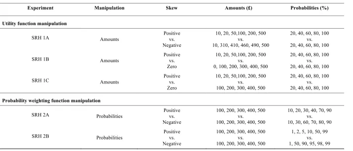
Table 2.1. Outline of the amounts and probabilities used in each SRH original experiment to
create the choice gambles ... 33
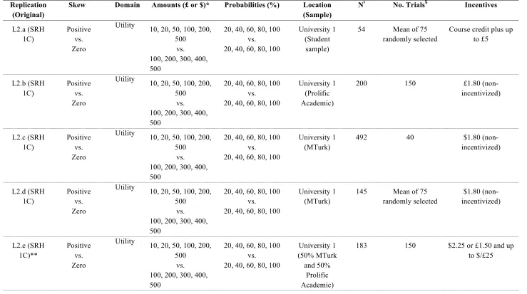
Table 2.2. Outline of the properties of all replication experiments from Level 2 ... 43
Table 2.3. Outline of the properties of all experiments from Level 3 ... 50
Table 4.1. Key features of experiments investigating context effects in judgment and choice . 87
Table 4.2. Experimental set-up in all five SR2 experiments ... 105
Table 6.1. Odds Ratios (OR) for choosing the M0 Option with 95% confidence interval ... 142
Table A1. Results from the SRH’s original analysis using SRH raw data with and without the
List of Figures
Figure 1.1. Prospect theory’s value and probability weighting functions ... 9
Figure 1.2. The left panel shows the predictions given participants experience the negative or
the positive condition. The right panel shows estimated value functions from real
choices under the according conditions ... 24
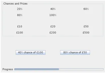
Figure 2.1. Interface used in SRH 1A. ... 35
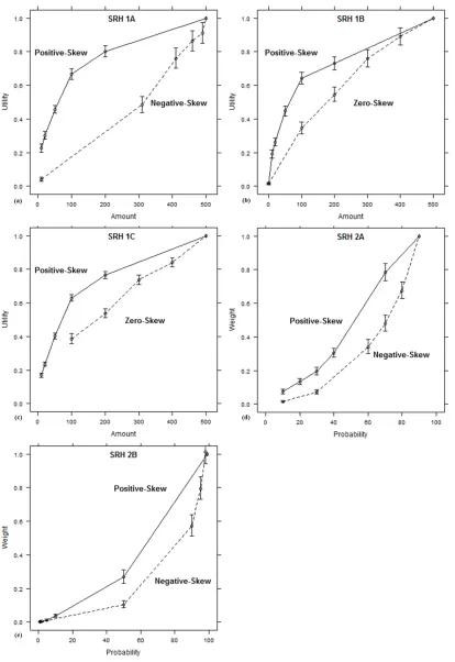
Figure 2.2. The revealed utility and probability weighting functions from SRH. Error bars are
95% confidence intervals. ... 37
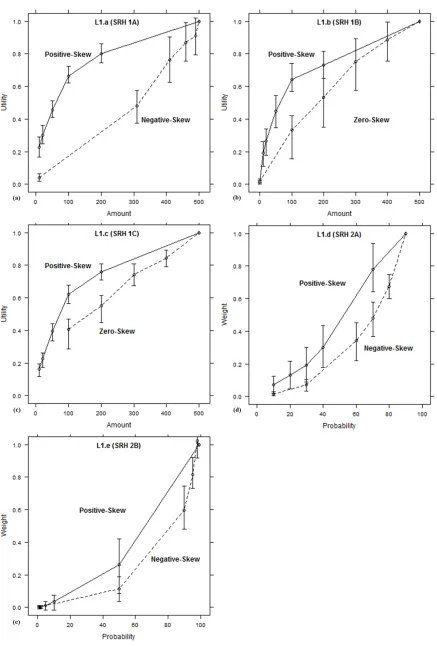
Figure 2.3. The revealed functions obtained from the replication analysis. Error bars are
95% confidence intervals. ... 41
Figure 2.4. Revealed functions from the replication experiments in Level 2. Error bars are
95% confidence intervals. ... 46
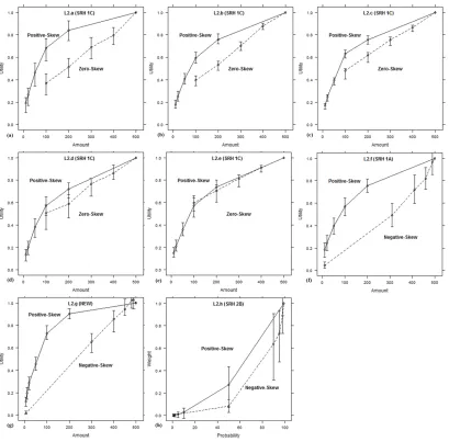
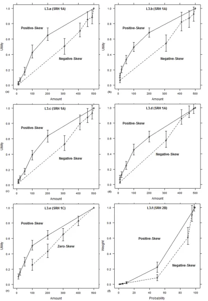
Figure 2.5. Revealed functions from the replications of SRH in Level 3 using a within-subjects
design. L3.a-L3.b involve flagged choices, L3.c-L3.f do not. Error bars are 95%
confidence intervals. ... 52
Figure 2.6.Meta-analysis results from Level 4. Mean Differences and 95% confidence
intervals are shown as a function of the experimental design for between-subjects, and
for flagged and non-flagged within-subject experiments. ... 55
Figure 3.1. Utility functions for Experiment 1A. Error bars are 95% confidence intervals. ... 70
Figure 3.2. Utility functions for Experiment 1B. Error bars are 95% confidence intervals. ... 71
Figure 3.3. Utility functions for Experiment 2. Error bars are 95% confidence intervals (CIs
are asymmetrical in the high-load conditions and are hidden under the dots and
triangles). ... 74
Figure 3.4. Mean Differences between the estimate for £200 (and $200 respectively) in the
positive-skew and the uniform conditions with 95% confidence intervals. Shown as a
Figure 3.5. Mean Differences between the estimate for £200 (and $200 respectively) in the
no/low load and the high load conditions with 95% confidence intervals, shown as a
function of distribution (Positive-skew or Uniform). ... 77
Figure 3.6. Mean Differences between estimates of γ in the no/low load and the high-load
conditions with 95% confidence intervals, shown as a function of distribution
(positive-skew or uniform conditions). Γs are consistently lower in the high-load than
the no/low-load conditions. ... 78
Figure 4.1. Mean attractiveness ratings with 95% confidence intervals for experiments SR1A
and SR1B. Gambles containing the critical attributes in the positive-skew conditions
were rated consistently higher than in the negative-skew conditions. ... 102
Figure 4.2. Odds ratios with 95% confidence intervals for experiments SR2A to SR2E and the
estimated overall effect size (blue diamond with width representing the 95% Cis).
Experiment features described in Table 4.2. ... 106
Figure 5.1. Redrawn mean ratings to different prizes with 95% confidence intervals from
Kassam et al.’s Experiment 1. ... 111
Figure 5.2. Redrawn mean ratings to prizes with 95% confidence intervals in critical trials
from Kassam et al.’s Experiment 2. We have presented the y-axis to cover the full 1-9
range. It demonstrates the effect of cognitive load on the sensitivity to the absolute
amount of the prize. ... 113
Figure 5.3. Means and 95% confidence intervals of positive affect for two filler trials of
Kassam et al.’s Experiment 2. The difference between the prize and its alternative
clearly matters for the valuation of the prize. ... 117
Figure 5.4. Means and 95% confidence intervals of positive affect after learning about the
prize money and its alternative separately for winners and losers in Experiment 1. The
same color and shape indicates equal prize money. ... 119
on the critical trial. ... 124
Figure 5.6. Means with 95% confidence intervals of positive affect ratings for the critical
trials in Experiments 2A-2C. Generally, there is no effect of either distribution or
cognitive load across experiments. ... 131
Figure 5.7. Mean differences with 95% confidence intervals between the fillers-outside and
the fillers-inside conditions, separately for low and high cognitive load of Experiments
2A-2C. ... 132
Figure 6.1. Experimental set-up of all nine experiments. In 1A and 1B participants click on
„Spin“ and watch the context items (in the grey box) pass by before it stops at either
„pay zero“ or „receive zero“, at which point the box blends in and turns green. In 1C
and 1D participants click on the blue cards in whichever order they prefer. The last
card they click on moves into the space where the „?“ was and turns green. Click here
to play the experiment with the spinner or here to play the experiment with the cards set-up. ... 140
Figure 6.2. Predicted choice proportions of M0 picks according to the three hypotheses. ... 142 Figure 6.3. Choice proportions of M0 picks and 95% confidence intervals for all nine
experiments. ... 151 Figure 6.4. Random effects meta-analysis to test the effect of the mutable zero category. Odds
ratios (OR) greater than 1 indicate an increase in the preference for the M0 Option
with „pay zero“ instead of „receive zero“. ... 152
Figure 6.5. Random effects meta-analysis on the effect of experimentally provided
counterfactuals for experiments with (1A-B and 3A-C) and without a labeled zero
(2A-D) separately. Odds ratios (OR) greater than 1 indicate an increase in the preference
for the M0 Option with pay-context instead of receive-context. ... 153
Figure 6.6. Meta-analysis to estimate the difference of the effect of experimentally provided
greater than 1 indicate that the difference between receive-context and pay-context
with a “receive zero” attribute is bigger than the difference between receive-context
and pay-context with a “pay zero” attribute. ... 154
Figure B1: Revealed functions from the replications of SRH in Level 3 using two models instead
Acknowledgements
I could not have written this thesis without my supervisor, Neil Stewart. Neil, I think you are awesome. Thank you for putting up with me. I am also grateful to Thomas Hills, who helped me develop research ideas and supported experiments in the field of moral cognition, and Elliot Ludvig, who helped me get published. Both Thomas and Elliot found time to listen and talk to me throughout my time as a PhD student.
Thank you to my parents, who were always there. To my sister and my friends at home, in England, Germany and the US: I am grateful for everything and I appreciate you being and staying in my life.
Declaration
I’m submitting this thesis to the University of Warwick. I have not submitted it anywhere else in any previous application for any other degree. I have completed this thesis independently and I have listed all references.
Abstract
In psychology as well as behavioral economics, it is well established that our choices and judgments are not just a function of the available options, but also of the context surrounding them. Several models have been brought forward to explain these context effects. We use the decision by sampling model (DbS; Stewart, Chater, & Brown, 2006) and investigate possible mechanisms that might lead to the relativity of judgment and choice. Stewart, Reimers and Harris (2015) demonstrated that shapes of utility and probability weighting functions could be manipulated by adjusting the distributions of outcomes and probabilities on offer. Chapter 2 reports a multi-level replication where we find that these effects are robust, but that DbS is unlikely to be the (sole) explanation for its origins. We conclude that problems with revealing utility functions from expected utility fits may be responsible for biasing the shapes of utility functions. Chapter 3 shows that reduced working memory capacity, as manipulated by cognitive load, does not reduce the effects found in Chapter 2. This further points away from a DbS explanation of the above findings. In Chapter 3, we also find that cognitive load has no impact on risk aversion, but find that choice consistency is reduced when working memory
1 Models of Choice
In recent years, some researchers have put forth process based theories in the judgment and decision making literature that stand in opposition to the neoclassical and sometimes even the descriptive theories. Whilst these process-based models have the aspiration to be a more realistic account of judgment and choice, they propose specific mechanisms–like comparison processes or rank ordering– that can be studied more thoroughly. In this thesis, I investigate to what degree comparison processes can drive the construction of choice under risk and the evaluation of prospects or sure outcomes. These insights will eventually help establish the role of comparison processes in human judgment and choice and can be afterwards
considered to inform policy, design learning applications or even build machines. In this chapter I will illustrate the breadth of accounts that have been offered to
account for some key choice phenomena, starting at prescriptive models of choice, moving on to descriptive models, and finally to process models. Even for a phenomenon as simple as risk aversion, I will review how some accounts appeal to the notion of diminishing marginal utility, some accounts appeal to probability weighting, and some accounts appeal to heuristic processes. Table 1.1 summarizes each phenomenon and the corresponding explanation in each account.
decision in the EV manner, it will maximize EV when the events are all added up. The crux here is that this argument is only really true, if people live infinitely, if there are infinite kinds of decisions and if there is an infinite number of people. However, none of these is the case (Baron, 2007). Why the EV should not be a sufficient criterion for the chooser and why it is not a description of people’s choices, is nicely demonstrated in the St. Petersburg paradox: If hypothetically one would offer somebody a lottery to win £2 pounds if a coin lands on tails on the first toss, £4 if it lands on tails on the second toss, £8 if it lands on the third toss etc., according to the EV criterion, everybody should be willing to pay an infinite amount of money to play the gamble, because the EV is infinite. However, to people this lottery is worth only a small amount of money. The fact that people would not pay a lot to play this lottery shows that EV alone is an insufficient criterion for describing choice under risk.
Daniel Bernoulli (1738) offered a resolution for the problem by introducing a (logarithmic) utility function, which transforms EV into expected utility (EU). The function takes into account the money a chooser already has when making a decision and assumes diminishing marginal utility. Diminishing marginal utility means that the utility of every extra unit of wealth is always positive, but is smaller than the utility of the previous unit. This
assumption solves the paradox, because while '("#$)2$
$ is infinite, ("# $
)()*2$ '
$ is finite at
or is indifferent, 2) when a person’s choices are transitive, i.e. if she likes A better than B, and B better than C, then she should like A better than C, 3) when stochastic dominance is met, i.e. when she chooses A over B, if A is better in at least one aspect and equally or at least as good in other aspects and finally 4) when her preferences are independent of the method they were elicited or of the way the options were described. These axioms form the basis of normative models.
Table 1.1
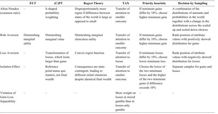
Choice phenomena and corresponding explanations of different accounts.
EUT (C)PT Regret Theory TAX Priority heuristic Decision by Sampling
Allais Paradox (common ratio)
– S-shaped
probability weighting
Disproportionately more regret if difference between states of the world is large as opposed to small
Transfer of attention to smaller outcome
If minimum gains differ by 10%, choose higher minimum gain
A combination of the distributions of amounts and probabilities in the world together with a change in the distributions across the scaled up and scaled down choices Risk Aversion Diminishing
marginal utility Diminishing marginal value Diminishing marginal choiceless utility Transfer of attention to smaller outcome
If minimum gains differ by 10%, choose higher minimum gain
Rank position of attribute values with positively skewed distribution for gains
Loss Aversion – Transformation of losses, which loom larger than gains
Convex regret function Transfer of attention to losses
If minimum losses differ by 10%, choose lower minimum loss
Rank position of attribute values with negatively skewed distribution for losses
Isolation Effect – Reference point/status quo matters, not final wealth
Consequences are state-contingent, leading to different initial situations despite identical final wealth
Transfer of attention to smaller outcome
Choose the lower of the two minimum losses and the higher of the two minimum gains if difference exceeds 10%
Separate samples for gains and losses
Violation of Gain-Loss Separability
– – – More weight on
losses in mixed gamble than in losses-only gamble
Yet, people often violate the rationality principles and do not choose the way
they ought to (Birnbaum, 2008, for a recent review). Hence EUT does not provide a
very accurate description of people’s choice behavior either. In the remainder of this
chapter, I will outline some of the key departures from EUT, and will start with a
classic example, the Allais paradox. What the St. Paradox is for EV is the Allais
paradox (Allais, 1953) for EUT: Consider the following choice options:
Option A: win 1Million for sure,
or
Option B: win 5 Million with a 10% chance, or win 1 Million with an 89% chance
and otherwise nothing.
People more often choose the safe option A, perhaps avoiding option B because they
are scared of the 1% chance of receiving nothing. Now consider these modified
options:
Option C: win 1 Million with an 11% chance and otherwise nothing,
or
Option D: win 5 Million with a 10% chance and otherwise nothing.
Now people more often choose the riskier Option D–as if they discount the difference
between the 10% and the 11% chance of winning. This preferential pattern describes
the common consequence effect. Removing an 89% chance of £1M from both options
A and B gives options C and D. Thus, to be consistent with EU, people must choose
either options A and C or B and D, because otherwise they violate independence from
irrelevant alternatives.
The common ratio effect–also first demonstrated by Allais–deals with an
EUT-inconsistency that considers probabilities instead of outcomes:
or
Option B: win £4000 with an 80% chance, otherwise nothing.
Again most people choose the safe Option A. On the other hand, when asked to
choose between these modified two options,
Option C: win £3000 with a 25% chance, otherwise nothing,
or
Option D: win £4000 with a 20% chance, otherwise nothing,
people prefer the riskier Option D. Here, people are sensitive to the probability
differences between Option A and B, but discount the difference between Option C
and D, although the ratio of the expected utilities for A and B is identical to the ratio
for C and D.
Not only do people violate the independence axiom, but the way options are
described also influences people’s choice behavior in a non-EUT way. People reverse
their preferences if options are presented as losses instead of gains. The Asian disease
problem (Tversky & Kahneman, 1984) illustrates this framing effect by asking people
to choose between two scenarios described in different ways: The relatively safe
option describes that program A will either save 200 out of 600 people or it describes
that it will kill 400 out of 600 people. The relatively risky option describes that
program B will safe 600 people with a 33.33% chance, otherwise nobody will be
saved or it describes that nobody will die with a 33.33% chance, otherwise everybody
will die. The first versions of the programs are framed as gains, by using the word
“save”. The second versions are framed as losses by using the words “kill” or “die”.
Note that all options have an identical EV and that the outcomes are objectively the
same whether framed as gains or losses. However, people more often choose the safe
relatively risky option B when using a loss frame (scenarios using the word die). This
clearly violates description invariance.
How can we capture these violations of von Neumann and Morgenstern’s
(1947) compiled axioms, which also form the basis of EUT? Throughout the
upcoming years there were different kinds of modifications. Three modifications in
particular were gathered together within prospect theory (Kahneman & Tversky,
1979), a model that has become extremely influential. One type of modification was
to introduce probability weighting to transform objective probabilities and integrate
them with the corresponding outcomes. One of the earliest models, is Edwards
subjective expected utility theory (SEU; 1955, 1962). EUT is a special case of SEU, if
the subjective weights in SEU are set to their objective probabilities. As an aside,
further developments led to Quiggin’s rank-dependent expected utility theory (RDUT;
1982). The main difference between the two is that whilst SEU assigns the same
weight to a specific probability independently of the magnitude of the outcome, in
RDUT the weight assigned to a specific probability is dependent on the magnitude of
the outcome, specifically, how good this outcome is in relation to other possible
outcomes within the same prospect. Further modifications added psychological
insights into how people think about money. Kahneman and Tversky suggested
people think about changes in wealth, not final wealth states. Thus people consider
the gains and losses on offer, and fail to integrate them into final wealth states. They
also considered that people display diminishing sensitivity from the reference points
and from extremes, motivating the shapes of their value and weighting functions.
Finally, Kahneman and Tversky introduced the notion of loss aversion, where losses
loom larger than gains. Together these modifications are the basis of prospect theory
How does PT deal with the common-ratio and the framing effect presented
above? PT describes a choice under risk in terms of an inverse S-shaped weighting
function, and a value function with zero as a reference point. Often this zero is taken
to be current wealth. The prospects are evaluated as losses and gains relative to the
reference point, instead of the integration of these states into total wealth as in EUT.
The weighting function allows objective probabilities to be transformed into
subjective weights by underweighting high probabilities and overweighting low
probabilities. This means that people are most sensitive at the extremes, i.e. they
distinguish 5% from 10%, but are insensitive in the middle, i.e. 45% and 50% are
treated similarly. Probability weighting is how PT accounts for the common-ratio
effect: Because people are very sensitive to probability differences at the extremes,
80% seems very different from 100% and thus makes the safe £3000 much more
attractive than the risky £4000. On the other hand, when presented two risky options,
where the chances of winning are 20% and 25%, which appear very similar to each
other in a PT-account, the prospect of winning £4000 seems now much more
appealing than a chance to win £3000.
The value function transforms absolute amounts into subjective values, by
measuring the change from the relative reference point, the status quo. The value
function is kinked at the reference point and all amounts above it are translated into
subjective utilities using a concave function, so that amounts further away from the
reference point are treated similarly. All amounts below the status quo are translated
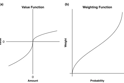
into subjective utilities using a steeper, convex function (see Figure 1.1). The loss
function is convex only because it is upside down. It is still the case that a loss of
£100 vs £200 is a larger difference than £1100 vs £1200. A concave value function is
property here is that the reference point serves the evaluation of prospects as gains
and losses.
PT’s value function nicely describes risk seeking behavior in the loss domain
and risk averse behavior in the gain domain, as we saw in the Asian disease problem.
When the programs are presented using a gain frame, people preferred the program
that saves 200 people for sure over the program that saves 600 people with a 33.33%
chance. If 200 lives saved for sure are evaluated using a concave function, they are
worth more than 600 lives saved maybe. However, when the programs are presented
using a loss frame, people preferred the program, which kills 600 people with a
66.66% chance to the program that kills 400 people for sure. Losing a minimum
number of people is so bad that one is willing to take the risk if one can avoid a loss
[image:23.595.98.497.397.665.2]altogether.
Figure 1.1. Prospect theory’s value and probability weighting functions.
The fact that people’s perspective matters and not final wealth is evident in the
isolation effect: If a person is given $100 and is then asked to choose between 0
0 Amount
V
alue
Value Function (a)
Probability
W
eight
winning another $50 for sure or another $100 with a 50% chance, the person is more
likely to choose the safe option. On the other hand, if a person is given $200 and is
then asked to choose between losing $50 for sure or losing £100 with a 50% chance,
the person is more likely to choose the risky option. If people integrated their initial
gift of $100 into the choice and considered their final wealth, the two choices would
be the same. Gains are treated differently from losses, because “losses loom larger
than gains”. Because the impact of a loss is stronger than the impact of a gain, people
are described to be loss averse; they prefer a sure gain in the light of a possible loss,
even if the expected value is higher than the sure option can offer.
PT without editing rules (“stripped PT” in Birnbaum, 2008) can violate
stochastic dominance. In stripped PT the value of a prospect where one can win £100
with 50% chance and otherwise £100 is smaller than the value of a sure £99. This is
because of probability weighting: The weight for 50% is much smaller than an
objective 50% so that when integrated into the £100 prizes the value adds up to less
than £99. In order to avoid that, Kahneman and Tversky (1979) invented some editing
rules. The prospects are edited through a) combination of probabilities if they are
associated with the same outcome (this would be the case in the above example), b)
separation of outcomes that are riskless, or c) if two prospects share an outcome, they
cancel each other out, d) probabilities and outcomes are simplified by rounding and
finally, e) when an alternative is dominated, it needs to be discarded. PT’s editing
rules become obsolete when probabilities are transformed into cumulative decision
weights, like they are in RDUT (Quiggin, 1982). Tversky and Kahneman (1992)
exchanged their former weighting function and editing rules with a cumulative
probability weighting function and developed a more general model, cumulative
than two non-zero outcomes and in CPT different weights can be assigned to identical
probabilities depending on whether an outcome was perceived as a loss or a gain.
CPT does this by assuming people work with the probability of doing at least as well
as £X instead of the probability of receiving £X–that is cumulative probabilities over
a set of events are psychologically elemental, instead of the probabilities of individual
events. With this new feature CPT is able to explain risk seeking and risk averse
behavior or the four-fold pattern within one person by allowing different weighting
functions for losses and gains (Tversky & Kahneman, 1992). The four-fold pattern
describes risk seeking behavior when dealing with large prizes and small
probabilities, and risk averse behavior when dealing with small prizes and low
probabilities considering low stakes. In the loss domain, the same participant will be
risk seeking when dealing with low stakes and will be risk averse when dealing with
high losses. A person is risk-averse if she chooses the safe option over a risky option
with an equal expected value. A person is risk-seeking if she chooses the relatively
risky option under the same circumstances. If the same person chooses between a safe
and a risky option in the loss domain and is risk-seeking and then is asked to choose
between a safe and a risky option and plays for the same amount of money in the gain
domain and is risk-averse, the person displays the reflection effect.
A little after PT was proposed, Loomes and Sudgen (1982) developed regret
theory to make predictions in line with the Allais paradoxes, risk aversion and loss
aversion. In regret theory, there is a number of states of the world, which each occur
with an objective probability that is known to the chooser, or stands for the chooser’s
belief about the occurrence of each possible state. Given one action, there is one
consequence for each state of the world. One assumption that Loomes and Sudgen
expected utility. The choiceless utility function assigns a utility to a consequence that
the chooser has not chosen herself. The consequence is either inflicted or awarded by
somebody else. The utility of choosing an option A, given a particular state of the
world, will be the sum of its choiceless utility and the difference between the joy of
choosing A and not B, and the regret of choosing A and not B, all assuming the same
state of the world, and considering that regret is convex in outcome difference. This
means that large differences in outcomes in transformed into huge amounts of regret.
Taken together, this means that the evaluation of option A is affected by the presence
of option B. Thus, the evaluation is based on the comparison between the options
available, given a specific state of the world.
Note that the (C)PT and regret explanations of the common ratio effect are
quite different. (C)PT explains the common ratio effect by means of an inverse
S-shaped probability weighting function. In contrast to that, regret theory predicts this
effect by assuming that there is disproportionately more regret if the difference
between what is and what might have been is large, as opposed to if the difference
between what is and what might have been is small. In the scaled up version of the
common ratio effect, the largest possible regret is caused when you choose B and get
£0, when choosing A would have delivered a sure £3,000. But in the scaled down
version, it is possible to choose C and receive £0 when choosing D could have offered
£4,000. This difference is larger, and because of the convexity of the regret function,
the anticipated regret of missing out on £4000 dominates the decision. In summary,
scaling down the problems introduces new and particularly regretful comparisons
which reverse the preference. In this framework, anticipated regret is also the main
driver for the reflection effect: The relatively safe option as compared to a riskier
possible gain can lead to regret, which the decision maker wants to avoid, whereas the
relatively risky option is more appealing in the loss domain, because of the higher
possibility to avoid a loss.
The models presented so far are all based on the standard normative models
that were later modified to account for empirical data. (C)PT and regret theory used
psychological insight to adapt EUT. Other modifications like RDUT only aimed at
explaining empirical phenomena and were not concerned with the influence of the
human factor in building their models. There is another class of descriptive models,
which approaches the paradoxes and the choice reversals from a psychological
perspective. In these configural weight models, the weight of an outcome in one
prospect depends on other outcomes in the same prospect. Configural weight models
are somewhat similar to rank-dependent utility models (Birnbaum & Navarette,
1998), but also share similarities with rank-dependent weighting models like CPT. In
configural weight models utilities of options are assumed to be weighted averages of
all possible outcomes per option. The weights depend not only on the outcomes
themselves, but also on the ranks, the probabilities of those outcomes and the point of
view of the judge, e.g., if the judge is a buyer or a seller, or how risk-averse the
person is. TAX, the “transfer of attention and exchange” model (Birnbaum &
McIntosh, 1996; Birnbaum & Stegner, 1979), is a special case of one of these models,
which predicts the paradoxes described above, the preference reversals and the
four-fold pattern. (In addition, TAX predicts many additional phenomena that CPT cannot
account for, see Birnbaum 2008 for a review.) In TAX, a weight is the attention a
decision maker pays to each outcome. An outcome that is more probable should also
get more attention, but depending on somebody’s risk attitudes, the attention gets
50/50 chance for £100 otherwise £0, or £50 for sure. We know people will tend to be
risk averse, and select the sure £50. In EU and prospect theory this risk averse
behavior is explained using a concave utility function where the utility of £50 is more
than the average of the utilities of £0 and £100. But in TAX, attention moves from the
£100 outcome to the £0 outcome, and this movement of attention from the higher to
the lower outcome reduces the attention weighted sum of the values, making this
option less appealing. The same logic is used to explain why people behave as if they
are loss averse: If people are unwilling to accept a bet where they could either win
£200 or lose £200, one only has to assume that people place more attention to “lose
£200” than to “win £200” to give this bet a net negative evaluation and reject it. It is
not necessary to transform money into utility and have losses loom larger than gains,
but just to assume that it is the transfer of attention–weighting–from the better
outcomes to the worse outcomes–that causes risk-averse or loss-averse behavior
(Birnbaum & Navarette, 1998; Birnbaum, 2008). Transfer of attention is also how
TAX predicts the common ratio effect: When choosing between a safe gamble
without the possibility of a £0 outcome, and a relatively risky gamble with the
possibility of a £0 outcome, the weight within the risky gamble shifts from the
possible amount of £4000 to £0, making the riskier gamble less attractive than the
safe gamble with the £3000 win and prompting more risk averse choices. When
choosing between two risky options that both involve the possibility of a £0 outcome,
and evaluating each option separately within one option, attention is transferred from
a possible gain to £0. Now that both options have a drawback, the riskier option
becomes more appealing because it offers a higher win, prompting more risk-seeking
There are several studies demonstrating inconsistencies with neoclassical
rank-dependent theories–CPT is among those theories– that simple configural weight
models can account for (see Birnbaum, 2004, and Birnbaum, 2008 for the most recent
paradoxes). Gain-loss separability, which empirically is found to be violated, but is
predicted by the neoclassical theories, is one of these examples. Wu and Markle
(2008) asked participants to choose between gamble A+ and gamble B+ in the gain
domain and gamble A- and gamble B- in the loss domain. They found that although a
majority of people preferred gamble B+ to A+ and gamble B- to A-, when gamble A+
was mixed with and gamble B+ was mixed with B-, people suddenly preferred
A-mixed to B-A-mixed–that is in the gain domain participants preferred Option B+ when
choosing between
Option A+: win £2000 with a 25% chance or win £800 with another 25% chance and
otherwise nothing, or
Option B+: win £1600 with a 25% chance or win £1200 with another 25% chance and
otherwise nothing.
They also prefer B- when choosing between
Option A-: lose £800 with a 25% chance or lose £1000 with a 25% chance and
otherwise nothing, or
Option B-: lose £200 with a 25% chance or lose £1600 with a 25% chance and
otherwise nothing.
Expectedly, people are risk averse in the gain domain and risk seeking in the
loss domain. However, if the gain gambles are combined with the loss gambles,
people suddenly reverse their previous preferences by choosing option A out of
Option A: win £2000 with a 25% chance or win £800 with another 25% chance, or
and
Option B: win £1600 with a 25% chance or win £1200 with another 25% chance or
lose £200 with a 25% chance or lose £1600 with a 25% chance (see what gambles
Option A and B are composed of in Table 1.2).
By preferring B+ and B-, but also A, people violate gain-loss separability (see
also Birnbaum & Bahra, 2007). Thus, whilst neoclassical theories qualify to explain
findings in single-domain gambles, they fail in mixed gambles. At the same time,
other models–like TAX–can predict and can account for the violation of gain-loss
separability or stochastic dominance (see Birnbaum, 2008). If we judge theories of
choice against empirical evidence and we find that some very prominent theories–in
economics and psychology–can be refuted based not only on violations of normative
principles, but also on assumptions made that are not compatible with people’s
choices, should we still use those models in appropriate contexts?
Table 1.2
Options A and B result from merging Option A+ with A- and Option B+ with B-
respectively. The probabilities to win or lose are 25%. In the one-domain options, the
gambles offer a 50% chance of nothing.
Option A Nonzero Option A+ gains Nonzero Option A- losses
+ £2000 + £800 – £800 – £1000
Option B Nonzero Option B+ gains Nonzero Option B- losses
+ £1600 + £1200 – £200 – £1600
Up to this point the presented models were silent about the information
integration and the choice process at hand when faced with a decision problem. There
is another class of models, which does propose a specific cognitive process for
(1955) proposed that people do not or cannot optimize, but use simple choice rules–
heuristics–to make decisions; because there are constraints to human cognition, which
make it difficult to adhere to normative principles. To reduce the requirements for the
decision maker, the main feature of the proposed heuristics is the neglect or disregard
of some information. The heuristics differ in terms of which information is ignored.
Several researchers argued that by ignoring information when making a decision,
people are able to make even better, or more robust decisions than if they took all
available information into account (Gigerenzer & Todd, 1999).
The decision making literature has benefitted from the formulation of process
models. Already back in the 70s researchers have encouraged process-oriented
models (Payne, 1976; Payne, Bettman, & Johnson, 1993). They argued that collecting
process data will guide us to more accurate models of choice and will help make
much quicker progress in this endeavor (Johnson, Schulte-Mecklenbeck, and
Willemsen, 2008). The priority heuristic (Brandstätter, Gigerenzer, & Hertwig, 2006)
will represent this class here, although as process model as well as descriptive model
it has been convincingly refuted (see Birnbaum, 2010, or Reiger & Wang, 2008, and
also other references below).
Heuristics are process models: they describe step-by-step how people
supposedly make decisions and are perceived as decision making tools, where each
heuristic can be selected depending on the choice problem and where different people
might choose different heuristics for one and the same task. For tasks involving
choices between two options, there are two classes of heuristics that could be
considered: Tallying and lexicographic heuristics. Tallying works by looking through
all attributes of both options in any order and whichever option has more satisfying
options are first ranked and whichever option has the highest value on the most
important attribute, gets chosen (Tversky 1969).
To account for some of the above mentioned violations of EU theory, like the
Allais paradox, the reflection effect, the fourfold pattern or intransitive choice
preferences, Brandstätter, Gigerenzer, and Hertwig (2006) have proposed the priority
heuristic (PH). Using PH, people consider the attributes of a gamble in the following
order: minimum gain, the probability of the minimum gain and lastly the maximum
gain. When the minimum gains differ by at least 10% of the maximum gain, people
stop the evaluation process and choose the option with the higher minimum gain. If
the minimum gains are too similar, then people compare the corresponding
probabilities and choose the gamble with the higher probability of the minimum gain,
if it exceeds the other by 10%. If this too is not the case, they choose the gamble with
the higher maximum gain. The heuristic works the same way for the loss domain,
where the gamble with the lower losses and higher probability of the minimum losses
are chosen.
To predict the fourfold pattern, consider the following two options. Option A
offers a 95% chance of £100 otherwise nothing and option B offers £95 for sure. First,
the minimum gains are compared; £0 from option A and £95 from option B. £95 (the
higher minimum gain) is higher than 10% of £100 (the maximum gain) so that now
according to the heuristic, people would choose the sure option B, displaying risk
aversion. The priority heuristic would explain risk seeking choices in the exact same
way if the above gambles would involve losses. This is also how the common ratio
effect works in PH: When choosing between two gambles,
Option A: 80% chance of winning £4000, otherwise nothing,
Option B: 100% chance of winning £3000,
PH predicts that people choose the safe gamble B, because the minimum gain of B
(£3000) is by more than 10% of the maximum gain (10% of £4000 = £400) higher
than £0. If these gambles are transformed into
Option C: 20% chance of winning £4000, otherwise nothing,
or
Option D: 25% chance of winning £3000, otherwise nothing,
PH predicts that people choose the riskier option C. Because the minimum gains are
£0 in both options, and the probabilities of the minimum gains do not differ by at least
10%, the option with the higher maximum gain will be chosen.
The priority heuristic has been criticized on several levels. There are several
studies showing that people do not deal with one cue at a time (Birnbaum, 2008;
Hilbig, 2008), that choice patterns and reaction times are more supportive of
strategies that integrate probabilities with outcomes (Ayal & Hochman, 2009;
Glöckner & Betsch, 2008), and that probabilities, which are ignored by PH
systematically influence people’s choices (Fiedler, 2010). Birnbaum (2008) also
showed that PH failed to perform on a significant proportion of the paradoxes that he
himself brought forward and was always outperformed by TAX. Hilbig (2010)
pointed to a general problem considering the validity of heuristics: Even if the
predictions of the simple choice strategies come true, it does not mean that those were
the rules that participants used to make the decision with. Johnson,
Schulte-Mecklenbeck, and Willemsen, (2008) take the same line and strongly argue for the
collection of process data when investigating process models; it is the only way to
participants approach the choice problems varies across individuals and across the
different types of gambles and cannot easily be built into the PH.
The first models I presented are built on normative principles. In their
development, those principles have been relaxed to account for more empirical data
whilst abiding to as many normative rules as possible and dropping as many as
necessary; all in the economic tradition. The TAX model, while not defined as a
process model by its author, but as an as-if model, shifts the interpretation of options
away from being perceived as prospects to trees with branches and proposes that the
shift of attention to different possible outcomes is what leads to violations of
normative principles and the observed choice behavior. What TAX has in common
with the earlier models like PT, regret theory, and EU is the assumption that amounts
are transformed into utility, or value by stable and well-defined functions. However,
there is an increasing range of research (including the experiments presented later on)
challenging this assumption of the stability of value functions. These challenges are at
least partly met by decision by sampling (DbS, Stewart, Chater, & Brown, 2006), a
process model based on simple psychological principles that combined lead to a
context-dependent evaluation of options.
The formulation and integration of the information process during choice often
resembles a normative economic account rather than a model based on psychological
principles. Models within psychology itself (although not in the adaptive decision
maker literature) often even assume that value is computed (Vlaev, Chater, Stewart, &
Brown, 2011), for example by multiplicative integration of transformed attributes.
Those transformations can depend on other available attributes in the option (like in
Opposed to this account, in other models, attributes are evaluated relative to
other attributes so that the value of an option stands in relation to other available
options in the choice set. In this account, value is not computed by using an internal
map that transforms probabilities into weights and amounts into subjective value.
Instead, comparisons between alternatives contribute to the evidence for one
alternative over the other, so that the value of an option on its own is not ever even
calculated or used at any point during a choice (Vlaev, Chater, Stewart, & Brown,
2011).
In these models value is dependent on the comparison process, either with the
immediate context or with attributes from long-term memory. All experiments
presented in this thesis are constructed to test whether, when, and to what degree
comparison processes influence choices between two gambles, ratings of gambles or
simply monetary outcomes. Our hypotheses are based on predictions from decision by
sampling (DbS, Stewart, Chater, & Brown, 2006). In DbS, the rank order of an
attribute value within a decision sample, determines the subjective value of an option,
without people ever calculating or constructing the subjective value of an option.
Instead, DbS is formulated as a process model, where in order to evaluate an option,
people compare it with other options on offer and keep track of the number of times
the current option has won across a series of pairwise comparisons. Thereby people
behave as if they use the subjective value when they make a decision. For example, in
a sample of £3, £5, £6, £10, £13, the subjective value of £13 is higher than in the set
of £6, £13, £16, £19, £23, because £13 wins all binary comparisons in the first set and
receives the value 1, whereas it only wins one comparison out of four possible
comparisons in the second set and receives the value 1/4 there. The higher the
chosen among other available options. The rank hypothesis suggests that the
subjective value of any given option is determined by the distribution of outcomes
available in the choice set and/or in long-term memory.
Stewart, Chater, and Brown (2006) have shown that assuming pairwise
comparisons, frequency accumulation, and sampling from memory, combined with
the distributions of credits and debits in the world, is all you need to produce the
shape of a typical psychoeconomic function–concave value function for credits,
convex value function for debits. The real world distributions of amounts serve as
approximation of what amounts are in people’s long-term memory. That is, to the
extent that memory is adapted to and reflects the structure of the environment
(Anderson & Schooler, 1991), properties of the distributions of attribute values in the
environment could be a useful proxy for the properties of the distributions of attribute
values in people’s memories. What Stewart et al. found in credits and debits to and
from bank accounts, which they used as a proxy for the distributions of gains and
losses in people’s memories, is that there are more small than large credits (i.e., a
positively skewed distribution), and more small than large debits. The positively
skewed distributions mean that for a fixed size increase, the effect will be larger if the
increase is lower in the distribution than if it is higher in the distribution. For example,
because there are more small gains than large gains, an increase of £100 from £0 to
£100 overtakes more of the sample than an increase of £100 from £1000 to £1100.
This is because there are many gains that lie in between $0 and £100, but few gains
lie in between £1000 and £1100. The positively skewed distribution of gains in the
real world combined with the decision-by-sampling principles gives a reasonable
account for the diminishing marginal utility that is assumed in neoclassical theory and
Recently, Stewart, Reimers, and Harris (2015) have experimentally tested the
following DbS prediction: when participants encounter attribute values (e.g., amounts,
probabilities or times) that are positively skewed, with many smaller attribute values
at the low end of the range, the estimated psychoeconomic functions should come out
more concave than when participants encounter attribute values that are negatively
skewed, with many larger attribute values at the high end of the range. The
psychoeconomic functions should also come out more concave than when attribute
values are uniformly distributed. According to the rank principle, the utility of an
attribute increases quickest where the distribution is densest. Finding the predicted
functional forms, means that just by changing what distributions of attributes people
have to deal with, is what will make them prefer more or less risky options. The
authors asked participants to choose between pairs of gambles, whose outcome
distributions were either positively skewed or the participants chose between pairs,
whose outcome distribution was negatively skewed. As predicted, the recovered
utility functions had a concave form when the distribution of outcomes was positively
skewed, whereas it was convex when the distribution of outcomes was negatively
skewed. This means that the subjective value of a presented attribute was higher when
it was presented among a positively skewed distribution where it occupied a relatively
high rank position than when it was presented among a negatively skewed distribution
where it occupied a relatively lower rank position. The analogous procedure was
performed for probabilities and also times separately, reaching the same conclusion.
This means that people might not be inherently risk averse or loss averse, but
that they just appear as if they were, because of the world we live in. With this logic,
because of the way losses and gains are distributed in the real world, people behave as
[image:38.595.96.509.131.366.2]if they were loss averse and only therefore displayed loss aversion?
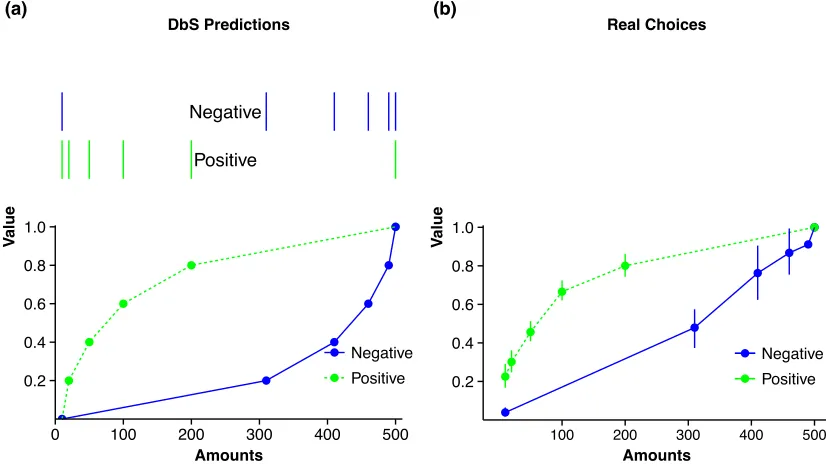
Figure 1.2. Figure 1.2(a) shows the predictions given participants experience the
negative or the positive condition. The top part represents the distribution of amounts
in the two conditions of the experiment. Figure 1.2(b) shows estimated value
functions from real choices under the according conditions.
To test this hypothesis, Walasek and Stewart manipulated the range of
possible gains and losses to spread from $20 loss to a $20 gain (or $40 loss to $40
gain), a $20 loss to a $40 gain or a $40 loss to a $20 gain. They then asked
participants to accept or reject different offers composed of losses and gains, like a
50% probability to lose $10 and 50% to win $10. What does the range of losses and
gains mean for the ranks of the amounts in the respective categories? If the gain-loss
ranges are symmetrical, $10 has the same rank among losses than it has among gains.
Because the evaluation is predicted to be rank-dependent, participants should equally
likely accept or reject a gamble offering to equally likely win or lose $10. If losses
reach up to $20 and gains up to $40, then $10 has a higher rank among losses than
Positive Negative 0.2 0.4 0.6 0.8 1.0
0 100 200 300 400 500
Amounts V alue Negative Positive DbS Predictions (a) 0.2 0.4 0.6 0.8 1.0
100 200 300 400 500
among gains. This means that participants should reject this gamble, because a
high-ranking loss cannot be compensated for by a lower-high-ranking gain. The reverse is true
for the condition where losses range up to $40 and gains only up to $20. Now, $10
ranks higher among gains than among losses. The gamble should be attractive,
because the gain has a higher probability of favorable comparisons with the other
gains than the loss has of favorable comparisons with the other losses. The authors
found the predicted pattern: They demonstrated that just by manipulating the range of
available outcomes, participants chose as if they were loss-neutral in the
symmetrically distributed cases, loss-averse when the range of gains was larger than
the range of losses, and even the opposite of loss-aversion in the reverse case.
Both these sets of experiments show a serious departure from and present a big
challenge to accounts of decision making and judgment that assume an inherently
stable mapping between objective values into their subjective equivalents. The
formulation of models that allow for experiments considering different components of
the decision making process will help in identifying the main drivers of valuation. In
this thesis, we test ideas that all assume comparison processes as key to judgment and
choice. All experiments presented are inspired by the finding that context strongly
influences what we choose and like. As many of these findings can be accounted for
by DbS, we use this model to identify potential mechanisms leading to the above
mentioned contextual effects. This thesis comprises of five chapters, in which we test
different aspects of the decision by sampling model using experiments, cognitive
modeling and meta-analyses of our findings.
Chapter 2 and 3 are based on the findings from Stewart, Reimers, and Harris
(2015). The aim was to test how reliable the rank effects mirrored by the difference in
attributable to DbS proposed mechanisms. We used different within-subjects designs
to measure differences in psychoeconomic functions: In a first step, we flagged
gamble pairs, so that they belong either to a positively or negatively skewed
distribution, to assess whether people can keep track of different samples of attribute
values (as they are assumed to keep track of gains and losses separately). We then
retrospectively divided the choices according to their flags and estimated the
differences between the psychoeconomic function for the two different distributions
of attributes. If participants do separate choice pairs according to their flags into
different samples (just as assumed in Walasek and Stewart (2015), where gains are
compared to other gains and losses to other losses), differences in psychoeconomic
functions should resemble those estimated with a between-subjects design. In a
second step, we unflagged those pairs and again retrospectively estimated those
differences between psychoeconomic functions to check if the observed differences
are indeed attributable to DbS-type processes. In Chapter 3, we investigated the role
of working memory by using cognitive load manipulations, where participants made
some choices under high cognitive load or no/low cognitive load, and again estimated
the differences between psychoeconomic functions. If participants’ preferences are
formed via pairwise comparisons of attributes from memory and DbS is correct in
asserting a role for working memory in making a series of binary ordinal
comparisons, we should see a change in people’s choices when working memory is
loaded. In Chapter 4, we first reviewed the literature showing rank effects in risky
choice and then present yet unpublished data by Stewart and Reimers (2008), where
we estimated and compared effect sizes of attribute distributions on choice reversals
and attractiveness ratings of gambles, which are also predicted by DbS. The
Here we moved from choice to valuation and were interested whether positive affect
after winning a prize in light of a salient alternative and other foregone prizes would
have an impact on positive affect ratings, yielding a comparable effect as in Chapter
4. Finally, in Chapter 6 we examined potential causes for the mutable-zero effect,
which describes the phenomenon that an option is favored when it is described with a
“pay zero” attribute instead of a “receive zero” attribute. We investigated how
different salient attribute values and counterfactuals triggered by the words “pay” and
“receive” could lead to such context effects, prompting choice reversals. Chapter 7
2 Examining how utility and weighting functions get their shapes:
A multi-level, quasi-adversarial, replication
Recently, Stewart, Reimers and Harris (2015, SRH hereafter) presented evidence
from a series of experiments putatively demonstrating that the utility and probability
weighting functions revealed by fitting standard economic models to binary choice
data were sensitive to changes in the distributions of payoffs and probabilities in the
choice sets. While for some the existence of such sensitivity may be no surprise (e.g.
Drichoutis and Nayga, 2013; Etchart-Vincent, 2004; Fehr-Duda et al. 2010, 2011), the
extent of malleability identified by SRH is considerable. For example, for some
distributions of probabilities and payoffs, SRH were able to produce concave utility
functions and inverse-S shaped probability weighting functions as commonly reported
elsewhere in the literature; yet, for other distributions they were able to generate the
mirror image patterns (i.e., convex utility and S-shaped probability weighting
functions). As a convenient label, we will refer to the apparent malleability of the
utility and probability weighting functions identified by SRH as the SRH effect.
At face value, the SRH effect poses a severe challenge to any model of risky
decision making in the preference-theoretic tradition which, thereby, seeks
explanations of choice grounded on the presumption of stable preferences. If a
researcher can, as SRH explicitly suggest, choose the shapes of the functions they
wish to reveal by adjusting the set of gambles used to elicit them, then the
interpretation that such procedures reveal underlying preferences is undermined and
central premises of welfare economics should be reconsidered. Hence, the SRH effect
provides powerful new ammunition for those critical of the adequacy of
preference-based models of risky-choice (Friedman et al. 2014, Gigerenzer, 2016). By contrast,
particular, it provides support for the model of Decision by Sampling (Stewart, 2009;
Stewart et al. 2006), because predictions of this model (which we refer to as DbS for
short) prompted discovery of the SRH effect.
But before interpreting the SRH effect as a strong challenge to preference
based models (or support for procedural models including DbS), it is appropriate to
question whether the effect is replicable and robust. That question is pertinent, not
least, in the light of contemporary controversy surrounding the replicability of many
of the findings in the behavioral sciences and elsewhere (e.g., Camerer et al. 2016;
Maniadis et al. 2014; Open Science Collaboration, 2015). Given this background
controversy and the challenging nature of the SRH findings, we believe good
scientific practice demands careful scrutiny of the SRH effect, via attempts at
replication, to properly assess its significance. With this motivation in mind, this
paper reports an extensive set of replication experiments investigating two primary
issues: first, we examine whether the SRH effect is replicable and robust to variations
in experimental design; second, since we do find support for the SRH effect, we also
probe its origins.
In what follows, we report a set of 14 new experiments conducted as part of
what we call a quasi-adversarial collaboration, and combine these with a reanalysis
of the fixed original experiments. The term “adversarial collaboration” has been used
to refer to experimental research projects jointly planned and executed by two or more
researchers (or research groups) who have ex-ante conflicting hypotheses about its
outcome (for discussion and examples see Bateman et al. 2005; Corrigan, 2011;
Kahneman, 2003; Latham et al. 1988; Mellers et al. 2001). While our collaboration
does not have exactly this form (hence the qualifier ‘quasi’), the seven researchers
psychology), different labs, and have very different degrees of prior investment in the
competing theoretical frameworks that would be supported or challenged by the
existence of the SRH effect. We also use the qualifier “quasi’ to signal that the set of
experiments reported here did not emerge from a common plan of adversarial
collaboration agreed before any of the experiments began. Instead, our collaboration
emerged as subsets of the present co-authors began to discover that we were
undertaking very closely related work exploring the SRH effect, independently, at
different labs. We then began to compare results and, later, discuss designs for new
experiments. Further experiments were subsequently run by different sub-groups of
us, based in three different labs at two universities, using a mixture of lab-based and
online protocols. The development of the designs involved varying degrees of
consultation between us, as well as key variations in designs and procedures, which
we document below. Through this process we have generated a rich source of
evidence relative to the SRH effect, which we bring together in this paper.
The somewhat organic evolution of the collaboration does not mean that the
set of replications, when viewed as a whole, lack structure. We will argue that,
although we did not set out with this explicit purpose, the resultant set of experiments
reflect and, indeed, extend a replication strategy proposed by Levitt and List (2009).
They advocate a methodology involving replication at three levels: reanalysing data
from the original study to be replicated; running fresh experiments using designs
approximating the experiment to be replicated and thirdly, conditional on replicating
the original results, running experiments to probe origins of the phenomenon
observed. Our experiments involve replication at all three levels but we also add a
further dimension to our analysis. Through our experiments, we generated a rich data
complements the individual experiments by placing confidence bounds on the size of
the SRH effect and allowing assessment of how it varies with some key design
features of our replications. As such we interpret part of our contribution as piloting
an extended, four level, version of the Levitt and List (2009) methodology enhanced
via a meta-analysis.
We reach two main conclusions. First, based on replication Levels 1 and 2, we
conclude that the SRH effect is replicable, robust and the meta-analysis (Level 4)
confirms a non-zero effect size. Hence, we reconfirm the challenge posed by SRH to
those who seek to understand choice through the lens of standard preference based
models. Second, based on the Level 3 analysis, we cast doubt on DbS as an account
of the SRH effect since this model at best explains only about half of the effect size
observed in our analysis. Hence, we identify the need for further investigation to
explain the causes of the SRH effect that we observe in our data.
The paper is organized as follows. We first review key features of the original
SRH study and its basic findings. We then summarize the analysis of our results from
all four levels of the replication process. Next we discuss our main findings, and the
last section concludes.
SRH’s (2015) study: setup, motivation, methodology and results
The main results in the SRH original study are based on data generated from
experiments in which individuals had to make a series of choices between pairs of
gambles of the form “p chance of x, otherwise nothing” or “q chance of y, otherwise