University of Warwick institutional repository:http://go.warwick.ac.uk/wrap
A Thesis Submitted for the Degree of PhD at the University of Warwick
http://go.warwick.ac.uk/wrap/71098
This thesis is made available online and is protected by original copyright. Please scroll down to view the document itself.
Bubble Dynamics under Dual
Submitted to the University of Warwick
Doctor of Philosophy
Bubble Dynamics under Dual-Frequency Acoustic
Excitation
by
Yuning Zhang
Thesis
Submitted to the University of Warwick
for the degree of
Doctor of Philosophy
School of Engineering
April 2015
Contents
Contents... i
List of Tables... vi
List of Figures ...vii
Acknowledgements... xvi
Declarations ...xvii
List of Publications...xviii
Nomenclature... xix
Roman letters (alphabetical order)... xix
Greek Letters (alphabetical order) ...xxii
Abstract ... xxiv
Chapter 1 Introduction ... 1
1.1 Research background ... 1
1.1.1 Sonoluminescence under multi-frequency excitation ... 2
1.1.2 Sonochemistry... 5
1.1.3 Biomedical applications ... 7
1.2.1 Dissociation Hypothesis ... 8
1.2.2 Nucleation ... 9
1.2.3 Other mechanisms ... 12
1.3 Bubble dynamics under acoustic excitation... 13
1.3.1 Oscillations of bubbles ... 13
1.3.2 Acoustical scattering cross section... 20
1.3.3 Bjerknes forces ... 22
1.3.4 Bifurcation and Chaotic oscillations ... 25
1.4 Objectives of thesis ... 30
Chapter 2 Fundamentals of Bubble Dynamics under Dual-Frequency Excitation ... 33
2.1 Basic equations and solutions... 34
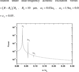
2.2 Response of bubbles under dual-frequency acoustic excitation 37 2.2.1 Basic structures ... 37
2.2.2 Combination resonances ... 45
2.2.3 Simultaneous resonances... 51
2.3.1 Influence of the amplitude of sound pressure and the bubble
size... 53
2.3.2 Influence of the energy allocation between two component sound waves ... 57
2.3.3 Influence of phase difference ... 63
2.3.4 Influence of driving frequency... 64
2.4 Summary ... 66
Chapter 3 Acoustical Scattering Cross Section of Gas Bubbles under Dual-Frequency Acoustic Excitation ... 69
3.1 Basic equations ... 70
3.2 Solutions ... 72
3.2.1 Analytical solution ... 72
3.2.2 Numerical simulations... 74
3.3 Comparisons between analytical solution and numerical simulations ... 78
3.4 Nonlinear characteristics of the scattering cross section under dual-frequency acoustic excitation ... 82
3.5 Influential parameters on scattering cross section... 86
Chapter 4 The Secondary Bjerknes Force under Dual-Frequency
Excitation ... 94
4.1 Equations and solutions ... 95
4.1.1 Basic equations... 95
4.1.2 Analytical solutions... 97
4.1.3 Numerical simulations... 101
4.2 Comparison between the analytical solution and the numerical simulations ... 103
4.3 The basic features of the secondary Bjerknes force under dual-frequency excitation ... 107
4.4 Influence of the pressure amplitude ... 116
4.5 Summary ... 126
Chapter 5 Conclusions ... 128
5.1 Achievements ... 128
5.2 Future work ... 130
Appendix A: Constants used for calculations... 134
Appendix C: Mass Transfer across Interfaces of Gas Bubbles under
Dual-Frequency Acoustic Excitation ... 150
List of Tables
Table 2.1 The categories of the bands in Figure 2.4 and their power. 42
Table 2.2 The power of the bands in Figure 2.4, as a function ofn,m and
n m . 44
Table 2.3 The power of bands (1,0) and (1,1) for different cases shown in
Figure 2.6. 46
Table C1 Bubble growth regions under single-frequency excitation and
dual-frequency excitation with different N. Pe 60000 Pa, 45000 Pa and
List of Figures
Figure 1.1 A brief demonstration of bubbles under multi-frequency
acoustic excitation. 2
Figure 1.2 Time history of the hydrophone output and of the
photomultiplier. 11
Figure 1.3 Time history of the hydrophone output and of the
photomultiplier for different time intervals between low-frequency field
off and high-frequency field on. 11
Figure 1.4 Frequency response curves for a bubble in water with
equilibrium radius of 10 μm for different sound pressure amplitudes. 15
Figure 1.5 Threshold for the occurrence of the first subharmonic
oscillation (of order 1 2 ) versus the equilibrium bubble radius. 16
Figure 1.6 Non-dimensionized bubble radius versus time. 17
Figure 1.7 Power spectrum of the bubble oscillator corresponding to
Figure 1.6. 18
Figure 1.8 Experimental spectrum of the scattered signal from bubbles
excited by a dual-frequency ultrasound field. 19
Figure 1.9 Period-doubling route to chaos via an infinite cascade of
period-doubling bifurcations. 26
pressure amplitude Ps 40 kPa. 27 Figure 1.11 Bifurcation diagrams showing the evolution of the resonance
1,2
R for increasing sound pressure. 28
Figure 2.1 Variations of the non-dimensional bubble radius during its
oscillation under single-frequency acoustic excitation versus time. 38
Figure 2.2 Variations of the non-dimensional bubble radius during its
oscillation under dual-frequency acoustic excitation versus time. 39
Figure 2.3 Power spectrum of bubble oscillations under single-frequency
acoustic excitation. s 0.030. 39
Figure 2.4 Power spectrum of bubble oscillations under dual-frequency
acoustic excitation. 1 0.030. 2 1.91 0.0570. 40
Figure 2.5 The power of various resonances shown in Figure 2.4 plotted
versusnandm. 43
Figure 2.6 Power spectra of bubble oscillations under dual-frequency
acoustic excitation with 10.350 and 2 0.650 , 0.450 ,
0
0.25 , 0.850 respectively. 46
Figure 2.7 Response curves of gas bubble oscillations under the
single-frequency excitation and the dual-frequency excitation.
1 0.35 0
. P Pe 0 0.0707. 49
Figure 2.8 Response curves of gas bubble oscillations under the
1 0.35 0
. P Pe 0 0.424. 50
Figure 2.9 Response curves of bubble oscillation under dual-frequency
excitation when 2 0 0.35 0.65 with: 1 1.40, 1.450, 1.50,
0
1.6 respectively. P Pe 0 0.141. 52 Figure 2.10 Response curves of bubble oscillation under dual-frequency
excitation with different pressure amplitude: 12 0.05, 0.1, 0.2, 0.3.
1 0.35 0
. R0 1 μm. 54 Figure 2.11 Response curves of bubble oscillation under dual-frequency
excitation with different pressure amplitude: 12 0.05, 0.1, 0.2, 0.3.
1 0.35 0
. R0 10 μm. 55 Figure 2.12 Response curves of bubble oscillation under dual-frequency
excitation with different pressure amplitude: 12 0.05, 0.1, 0.2, 0.3.
1 0.35 0
. R0 50 μm. 56 Figure 2.13 Power spectra of bubble oscillations under dual-frequency
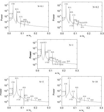
excitation withN= 0.1, 0.2, 1, 5, 10 respectively. 58 Figure 2.14 The response curves of bubble oscillation under
single-frequency and dual-frequency (with N = 0.2, 0.5, 1, 2, 5 respectively) acoustic excitation. 10.350. P Pe 0 0.0707. 60 Figure 2.15 The response curves of bubble oscillation under
Figure 2.16 Amplitude of bubble oscillation versus power allocation at
combination resonances (1,1), (-1,1), (2,1), and (1,2). 62
Figure 2.17 Variations of the non-dimensional bubble radius during its
oscillation under dual-frequency excitation versus time. 2 1= 0,
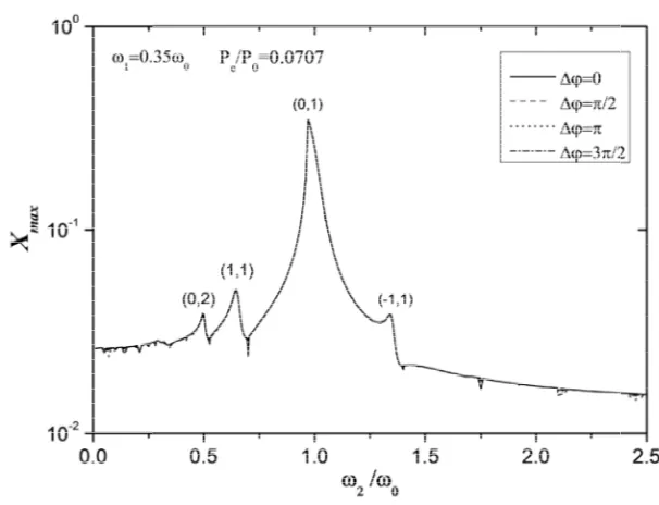
π/2, π, 3π/2 respectively. 63
Figure 2.18 Response curves of bubble oscillations under dual-frequency
excitation with different phase difference: 2 1= 0, π/2, π, 3π/2
respectively. 64
Figure 2.19 Response curves of bubble oscillation under dual-frequency
excitation with different frequencies 1 0.350 , 0.50 , 0.80 ,
0
2.35 . 65
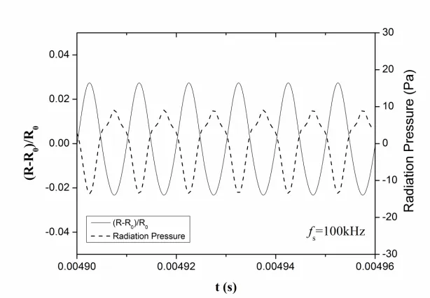
Figure 3.1 The non-dimensional instantaneous bubble radius under the
single-frequency acoustic excitation and corresponding radiation pressure
versus time. 77
Figure 3.2 The non-dimensional instantaneous bubble radius under the
dual-frequency acoustic excitation and corresponding radiation pressure
versus time. 78
Figure 3.3 Predictions of acoustical scattering cross section versus
equilibrium bubble radius under single-frequency acoustic excitation by
analytical solution and numerical method with P Pe 0 =0.01, 0.05, 0.1
Figure 3.4 Predictions of acoustical scattering cross section versus
equilibrium bubble radius under dual-frequency acoustic excitation by
analytical solution and numerical method with P Pe 0 =0.01, 0.05, 0.1
respectively. 81
Figure 3.5 Acoustical scattering cross section versus equilibrium bubble
radius under single-frequency acoustic excitation with P Pe 0=0.1, 0.3, 0.5 and 0.7 respectively. fs 100 kHz. 83 Figure 3.6 Acoustical scattering cross section under single-frequency and
dual-frequency acoustic excitation. f1180 kHz. f2 320 kHz. 0 0.3
e
P P . 85
Figure 3.7 Acoustical scattering cross section versus equilibrium bubble
radius under dual-frequency acoustic excitation with P Pe 0=0.1, 0.2, 0.3 and 0.4 respectively. f1180 kHz. f2 320 kHz. 87 Figure 3.8 The predictions of acoustical scattering cross section under
single-frequency and dual-frequency acoustic excitation withN=0.2, 0.5, 1, 2, 5 respectively. f1180 kHz. f2 320 kHz. 89 Figure 3.9 Acoustical scattering cross section versus equilibrium bubble
radius under dual-frequency acoustic excitation with f1 100 kHz and 2 160
f kHz, 200 kHz, 300 kHz, respectively. 91 Figure 4.1 Predictions of the secondary Bjerknes force coefficient fB
excitation by analytical solution and numerical simulations. fs 100 kHz. R01 10 μm. 104 Figure 4.2 Predictions of the secondary Bjerknes force coefficient fB
versus the equilibrium radius of bubble 2 under dual-frequency excitation
by analytical solution and numerical simulations. f1100 kHz. 2 200
f kHz. R0110 μm. 105 Figure 4.3 The variations of the secondary Bjerknes force coefficient fB
in the R01R02 plane under single-frequency and dual-frequency excitation. P Pe 0 0.03. f1 100 kHz. f2 200 kHz. 110 Figure 4.4 The variations of the secondary Bjerknes force coefficient fB
with the change of equilibrium bubble radius of bubble 2 when the radius
of bubble 1 is fixed as 10 μm, 25 μm, and 40 μm respectively. 112
Figure 4.5 The variations of the secondary Bjerknes force coefficient fB
in the R01R02 plane under single-frequency and dual-frequency excitation. P Pe 0 0.3. f1 100 kHz. f2 150 kHz. 114 Figure 4.6 The variations of the secondary Bjerknes force coefficient fB
in the R01R02 plane under single-frequency and dual-frequency excitation. P Pe 0 0.1. f1 100 kHz. f2 200 kHz. 119 Figure 4.7 The variations of the secondary Bjerknes force coefficient fB
Figure 4.8 The variations of the secondary Bjerknes force coefficient fB
with the sound pressure amplitude under single-frequency and
dual-frequency excitation. 122
Figure 4.9 Normalized driving pressure, the instantaneous bubble radii of
the two bubbles and v v 1 2 versus normalized time under single- and
dual-frequency excitation. 124
Figure 4.10 The instantaneous bubble radii of the two bubbles and v v 1 2
versus normalized time under dual-frequency excitation with P Pe 0=0.03,
0.1, and 0.2 respectively. 125
Figure B1 Frequency response curves predicted by three approaches (a)
“=1.4, th=0”, (b) “=1.0, th=0”, and (c) “Present” for pressure
amplitudes from 0.05 to 1.2. R0 =2 μm. The values of and th employed in the approach “Present” (d). 140
Figure B2 Frequency response curves predicted by three approaches (a)
“=1.4, th=0”, (b) “=1.0, th=0”, and (c) “Present” for pressure
amplitudes from 0.05 to 0.6. R0 =10 μm. The values of and th employed in the approach “Present” (d). 141
Figure B3 Frequency response curves predicted by three approaches (a)
“=1.4, th=0”, (b) “=1.0, th=0”, and (c) “Present” for pressure
Figure B4 Frequency response curves predicted by three approaches: “
=1.4, th=0”, “=1.0, th=0”, and “Present”.R0=2 μm. ε = 1.2. 143
Figure B5 Frequency response curves predicted by three approaches: “
=1.4, th=0”, “=1.0, th=0”, and “Present”.R0=10 μm. ε = 0.6. 143
Figure B6 Frequency response curves predicted by three approaches: “
=1.4, th=0”, “=1.0, th=0”, and “Present”.R0=50 μm. ε = 0.6. 144
Figure B7 Comparisons of the onset curves of subharmonic resonance
with the order of 1
2 predicted by three approaches: “=1.4, th=0”, “
=1.0, th=0”, and “Present”.R0=10 μm. 145
Figure B8 Comparisons of the threshold of subharmonic resonance with
the order of 1
2 predicted by three approaches (“=1.4, th=0”, “=1.0,
th
=0”, and “Present”) versus equilibrium radius of bubbles. 147
Figure C1 The predicted threshold of the total acoustic pressure amplitude
of rectified mass diffusion under single-frequency and dual-frequency
acoustic excitation. 5 1 1 5 10 s
. 6 1
2 3 1 1.5 10 s
. 154
Figure C2 The predicted threshold of the total acoustic pressure amplitude
of rectified mass diffusion under single-frequency and dual-frequency
acoustic excitation with N= 0.2, 0.5, 1, 2, 5 respectively. 5 1 1 5 10 s
.
6 1 2 3 1 1.5 10 s
. 157
Figure C3 The predicted threshold of the total acoustic pressure amplitude
acoustic excitation with N= 0.2, 0.5, 1, 2, 5 respectively. 1 5 105s1. 6 1
2 10 1 5 10 s
. 158
Figure C4 Predicted local maximum threshold pressure under
dual-frequency excitation versus the ratio of two excitation acoustic
pressure amplitudes. 5 1 1 5 10 s
. 2=31, 51, 101 respectively.
Acknowledgements
Firstly, I would like to show my deepest gratitude to Professor Shengcai Li,
who has provided me excellent supervision, academic guidance and
encouragements. I would also like to thank Dr. Duncan Billson for his help
and valuable suggestions on the writing of this thesis. I would also
acknowledge the financial support from China Scholarship Council and
the tuition fee support from the School of Engineering, University of
Warwick.
I would love to show special appreciations to my parents and my husband
for their long-term and unconditional support and encouragements.
Without them, I cannot finish this PhD thesis.
I would also like to thank Mr. Huw Edwards, Dr. Ting Chen and Dr.
Ching-Hsien Chen for their kind help.
Last but not least, I would like to thank all my lovely friends, especially
Xisha Chen, Yaru Chen, Yi Ding, Tianrong Jin, Chunzhi Ju, Xuqin Li,
Huaiju Liu, Lei Wang, Zhongnan Wang, Wei Xing, Min Yang, Jinghan
Declarations
I herewith declare that this thesis contains my own work conducted under
the supervision of Professor Shengcai Li and Dr. Duncan Billson. No part
of the work in this thesis was previously submitted for a degree at another
List of Publications
* indicates the correspondence author
1. Zhang, Yuning* and Shengcai Li. "Acoustical scattering cross section
of gas bubbles under dual-frequency acoustic excitation." Ultrason.
Sonochem. (2015), in press.
2. Zhang, Yuning*, Duncan Billson and Shengcai Li. "Influences of
pressure amplitudes and frequencies of dual-frequency acoustic
excitation on the mass transfer across interfaces of gas bubbles." Int.
Communications in Heat and Mass Transfer (2015), in press.
3. Zhang, Yuning and Shengcai Li*. "Thermal effects on nonlinear
radial oscillations of gas bubbles in liquids under acoustic excitation."
Int. Communications in Heat and Mass Transfer 53 (2014): 43-49.
4. Zhang, Yuning*, Yuning Zhang and Shengcai Li. “Bubble dynamics
under acoustic excitation with multiple frequencies.” Int. Symp.
Cavitation and Multiphase Flow, Oct, 18th-21th, Tsinghua University,
Beijing, China.
5. Zhang, Yuning*, Yuning Zhang, Xiaoze Du, and Haizhen Xian.
"Enhancement of heat and mass transfer by cavitation." Int. Symp.
Cavitation and Multiphase Flow, Oct, 18th-21th, Tsinghua University,
Nomenclature
Roman letters (alphabetical order)
A amplitude of the incident wave
B/r amplitude of the divergent spherical scattered wave l
c speed of sound in the liquid (m/s) 12
e unit vector pointing from bubble one to bubble two s
f frequency of external single-frequency sound field (Hz) 1
f frequency of external sound field of frequency 1 (Hz) 2
f frequency of external sound field of frequency 2 (Hz) B
f the secondary Bjerknes force coefficient B
F the secondary Bjerknes force (N)
L separation distance between the centres of two bubbles (m)
N ratio of the pressure amplitudes of the two component acoustic waves under dual-frequency excitation
0
P ambient pressure (Pa) s
P acoustic pressure amplitude of single-frequency excitation (Pa)
1 A
P pressure amplitude of one of the component acoustic wave of the dual-frequency excitation (Pa)
2 A
wave of the dual-frequency excitation (Pa)
e
P total input power (Pa) rad
P radiation pressure (Pa) 1
rad
P radiation pressure generated by the oscillations of bubble two at the centre of bubble one (Pa)
2 rad
P radiation pressure generated by the oscillations of bubble two at the centre of bubble one (Pa)
1
p
pressure gradient generated by bubble one at the centre of
bubble two
2
p
pressure gradient generated by bubble two at the centre of
bubble one
r radial coordinate from the origin of the centre of the bubble (m)
R instantaneous bubble radius (m)
R1 instantaneous radius of bubble one (m)
R2 instantaneous radius of bubble two (m)
R first derivative of the instantaneous bubble radius (m/s)
R second derivative of the instantaneous bubble radius (m/s2) 0
R equilibrium bubble radius (m) 01
R equilibrium bubble radius of bubble one (m) 02
max
R maximum radius of the bubble during steady-state oscillations (m)
rs
R corresponding resonance bubble radius of the driving frequency of the single-frequency excitation (m)
1 r
R corresponding resonance bubble radius of one component driving frequency of the dual-frequency excitation (m)
2 r
R corresponding resonance bubble radius of the other component driving frequency of the dual-frequency
excitation (m)
t time (s)
T period of bubble oscillation (s) 1
v instantaneous volume of the bubble one (m3) 2
v instantaneous volume of the bubble two (m3)
X non-dimensional instantaneous bubble radius
Greek Letters (alphabetical order)
ac
acoustic damping constant
th
thermal damping constant
tot
total damping constant
vis
viscous damping constant
s
non-dimensional amplitude of single-frequency driving
sound field
1
non-dimensional amplitude of external sound field of
frequency 1
2
non-dimensional amplitude of external sound field of
frequency 2
polytropic exponent
l
wavelength in the liquid (m)
l
viscosity of the liquid (Pa s)
th
effective thermal viscosity (Pa s)
l
density of the liquid (kg/m3)
surface tension coefficient (N/m)
s
acoustical scattering cross section (m2)
s
phase of the acoustic wave of the single-frequency
excitation
1
dual-frequency excitation
2
phase of the other the component acoustic wave of the
dual-frequency excitation
angular frequency of the driving sound field
0
natural frequency of bubble oscillator
s
angular frequency of the driving sound field of
single-frequency
1
one angular frequency of the driving sound field of
dual-frequency
2
another angular frequency of the driving sound field of
Abstract
Acoustic cavitation plays an important role in a broad range of biomedical,
chemical and engineering applications, because of its magnificent
mechanical and chemical effects. Particularly, the irradiation of the
multi-frequency acoustic wave could be favouritely employed to promote
these effects, such as enhancing the intensity of sonoluminescence,
increasing the efficiency of sonochemical reaction, and improving the
accuracy of ultrasound imaging and tissue ablation. Therefore, a thorough
understanding of the bubble dynamics under the multi-frequency acoustic
irradiation is essential for promoting these effects in the practical
applications. The objective of this PhD programme is to investigate the
bubble dynamics under dual-frequency excitation systematically with
respect to bubble oscillations, the acoustical scattering cross section and
the secondary Bjerknes force (a mutual interaction force between two
oscillating bubbles). Spherical gas bubbles in water are considered. Both
analytical analysis based on perturbation method and numerical
simulations have been performed in this thesis.
The analytical solutions of the acoustical scattering cross section and the
obtained and validated. The value of the secondary Bjerknes force can be
considered as the linear combination of the forces derived under the
single-frequency approaches. The predictions of those analytical solutions
will be impaired for the cases with large acoustic pressure amplitudes.
The numerical simulations reveal some unique features of the bubble
dynamics under dual-frequency excitation, e.g., the combination
resonances (i.e., their corresponding frequencies corresponding to the
linear combinations of the two component frequencies) and the
simultaneous resonances (i.e., the simultaneous occurrence of two
resonances in certain conditions). The influence of a number of paramount
parameters (e.g., the pressure amplitude, the equilibrium bubble radii, the
power allocation between the component waves, the phase difference and
the driving frequency) on the bubble dynamics under dual-frequency
excitation is also investigated with demonstrating examples. Based on that,
the parameters for optimizing the dual-frequency approach are proposed.
In addition, the effects of thermal effects and mass transfer on the bubble
dynamics have also been discussed.
Keywords: cavitation, bubble dynamics, dual-frequency excitation,
Chapter 1 Introduction
1.1 Research background
When stimulated by acoustic waves, bubbles in a liquid will oscillate,
termed as “acoustic cavitation” (Plesset and Prosperetti, 1977; Brennen,
1995). Acoustic cavitation has attracted much attention for many years
because of its unique physical complexity (Lauterborn and Kurz, 2010),
chemical applications (Ashokkumar, 2011) and biomedical significance
(Coussios and Roy, 2008). In particular, a considerable body of work has
been produced with multiple-frequency acoustic wave irradiation, i.e., two
or more acoustic waves with the same or different frequencies acting on
the cavitation bubbles simultaneously (as shown in Figure 1.1).
Researchers have found that the use of the multi-frequency ultrasound
field could lower the cavitation thresholds (Ciuti et al., 2000), generate
more new cavitation nuclei (Dezhkunov, 2003), increase the active
cavitational volume (Servant et al., 2003) and improve energy efficiency
(Sivakumar et al., 2002). So multi-frequency approaches have been
Matula, 2000; Holzfuss et al., 1998; Kanthale et al., 2008; Krefting et al.,
2002), to increase the efficiency of sonochemical reactions (Kanthale et al.,
2007; Moholkar, 2009; Brotchie et al., 2007; Feng et al., 2002; Tatake and
Pandit, 2002), to improve the accuracy of ultrasound imaging (Zheng et al.,
2005; Barati et al., 2007; Wyczalkowski and Szeri, 2003) and tissue
ablation (Guo et al., 2013). The efficiency of a wide range of engineering
applications could be significantly promoted by the multiple frequency
ultrasound systems.
Figure 1.1 A brief demonstration of bubbles under multi-frequency
acoustic excitation. This figure was adapted from Fig. 3 of Newhouse and
Shankar (1984).
1.1.1 Sonoluminescence under multi-frequency excitation
ultrasound field, which illustrated the phenomenon of multi-bubble
sonoluminescence (MBSL). Single-bubble sonoluminescence (SBSL) was
firstly fulfiled by Gaitan et al. (1992). The light emitted by the bubble
could even be seen by naked eyes. This emission has been attributed to the
focus of high energy released during bubble collapse (Brenner et al., 2002).
For resent reviews of sonoluminescence, readers are referred to Suslick
and Flannigan (2008), Putterman and Weninger (2000). Many papers have
reported that the use of multi-frequency acoustical excitation is an
efficient way to boost sonoluminescence.
Holzfuss et al. (1998) employed acoustic waves with a combination of the
fundamental frequency and its first harmonic with a wide range of
amplitudes and relative phases to increase the light emission during bubble
oscillations. They reported that the addition of the acoustic wave with the
frequency corresponding to the first harmonic can increase the emission of
sonoluminescence up to 300%, compared with that emitted by the system
with the fundamental frequency alone. It was also found that the relative
phase between the two acoustic components plays an important role on the
intensity of sonoluminescence. The position of the sonoluminescence
bubble was also numerically predicted based on the calculation of the
with experimental data.
Krefting et al. (2002) investigated the influential parameters on the SBSL
under dual-frequency excitation more systematically. They also added the
first harmonic component sound wave into a sinusoidally driven system.
Through experimental measurements and numerical simulations, the
region of light emission was mapped into the parameter space spanned by
the two driving pressure amplitudes and their relative phase. Their results
showed that the addition of the second sound wave is able to amplify
SBSL in particular parameter zones.
Ciuti et al. (2000; 2003) studied the influential factors of the enhancement
of MBSL in acoustic fields with highly different frequencies. In most of
the cases, the addition of a low-frequency acoustic wave into the
high-frequency field lead to stronger light emission, except the case in
which the intensities of both component waves were much higher than the
corresponding cavitation thresholds. For resent researches of
sonoluminescence under multi-frequency excitation, readers are referred
to Hargreaves and Matula (2000), Kanthale et al. (2008), Brotchie et al.
1.1.2 Sonochemistry
The high temperature and pressure created by the bubble collapse can also
promote chemical activities within or near the bubbles, a process termed
as “sonochemistry” (Storey and Szeri, 2000). During such processes, the
formation of free radicals (e.g., OH, H) could induce new reactions or accelerate existing chemical reactions, such as redox process, degradation
of macromolecules and decomposition of organic liquids (Henglein, 1987).
The applications of sonochemistry were reviewed recently in a number of
works (Adewuyi, 2001; Einhorn et al., 1989; Mason, 1999; Nikitenko et
al., 2010).
Like sonoluminescence, the efficiency of sonochemical reactions could be
enhanced by multi-frequency ultrasound approaches. Feng et al. (2002)
employed both continuous and pulsed dual-frequency systems by
combining two ultrasonic transducers: one with frequency of the kilohertz
order and the other one with frequency of the megahertz order. A
three-frequency system was also involved. They detected the release of
iodine, the change of electroconductivity, and the fluorescence formation
under different acoustical excitation conditions. The experiments
illustrated that a combination of the two sound sources can enhance the
further increase the efficiency of sonochemistry. Furthermore, they studied
the influence of the frequency in the low megahertz range. The lower the
frequency was used, the higher cavitation yield was obtained.
The optimization of the cavitation effects in chemical reactors is also an
issue concerned in the applications of sonochemistry. Moholkar et al.
(2000 and 2009) revealed that the mode and spatial distribution of the
cavitation in the reactor could be controlled by adjusting the parameters of
the dual-frequency field. For instance, the phase difference between the
two ultrasound waves has greater influence on the production of radicals
than the frequency ratio does. They demonstrated that it was possible to
overcome the directional sensitivity of the cavitation events and the
erosion of the sonicator surface by adding extra ultrasound waves.
Kanthale et al. (2007) investigated the effects of the intensity and the
frequencies of dual-frequency system numerically and compared the
results with experimental data in the literature. Their work indicated that
there exists an optimum value of the ultrasound intensity in sonochemical
processes. And it is more efficient to use lower operating frequencies.
In the last decade, the application of multi-frequency systems in the field
and Pandit (2002), Servant et al. (2003), Sivakumar et al. (2002), Yasuda
et al. (2007), and Brotchie et al. (2009).
1.1.3 Biomedical applications
Acoustic cavitation has been applied widely in the field of biomedical
engineering. It can enhance the accuracy of ultrasound imaging with the
help of the micro-bubbles (Wu et al., 2003; Barati et al., 2007), promote
drug and gene transfer into tissue and cells (Song et al., 2007; Hernot and
Klibanov, 2008; Newman and Bettinger, 2007), and treat tumours and
ablate tissues (Xu et al., 2004; Maxwell et al., 2011). Multi-frequency
approach can advance these biomedical applications.
He et al. (2006) developed a high intensity focused ultrasound (HIFU)
device which could work both in a single-frequency mode and in a
dual-frequency mode. The experimental results showed that the
dual-frequency HIFU induced larger tissue lesion than under
single-frequency mode within the same time duration, which means that
dual-frequency could improve the efficiency of tumour ablation.
Meanwhile, this improvement also suggests that the main mechanism of
Guo et al. (2013) placed tissues at the focus of HIFU transducers under
single-frequency, dual-frequency and tri-frequency modes respectively.
The multi-frequency mode could yield higher temperatures and a higher
growth rate of the temperature during tissue ablation. Their numerical
simulation agreed well with the experimental results.
1.2 Physical mechanisms
The underlying mechanisms of the effects of multi-frequency acoustical
excitation are still not clear. This section introduces some of the possible
candidates briefly.
1.2.1 Dissociation Hypothesis
Ketterling and Apfel (2000) explained the multi-frequency
sonoluminescence using phase space diagrams based on the dissociation
hypothesis (DH) initially proposed by Lohse and Hilgenfeldt (1997).
Because of the high temperature produced during SBSL, the nitrogen and
oxygen in air bubbles may dissociate to O and N which will compose water soluble chemicals (e.g., NO3 and NH4) in subsequent
reactions (Lohse and Hilgenfeldt, 1997; Lohse et al., 1997). Meanwhile,
waves (Lohse et al., 1997; Hilgenfeldt et al., 1996). Therefore, the mass
transfer through chemical reaction and rectified diffusion should be
considered in SBSL. And the multi-frequency approach could enhance
these effects.
Ketterling and Apfel (2000) constructed a phase diagram based on
calculations of the equations of bubble motion, diffusive equilibrium and
the Mach criterion (assuming that the ratio of the bubble wall velocity and
the speed of the gas is larger than one), which separates the response of the
bubbles into four regions i.e. stable SL, unstable SL, stable non-SL and
unstable non-SL. Comparing their results with the experimental data of
Holzfuss et al. (1998), an excellent quantitative agreement is found.
1.2.2 Nucleation
For multiple bubble cavitation, Cuiti et al. (2000 and 2003) proposed that
when the liquids are irradiated by the ultrasound field consisting of two
highly different frequencies, a large amount of the new nuclei could be
generated by the added low-frequency (LF) acoustic wave, leading to the
enhancement of sonoluminescence.
sonoluminescence intensity did not fall down immediately. On the
contrary, it increased and then decreased smoothly. This phenomenon
suggests that the bubble fragments induced by bubble collapse became
new nuclei with smaller radii than the initial equilibrium radius, which
were likely to collapse in the high-frequency (HF) field. This mechanism
could explain the enhancement of sonoluminescence in the cases of
switching-on the LF and HF fields successively with a certain time
interval (as shown in Figure 1.3). The new nuclei generated by the LF
field could live for at least several seconds so that their oscillation and
collapse could strengthen the intensity of sonoluminescence in the HF
field.
Feng et al. (2002) investigated the cavitation yield from the aspect of
sonochemistry. They also pointed out that the production of new bubbles
by the LF field is one of possible mechanisms for the enhancement of
Figure 1.2 Time history of the hydrophone output (upper record) and of
the photomultiplier (lower record). The black bars above the image
indicate switching-on of the LF field (lower bar) and the HF field (the
higher bar). High-frequency (HF) field parameters: pulse period 100 ms;
pulse duration 2 ms. This figure was adapted from Fig. 3 of Cuiti et al.
(2003).
Figure 1.3 Time history of the hydrophone output (upper record) and of
the photomultiplier (lower record) for different time intervals t
between the LF field off and the HF field on: t 2s(a), 5s (b), 22.5s (c). Other parameters are the same as in Figure 1.2. This figure was adapted
1.2.3 Other mechanisms
1. Periodic decrease in the total quasi-static pressure in the LF field. The LF field is quasi-static in relation to the HF field when the frequency of the LF field is lower (ten times or more) than that of the HF field. The
total pressure (the sum of the hydrostatic pressure and the pressure of the
LF field) decreases during the negative pressure amplitude half-period of
the LF field, leading to the increase of bubble size and bubble quantity. As a result, in the compression half-period, the increase of the LF-field quasi-static pressure may increase the efficiency of the bubble collapse in
the HF-field (Carpendo et al., 1987; Wolfrum et al., 2001; Iernettia et al.,
1997).
2. Suppression of the formation of stable bubble clusters.
The bubbles in clusters are close to each other so that they interact
strongly with shock waves and the Bjerknes forces (Leighton, 1994).
Therefore, bubbles deform under these interactions in the early stage of
collapse. The non-spherical collapse is less efficient from the aspect of the
energy concentration, which is considered to be one of the reasons
decreasing the intensity of MBSL by bubble cluster (Evans, 1996). The
addition of the LF acoustic wave can induce large bubbles. The shock
could prevent the formation of bubble cluster. Hence, the overall
efficiency of the energy concentrated by cavitation bubbles may raise.
3. Optimization of sonochemical reactor.
The modelling and experimental investigation of Tatake and Pandit (2002)
revealed that the introduction of the second sound wave results in better
distribution of the cavitational activity in the reactor, because the
dual-frequency approach uniforms the yields of cavitation, minimises the
formation of standing waves and leads to an effective utilization of the
reactant volume.
1.3 Bubble dynamics under acoustic excitation
In the above sections, one can find that bubble dynamics play an essential
role in the aforementioned cavitation effects and related applications. In
this section, the basic features of bubble oscillations are introduced and
research in the fields of acoustical scattering cross section, the Bjerknes
force and chaos is reviewed.
1.3.1 Oscillations of bubbles
have been developed and reviewed by Plesset and Prosperetti (1977),
Prosperetti (1984a; 1984b), Feng and Leal (1997), Brenner et al. (2002)
and Lauterborn and Kurz (2010).
Lauterborn (1976) gave a thorough investigation of the basic properties of
nonlinear oscillations of gas bubbles in liquids numerically. The response
of a bubble to a single-frequency excitation was calculated and displayed
in the form of frequency response curves, i.e., the maximum bubble radius
in steady-state oscillation (non-dimensionalized by the equilibrium bubble
radius) versus driving frequency. Figure 1.4 shows typical response curves
with special features of nonlinear oscillations. The expression n m (here,
m and n are two integers) above the peaks represents the order of the resonance. Cases with m=1 and n=2, 3… correspond to harmonics; cases withm=2, 3… andn=1 correspond to subharmonics; cases with m=2, 3… and n=2, 3… correspond to ultraharmonics. There exist thresholds for subharmonics and ultraharmonics. Figure 1.5 illustrates the threshold for
the subharmonic of the order 1 2 varying with bubble radii. For detailed
definition and the descriptions of the resonances and nonlinear phenomena
(e.g., jump phenomenon, hysteresis) mentioned above, readers are referred
Figure 1.4 Frequency response curves for a bubble in water with a radius
at rest of Rn 10 μm for different sound pressure amplitudes PA of (a) 0.4, (b) 0.5, (c) 0.6, (d) 0.7, and (e) 0.8 bar. is the frequency of the
driving sound field. 0 is the natural frequency of the bubble oscillation.
max
R is the maximum radius of the bubble during its steady-state oscillation. The numbers marked above the peaks are the orders of the
resonances, represented as n m. The dots and the arrows belong to curve (e). The arrows indicate that the corresponding stationary solution is out of
the range of the diagram or that no stationary solution could be found. In
this case the values of the amplitudes were also very high oscillating
around some value outside the diagram. This figure was adapted from Fig.
Figure 1.5 Threshold for the occurrence of the first subharmonic
oscillation (of order 1 2 at 0 2) versus the equilibrium bubble
radius (solid line). is the frequency of the driving sound field. 0 is
the natural frequency of the bubble oscillation. PA is the amplitude of sound pressure. This figure was adapted from Fig. 13 of Lauterborn
(1976).
The power spectrum can be used to describe the property of bubble
oscillators. By solving the bubble motion equations, the variations of
bubble radius with time could be obtained (as shown in Figure 1.6). Then
through the Fourier transform, the “time domain” diagram could be
transformed to the “frequency domain” diagram, i.e., the power spectrum
[as shown in Figure 1.7(a)], the corresponding frequencies of the bands
resonance and its harmonics. In particular conditions, as shown in Figure
1.7(b), there are bands at 2 , 3 2 and 5 2 which represent
subharmonic and ultraharmonics respectively. These lines are also typical
bands which usually appear in the scattered signals (i.e., acoustical echo of
bubble oscillations) in experiments.
Figure 1.6 Non-dimensionized bubble radius versus time. Equilibrium
bubble radius Rn is 10 μm. Sound pressure amplitude is 90 kPa. Driving
Figure 1.7 Power spectrum of bubble oscillator. Equilibrium bubble radius
n
R is 10 μm. Sound pressure amplitude
207 kHz; (b) 197 kHz.
and Parlitz (1988).
Newhouse and Shanka
oscillators under a dual
1
f and f2 would contain the bands at in single-frequency
the radiated pressure at frequencies
1 2
f f . They (Newhouse and Shankar, 1984; Shanka proved that the resonance at
at f2, which means obtained through dual
(a)
(b)
1.7 Power spectrum of bubble oscillator. Equilibrium bubble radius
ound pressure amplitude is 90 kPa. Driving frequency
kHz. This figure was adapted from Fig. 13 of Lauterborn
Newhouse and Shankar (1984) pointed out that the echo of bubble
a dual-frequency acoustical excitation with frequencies
would contain the bands at f1 f2 besides the typical bands frequency approach. They further gave the analytical solutions of
pressure at frequencies f1, f2 , 2f1, 2f2, f1 f2
They (Newhouse and Shankar, 1984; Shankar et al., 1986) also
the resonance at f1 f2 is much sharper than the resonance , which means more accurate measurements of bubble size can be
dual-frequency approach.
1.7 Power spectrum of bubble oscillator. Equilibrium bubble radius
kPa. Driving frequencyv: (a) This figure was adapted from Fig. 13 of Lauterborn
r (1984) pointed out that the echo of bubble
with frequencies
besides the typical bands
gave the analytical solutions of
1 2
f f , and , 1986) also
the resonance
However, in
multi-bands rather than those corresponding to
driving frequencies. Fig
scattered signal of bubbles ex
frequencies f1 and
corresponding to main resonances (marked by
by □), subharmarnics (marked by
△). But besides these, there are other peaks (marked by
magnitudes of which
Figure 1.8 Experimental spectr
excited by a dual-frequency ultrasound field. The frequencies of the two
sound waves are
1 2 12
f f MHz. of Ma (2010).
-frequency systems, the scattered echo contains
those corresponding to the difference and sum
driving frequencies. Figure 1.8 is an experimental spectrum
scattered signal of bubbles excited by a dual-frequency field (with
and f2 respectively). In this figure, there are peaks corresponding to main resonances (marked by■), their harmonics (marked ), subharmarnics (marked by▲) and sum and difference (marked by
besides these, there are other peaks (marked by
of which are of the same order of the harmonics.
1.8 Experimental spectrum of the scattered signal from bubbles
frequency ultrasound field. The frequencies of the two
sound waves are f15.5 MHz and f2 6.5 MHz, respectively. 2 1 1
f f MHz. This figure was adapted from Fig. contains more
the difference and sum of the
um of the
frequency field (with
In this figure, there are peaks
), their harmonics (marked
sum and difference (marked by
besides these, there are other peaks (marked by ◆), the
of the scattered signal from bubbles
frequency ultrasound field. The frequencies of the two
respectively.
So far as we know, most published papers mainly focused on the
application of the sum and difference of the driving frequencies in
multi-frequency systems (Wyczalkowski and Szeri, 2003; Phelps and
Leighton, 1994; Wu et al., 2005). The fundamental properties of bubble
dynamics (for instance, the special bands marked by ◆ shown in Figure
1.8) under multi-frequency acoustical excitation have not been studied
systematically. However, these features are essential for understanding the
bubble behaviour under multi-frequency excitation as well as expanding
their applications.
1.3.2 Acoustical scattering cross section
During the oscillations of bubbles, a diverging spherical wave can be
emitted and radiation pressure can be generated within the liquid
surrounding the bubbles. The acoustical scattering cross section, defined
as the square of the ratio between the amplitude of the radiated wave by
bubbles and the amplitude of the incident acoustic wave (Medwin, 1977),
is usually employed as a criterion of the scattering ability of the bubbles.
This scattering force of cavitation bubbles is essential for facilitating the
reaction of chemical processes (Shah et al., 1999; Gogate et al., 2001;
Vichare et al., 2000; Yoo and Han, 1982), measuring bubble size
2012), de-agglomerating particle clusters (Wagterveld et al., 2011; Sauter
et al., 2008; Marković et al., 2008), refining grain structures of metals
(Eskin and Eskin, 2003; Eskin, 1994; Komarov et al., 2013), explaining
unusual bubbles in stranding marine mammals caused by anthropogenic
sounds (e.g., sonar) (Jepson et al., 2003; Cox et al., 2006; Crum et al.,
2005), and performing non-invasive therapy and drug delivery (Coussios
et al., 2008; ter Haar and Daniels, 1981; Dollet et al., 2008).
The acoustical scattering cross section of gas bubbles has been studied by
many researchers over several decades. The most widely cited formula for
acoustical scattering cross section of gas bubbles was mainly developed by
Wildt (1946) and Medwin (1977). A near-resonance correction based on
the Wildt-Medwin formula was initially proposed by Weston (1967) and
recently generalized by Zhang (2013a). d’Agostino and Brennen (1988)
studied the acoustical absorption and scattering cross sections of spherical
bubble clouds. Leroy et al. (2009) studied the scattering behaviour of a
monodisperse layer of bubbles. Hilgenfeldt et al. (1998) proposed a
unified theory for the scattering phenomenon of bubbles for diagnostic
ultrasound. Clarke and Leighton (2000) investigated the effects of the
transient state on the scattering cross section of bubbles. However, in the
excitation has not yet been studied.
1.3.3 Bjerknes forces
When gas bubbles are driven by a sound field in a liquid, the radiation
force induced by the acoustic pressure gradient could cause mutual
interaction between bubbles, this phenomenon was firstly reported by
Bjerknes (Bjerknes, 1906). The force due to the direct effect of the sound
field is named as “primary Bjerknes force”. The force generated by other
oscillating bubbles which causes the mutual attraction or repulsion
between bubbles is named as “secondary Bjerknes force” (Crum, 1975;
Leighton, 1994).
The Bjerknes forces are widely present in bubble systems. In a chemical
reactor, such as a bubble column, the acoustic waves can enhance the mass
transfer rate and the liquid-phase turbulence significantly through the
Bjerknes forces (Fan and Cui, 2005; Ellenbergur et al., 2005; Waghmare et
al., 2007). The Bjerknes forces will also affect the intensity and the active
volume of cavitation of the chemical reactor (Kanthale et al., 2003). In
medical practices, the Bjerknes forces can be employed to manipulate
micro bubbles filled with drugs (Shortencarier et al., 2004; Rychak et al.,
As a basic phenomenon of acoustic cavitation, the mutual interaction
between bubbles induced by the secondary Bjerknes force has been
investigated theoretically and experimentally by many researchers.
According to the linear theory (Bjerknes, 1906; Mettin et al., 1997;
Doinikov, 1999), the direction of the secondary Bjerknes force between
two bubbles depends on the relationships between the frequency of the
driving acoustic wave and the linear resonance frequencies of the two
bubbles. If the driving frequency lies between the linear resonance
frequencies of the two bubbles, the interaction force between the two
bubbles is repulsive. Otherwise, they will attract each other. However, this
theory is based on the assumptions of the small pressure amplitude of the
acoustic field and the large distance between bubbles. There are many
experimental results which could not explained by this theory. For
instance, the bubbles in a strong sound field will accumulate and form
ribbon-like structures termed as “streamers” (Akhatov et al., 1994;
Lauterborn and Ohl, 1997; Mettin et al., 1999). The direction of the
secondary Bjerknes force reverses at a specific distance (Yoshida et al.,
2011). And periodic motion pattern appears when the bubbles of equal
In the past decades, many efforts have been made on the development of
the theory propose by Bjerknes (1906). The nonlinearity of the bubble
oscillators is one of the primary factors leading to sign reversals of the
Bjerknes force. Oguz and Prosperetti (1990) reported that the repulsion
also exists in the case of the driving frequency below the linear resonance
frequencies of the two bubbles, even there is slightly nonlinear oscillation
when the driving pressure amplitude is below 0.5 bar. Mettin et al. (1997)
found the same phenomenon in the cases of the oscillating bubbles with
strong collapse under the acoustic field with a high pressure amplitude.
Doinikov (1999) and Pelekasis et al. (2004) investigated the effects of the
harmonics of bubble oscillations on the secondary Bjerknes force. The
secondary Bjerknes force is also related to the distance between the
bubbles. The sign of the secondary Bjerknes force changes during the
bubbles getting close to each other (Harkin et al., 2001; Doinikov and
Zavtrak, 1995; Ida, 2003). The viscosity (Doinikov, 2002) and the
compressibility (Doinikov and Zavtrak, 1997) of the liquid also influence
the mutual interactions between bubbles. For other recent studies of the
secondary Bjerknes force, readers are referred to Doinikov et al. (2005),
Pelekasis and Tsamopoulos (1993a and 1993b) and Ida (2005 and 2009).
studied the secondary Bjerknes force under the multi-frequency excitation,
which is an important topic for the further application of multi-frequency
approaches.
1.3.4 Bifurcation and Chaotic oscillations
For a bubble oscillator forced by a sound wave with periodT, the period of its radial oscillation should be equal toTaccording to the linear theory. If the pressure amplitude is higher than the threshold, the subharmonic
oscillation appears where the corresponding driven frequency is 20 (0
is the natural frequency of bubble oscillations), as shown in Figure 1.4.
Meanwhile, the period of bubble oscillation becomes 2T. This change of the oscillation state is called “period-doubling” (Lauterborn and Parlitz,
1988). Not only the change of pressure amplitude but also the variation of
driven frequency could induce period-doubling, as shown in Figure 1.7.
Figure 1.9 demonstrates period-doubling by adjusting one particular
parameter of the oscillating system. The trajectory shown at the beginning
is a typical phase space diagram (see “Jordan and Smith, 2007” for the
details of the phase diagram) of a bubble oscillating with the period of the
driving sound wave, named as “limit cycle”. When the parameter of the
changes to 2, the period reaches 4T. Then after infinitely successive doubling, there is no certain period for bubble oscillating and it turns into
chaotic oscillation. The changing parameter is called the control
parameter. The changes of the state of the bubble at particular values of
the parameter are calledbifurcations. If the limit sets (named “attractors”)
of the bubble oscillator are plotted versus the control parameter, a
bifurcation diagram can be obtained.
Figure 1.9 Period-doubling route to chaos via an infinite cascade of
period-doubling bifurcations. This figure was adapted from Fig. 8 of
Lauterborn and Parlitz (1988).
As shown in Figure 1.9, the local bifurcations could lead to a route to
chaos. There are three basic routes to chaos, i.e., via Hopf bifurcations, via
saddle-node bifurcations and via period-doubling bifurcations respectively
(Eckmann, 1981). Parlitz et al. (1990) studied the bifurcation structures
and resonances of a gas bubble oscillator driven by an ultrasound wave in
how the attractors vary with the driven frequency. The arrows indicate the
saddle-node bifurcation points, and the “bubble” like structure near the
resonance R1,2 (i.e., subharmonic) indicates period-doubling bifurcation
points. Figure 1.11 further illustrates the sequences of the period-doubling
bifurcation structure of resonance R1,2, leading to chaos. All these results
reveal the evolution of bifurcation structures along with the frequency and
the pressure amplitude of the external excitation.
Figure 1.10 Frequency bifurcation diagram for Ps 40 kPa. is the frequency of the driving sound field. Ps is the pressure of driving sound.
n
R is the equilibrium radius of the bubble. The arrows indicate transitions at saddle-node bifurcation points. This figure was adapted from Fig. 8 of
Parlitz et al. (1990).
Behnia et al. (2009a) calculated the sets of bifurcation diagrams of single
bubble oscillation under ultrasound waves with several different control
surface tension and viscosity. The results illustrated rich patterns of
bifurcation and chaotic phenomenon.
0
R (where R0
of the sound wave) could be a criterion to classify the patterns of the
nonlinear bubble behaviour. For other
and bifurcation of bubble oscillations
and Cramer (1981)
Cabeza et al. (1998), and
Figure 1.11 Bifurcation diagrams showing the evolution of the resonance
1,2
R for increasing sound pressure.
Parlitz et al. (1990).
In the chaos, a system obey
behaviour is deterministic
surface tension and viscosity. The results illustrated rich patterns of
bifurcation and chaotic phenomenon. Behnia et al. (2009b) proposed that
0
R is the initial bubble radius and is the wavelength of the sound wave) could be a criterion to classify the patterns of the
nonlinear bubble behaviour. For other recent works on chaotic behaviour
of bubble oscillations, readers are referred to Lauterborn
); Lauterborn, et al. (1994, 2008), Simon et al. (2002),
Cabeza et al. (1998), and Behnia et al. (2013a, 2013b).
1.11 Bifurcation diagrams showing the evolution of the resonance
for increasing sound pressure. This figure was adapted from Fig 15 of
.
a system obeys certain physical laws so that its future
behaviour is deterministic, while the system could also
surface tension and viscosity. The results illustrated rich patterns of
(2009b) proposed that
is the wavelength
of the sound wave) could be a criterion to classify the patterns of the
works on chaotic behaviour
, readers are referred to Lauterborn
Simon et al. (2002),
1.11 Bifurcation diagrams showing the evolution of the resonance
This figure was adapted from Fig 15 of
certain physical laws so that its future
unpredictable behaviour owing to the sensitivity to initial conditions (Ott,
2002; Giordano and Nakanishi, 2006). Chaos widely exists in dynamical
systems. Because of its unpredictability, chaotic oscillation should be
avoided in the practices of sonochemistry, ultrasound enhanced drug
delivery and surgery. The addition of the second forcing term is one
method to control chaos, which has been successively applied in a
pendulum system (Braiman and Goldhirsch, 1991), Duffing-Holmes
oscillator (Chacón and Bejarano, 1993; Jing and Wang, 2005) and electric
circuit (Tamura et al., 1999). Behnia et al. (2009c) found that the addition
of the second sound wave, i.e., the usage of the dual-frequency system,
could also reduce the chaotic oscillations of the bubbles to the regular ones.
They discussed the influence of the frequency of the second wave and the
phase difference between two waves. And numerical simulations were
performed on the progress of HIFU tumour ablation.
However, the studies of Behnia et al. (2009c) were performed in a very
narrow range of parameter zones, i.e., the pressure amplitude was from
1.55 MPa to 1.7 MPa. Actually, multi-frequency excitation may lower the
critical pressure amplitude corresponding to the appearance of chaotic
oscillation (Szeri and Leal, 1991), which means that the addition of the
understanding of bubble behaviour under multi-frequency excitation and
better applications of multi-frequency systems in the fields mentioned
before, a systematic investigation of the chaotic oscillation of bubbles
under multi-frequency excitation is necessary.
1.4 Objectives of thesis
In this thesis, the bubble dynamics under dual-frequency excitation have
been investigated systematically in respects of the basic properties of
bubble oscillations, the acoustical scattering cross section, and the
secondary Bjerknes force. The whole thesis is organized as follows:
Chapter 2 focuses on the fundamental properties of bubble oscillations
under dual-frequency excitation. By employing the power spectrum and
the response curves, the unique features (termed as “combination
resonance” and “simultaneous resonance”) of bubble oscillations under
dual-frequency excitation are revealed and investigated quantitatively. The
influence of several paramount parameters, such as the pressure amplitude,
the equilibrium bubble radius, the power allocation between the
component waves, the phase difference and the driving frequency, on the
In Chapter 3, both the analytical solutions and the numerical simulations
for the acoustical scattering cross section of gas bubbles under
dual-frequency excitation are obtained. And the validity of the analytical
solution is verified. The nonlinear characteristics (e.g., the combination
resonances) as well as the enhancement of the scattering cross section in
dual-frequency approach are revealed. Furthermore, the influential
parameters (e.g., the pressure amplitude, the energy allocation between
two component acoustic waves and the driving frequencies) on scattering
cross section are also investigated with demonstrating examples.
In Chapter 4, the analytical solution for the secondary Bjerknes force
under dual-frequency excitation is obtained and validated. The values of
the secondary Bjerknes force under dual-frequency excitation are
investigated numerically in a wide range of equilibrium bubble radii. And
the parameter zone is classified into different regions according to the sign
of the secondary Bjerknes force. The unique characteristics (i.e., the
combination resonances and the complicated patterns of the parameter
zone for sign change) of the secondary Bjerknes force under
dual-frequency excitation are revealed. Moreover, the influence of
In Chapter 5, the contributions obtained from this PhD work to the further
understanding of the bubble dynamics under dual-frequency excitation are
Chapter 2 Fundamentals of
Bubble Dynamics under
Dual-Frequency Excitation
In this chapter, the basic properties of gas bubbles oscillating in liquid
under dual-frequency acoustical excitation are investigated numerically.
The whole chapter is organized as below: in Sec. 2.1, the basic equations
related to bubble motion and the numerical methods for solving those
equations are briefly introduced; in Sec. 2.2, the fundamentals of bubble
oscillations under dual-frequency excitation are studied; in Sec. 2.3, the
influential parameters on bubble oscillations (e.g., pressure amplitude,
energy allocation and driving frequencies) are discussed. The primary
assumptions employed in this chapter (and following chapters) are:
1. The gas and liquids are both Newtonian fluids.
2. The bubble oscillates spherically symmetrically: The bubbles studied in
this thesis are smaller than 100 µm under acoustic excitation with low
pressure amplitude, so due to surface tension, they will keep spherical.
For very strong excitation, the shape stability will be an important issue
(Eller and Crum, 1970; Shaw, 2006).
revealing the new features of the dual-frequency excitation so that the
influence of translational motion on the radial oscillation is not taken
into consideration to make the analysis simpler. Therefore, the effects
of gravity and buoyancy, leading to position moving, are also omitted.
For the studies in which the translational motion is coupled with the
radial oscillation, readers are referred to Doinikov (2001 and 2004).
4. Vapour pressure is negligible: the saturated vapour pressure in air is
only 2300 Pa at 20℃, which is far less than the gas pressure inside
bubble [i.e., Pin gas, P R R0
0
3].2.1 Basic equations and solutions
The equation of bubble motion can be written as (Keller and Miksis, 1980)
2 ( , ) ( )
3
1 1 1
2 3
ext s
l l l l
p R t p t
R R R
RR R
c c c
[ ext( , ) s( )]
l l
d p R t p t R
c dt
, (2.1)
where
3
0 0
0
4
2 2
( , ) / l th
ext
p R t P R R R
R R R
, (2.2)
with
0
( ) 1 cos( )
s s s s
p t P t (2.3)