Network inference and biological dynamics

(1)

University of Warwick institutional repository: http://go.warwick.ac.uk/wrap

This paper is made available online in accordance with

publisher policies. Please scroll down to view the document

itself. Please refer to the repository record for this item and our

policy information available from the repository home page for

further information.

To see the final version of this paper please visit the publisher’s website.

Access to the published version may require a subscription.

Author(s): Chris Oates and Sach Mukherjee

Article Title: Network Inference and Biological Dynamics

Year of publication: Forthcoming

Link to published article:

(2)

NETWORK INFERENCE AND BIOLOGICAL DYNAMICS

By Chris. J. Oates ∗,† and Sach Mukherjee †,∗

University of Warwick∗ and Netherlands Cancer Institute†

Network inference approaches are now widely used in biological ap-plications to probe regulatory relationships between molecular com-ponents such as genes or proteins. Many methods have been proposed for this setting, but the connections and differences between their statistical formulations have received less attention. In this paper, we show how a broad class of statistical network inference methods, including a number of existing approaches, can be described in terms of variable selection for the linear model. This reveals some subtle but important differences between the methods, including the treat-ment of time intervals in discretely observed data. In developing a general formulation, we also explore the relationship between single-cell stochastic dynamics and network inference on averages over single-cells. This clarifies the link between biochemical networks as they operate at the cellular level and network inference as carried out on data that are averages over populations of cells. We present empirical results, comparing thirty-two network inference methods that are instances of the general formulation we describe, using two published dynamical models. Our investigation sheds light on the applicability and limi-tations of network inference and provides guidance for practitioners and suggestions for experimental design.

1. Introduction. Networks of molecular components such as genes, proteins and metabolites play a prominent role in molecular biology. A graph

G= (V, E) can be used to describe a biological network, with the verticesV

identified with molecular components and the edgesE with regulatory

rela-tionships between them. For example, in a gene regulatory network (Babuet

al.,2004;Davidson,2001), nodes represent genes and edges transcriptional regulation, while in a protein signaling network (Yarden and Sliwkowski, 2001), nodes represent proteins and edges may represent the enzymatic in-fluence of the parent on the biochemical state of the child, for example via phosphorylation. In many biological contexts, including disease states, the edge structure of the network may itself be uncertain (e.g. due to genetic or epigenetic alterations). Then, an important biological goal is to characterize the edge structure (often referred to as the “topology” of the network) in a context-specific manner, that is, using data acquired in the biological con-text of interest (e.g. a type of cancer, or a developmental state). Advances in high-throughput data acquisition have led to much interest in such

(3)

driven characterization of biological networks. Statistical approaches play an increasingly important role in these “network inference” efforts. From a statistical perspective, the goal can be viewed as making inference regarding

the edge structureE in light of biochemical datay. Since aspects of

biolog-ical dynamics may not be identifiable at steady-state, time-varying data is usually preferred, and this is the setting we focus on here. In many

appli-cations the datay arise from “global perturbation” of the cellular system,

for example by varying culture conditions or stimuli. The extent to which networks can be characterized using global perturbations remains poorly understood, since it is likely that such data expose only a subspace of the phase space associated with cellular dynamics.

The importance of network inference in diverse biological applications, from basic biology to diseases such as cancer, has spurred vigorous activity in this area. Many specific methods have been proposed, in the statistical literature as well as in bioinformatics and bioengineering, with some

popu-lar approaches reviewed in Bansalet al.(2007);Bonneau(2008); Hecker et

al. (2009); Lee and Tzou (2009); Markowetz and Spang (2007). Graphical

models play a prominent role in this literature, as does variable selection. A distinction is often made between statistical and “mechanistic” approaches

(Ideker and Lauffenburger, 2003). The former is usually used to refer to

models that are built on conventional regression formulations and variants thereof, while the latter usually refers to models that are explicitly rooted in chemical kinetics, e.g. systems of coupled ordinary differential equations (ODEs). This distinction is somewhat artificial, since it is possible in prin-ciple to carry out formal statistical network inference based on mechanistic

models (e.g. systems of ODEs), although this remains challenging (Xu et

al.,2010).

Many network inference schemes are based on formulations that are closely related in terms of the underlying statistical model. For example, vector au-toregressive (VAR) models (including Granger causality-related approaches

as special cases; Bolstad et al.(2011); Meinshausen and B¨uhlmann (2006);

Morrissey et al. (2010); Opgen-Rhein and Strimmer (2007); Zou and Feng

(2009)), linear dynamic Bayesian networks (DBNs; Kimet al.(2003)), and

certain ODE-based approaches (Bansal and di Bernardo,2007;Li and Chen,

2010; Nam et al., 2007) are intimately related, being based on linear re-gression, but with potentially differing approaches to variable selection. In recent years, several empirical comparisons of competing network inference

schemes have emerged, including Altay and Emmert-Streib (2010); Bansal

(4)

au-tomate the generation of large scale biological network models for automatic

benchmarking of performance (Marbachet al.,2009;Van den Bulckeet al.,

2006). In particular the Dialogue for Reverse Engineering Assessments and

Methods (DREAM) challenges (Prill et al., 2010) have provided an

oppor-tunity for objective empirical assessment of competing approaches. At the same time developments in synthetic biology have led to the availability of gold standard data from hand-crafted biological systems, such that the

un-derlying network is known by design (Camacho and Collins,2009;Cantone

et al.,2009;Mintyet al.,2009). However relatively little attention has been paid to the (sometimes contrasting) assumptions of the statistical formula-tions underlying these network inference schemes.

Inferential limitations due to estimator bias and nonidentifiability remain incompletely understood. It is clear that chemical reaction networks (CRNs; these are graphs that give detailed descriptions of individual reactions com-prising the overall system) underlying biological networks are not in general

identifiable (Craciun and Pantea, 2008). Indeed, there exist topologically

distinct CRNs which produce identical dynamics under mass-action kinet-ics. Moreover even when the true network structure is known, reaction rates themselves may be nonidentifiable. However, mainstream descriptions of bi-ological networks, e.g. gene regulatory or protein signaling networks, are coarser than CRNs. Such networks are useful because they are closely tied to validation experiments in which interventions (e.g. RNA interference or inhibitors) target network vertices. For example, inference of an edge in a gene regulatory network corresponds to the qualitative prediction that in-tervention on the parent will influence the child (via transcription factor activity). It remains unclear to what extent such biological network struc-ture can be usefully identified from various kinds of data. On the other hand Wilkinson(2006,2009) discuss a number of general issues relating to stochastic modeling for systems biology, but do not discuss network infer-ence per se in detail. This paper complements existing empirical work by focusing on statistical issues associated with linear models commonly used in network inference applications.

(5)

contradictory approaches appearing in the literature. Most high-throughput assays, including array based technologies (e.g. gene expression or protein ar-rays), as well as single-cell approaches (e.g. FACS-based) involve destructive sampling, i.e. cells are destroyed to obtain the molecular measurements. The impact of the resulting nonlongitudinality upon inference does not appear to have been investigated.

The contributions of this paper are threefold. First, we explore the con-nection between biological networks at the cellular level and the linear sta-tistical models that are widely used for inference. Starting from a description of stochastic dynamics at the single-cell level we describe a general statistical approach rooted in the linear model. This makes explicit the assumptions that underlie a broad class of network inference approaches. This also clar-ifies the relationship between “statistical” and “mechanistic” approaches to biological networks. Second, we explore how a number of published network inference approaches can be recovered as special cases of the model we arrive at. This sheds light on the differences between them, including how different assumptions lead to quite different treatments of the time step. Third, we present an empirical study comparing 32 different approaches that are spe-cial cases of the general model we describe. To do so, we simulate stochastic dynamics at the single-cell level from known networks, under global pertur-bation of two published dynamical models. This enables a clear assessment of the network inference methods in terms of estimation bias and consis-tency, since the true data-generating network is known. Furthermore, the simulation accounts for both averaging over cells, nonlongitudinality due to destructive sampling and the fact that only a subspace of the dynamical phase space is explored. Using this approach, we investigate a number of data regimes, including both even and uneven sampling, longitudinal and non-longitudinal data and the large sample, low noise limit. We find that the net effect of predictor uncertainty, nonlongitudinality and limited exploration of the dynamical phase space is such that certain network estimators fail to converge to the data-generating network even in the limits of large datasets and low noise. However, we point to a simple formulation which might rep-resent a default choice, delivering promising performance in a number of regimes.

(6)

Since biological data are often unevenly resolved in time, this observation has important implications for experimental design.

The remainder of this paper is organized as follows. We begin in Section

2 with a description of stochastic dynamics in single-cells and show how a

series of assumptions allow us to arrive at a statistical framework rooted

in the linear model. Section 3 contains an empirical comparison of several

inference schemes, addressing questions of performance and consistency in a

number of regimes. In Section4 we discuss our results and point to several

specific areas for future work.

2. Methods. The cellular dynamics that underlie network inference are

subject to stochastic effects (Elowitzet al.,2002;Kouet al.,2005;McAdams

and Arkin, 1997; Paulsson, 2005; Swain et al., 2002). We therefore begin our description of the data-generating process at the level of single cells and then discuss the relationship to aggregate data of the kind acquired in high-throughput biochemical assays. We then develop a general statistical approach, rooted in the linear model, for data from such a system observed discretely in time. We discuss inference and show how a number of exist-ing approaches can be recovered as special cases of the general model we describe. Our exposition clarifies a number of technical but important dis-tinctions between published methodologies, which until now have received little attention.

2.1. Data-generating process.

2.1.1. Stochastic dynamics in single cells. Let X = (X1, . . . , XP) ∈ X

denote a state vector describing the abundance of molecular quantities of

interest, on a space_X chosen according to physical and statistical

considera-tions. The components of the state vector (e.g. mRNA, protein or metabolite

levels) are identified with the vertices of the graphGthat describes the

bi-ological network of interest. In this paper the “expression levels” X(t) of

a single cell at time t are modeled as continuous random variables that

we assume satisfy a time-homogenous stochastic delay differential equation (SDDE)

dX = f(_FX)dt+g(FX)dB (1)

wheref,gare drift and diffusion functions respectively,_FX(t) ={X(s) :s≤t}

is the natural filtration (the history of the state vectorX) and Bdenotes a

standard Brownian motion. A continuous state spaceX is appropriate as a

(7)

are sufficiently high. This is thought to be the case for the biological systems considered in this paper, but in general the stochasticity due to low copy

number will need to be encoded into inference (Paulsson, 2005). The edge

structure E of the biological network G is defined by the drift function f,

such that (i, j)_∈E _⇐⇒ fj(X) depends on Xi.

We further assume that the functionsf,g are sufficiently regular and

de-pend only on recent history FX([t−τ, t]). For example in the context of

gene regulationτ might be the time required for one cycle of transcription,

translation and binding of a transcription factor to its target site; the char-acteristic time scale for gene regulation. This is a finite memory requirement and can be considered a generalization of the Markov property. Equivalently, this property codifies the modeling assumption that the observed processes are sufficient to explain their own dynamics; that there are no latent

vari-ables. It is common practice to takeτ = 0, in which case the process defined

by Eqn.1is Markovian. This stochastic dynamical system with phase space

{(f(FX),X) :X∈ X }forms the basis of the following exposition.

2.1.2. Aggregate data. A variety of experimental techniques, including

notably microarrays and related assays, capture average expression levels X(N) := PN

k=1Xk/N over cells, where Xk denotes the expression levels in

cell k. This paper does not consider effects due to inter-cellular signaling,

which are typically assumed to be negligible. Then averaging sacrifices the finite memory property (a generalization of the fact that the sum of two independent Markov processes is not itself Markovian). However it is usually possible to construct a finite memory approximation of the form

dX(N) = f(N)(_F_X(N))dt+g(N)(F_X(N))dB(N) (2)

using a so-called “system size expansion” (Van Kampen, 2007).

Approxi-mations of this kind derive from a coarsening of the underlying state space,

assuming that the new state vector X(N) _{captures every quantity relevant}

to the dynamics. The statistical models discussed in this paper rely upon coarsening assumptions in order to control the dimensionality of state space.

Using the mild regularity conditions upon cellular stochasticity g the

laws of large numbers gives that in the large sample limit the sample

av-erage X∞ := limN→∞X(N) = E(X) equals the expected state of a single

cell (almost surely). We note that the relationship between the single-cell

dynamics as it appears in Eqn. 1 and this deterministic limit may be

(8)

simplicityf _≡f(X) =AX, we have

dX(N)= 1

N N

X

k=1

dXk = 1

N N

X

k=1

f(_F_Xk)dt+g(F_Xk)dBk

(3)

= 1

N N

X

k=1

AXkdt+ 1

N N

X

k=1

g(_F_Xk)dBk

= A 1

N N

X

k=1

Xk

!

dt+R(N)

= AX(N)dt+R(N) =f(_F_X(N))dt+R(N)

where R(N) := P

kg(FXk)dBk/N → 0 almost surely as N → ∞, and so

dX∞/dt=f(_FX∞). In other words, the average over large numbers of cells

shares the same drift function as the single cell, so that inference based on averaged data applies directly to single cell dynamics. Otherwise this may

not hold, that isdX∞/dt=dE(X)/dt=E(f(FX))6= f(F_E(X)) = f(FX∞).

This has implications when using nonlinear forms, such as Michaelis-Menten or Hill kinetics, to describe the behavior of a large sample average; these non-linear functions are derived from single cell biochemistry and may not apply

equally to the large sample averageX∞. The error entailed by commuting

drift and expectation may be assessed using the multivariate Feynman-Kac

formula forX∞=E(X) (Øksendal,1998).

In practice the observation process may be complex and indirect, for ex-ample measurements of gene expression may be relative to a “housekeep-ing” gene, assumed to maintain constant expression over the course of the experiment. Moreover the details of the error structure will depend cru-cially on the technology used to obtain the data. To limit scope, this

arti-cle assumes the averaged expression levels X∞(t) are observed at discrete

times t = tj (0 ≤ j ≤ n) with additive zero-mean measurement error as

Y(tj) =X∞(tj) +wj, where thewj are independent, identically distributed

uncorrelated Gaussian random variables.

2.2. Discrete time models. Network inference is usually carried out

us-ing coarse-grained models (Eqn. 2) that are simpler and more amenable to

inference than the process described by Eqn.1. Here, informed by the

(9)

2.2.1. Approximate discrete time likelihood. Network inference entails

statistical comparison of networks G _{∈ G}, where _G denotes the space of

candidate networks. The spaceGmay be large (naively, there are 2P×P

pos-sible networks on P vertices), although biological knowledge may provide

constraints. Network comparisons require computation of a model selection score for each network that is considered, which in turn entails use of the likelihood (e.g. maximization of information criteria, or integration over the likelihood in the Bayesian setting). Therefore, exploration over large model spaces is often only feasible given a closed-form expression for the likelihood (or preferably for the model score itself).

However the likelihood for a SDDE model (Eqn.2) is not generally

avail-able in closed form. There has been recent research into computationally ef-ficient approximate likelihoods for fully observed, noiseless diffusions (Hurn et al.,2007), but it remains the case that the most efficient (though least ac-curate) closed-form approximate likelihood is based on the Euler-Maruyama discretization scheme for stochastic differential equations (SDEs), which in the more general SDDE case may be written as (henceforth dropping the

superscriptN)

X(tj) ≈ X(tj−1) + ∆jf(FX(tj−1)) +g(FX(tj−1))∆Bj

(4)

where ∆Bj ∼N(0,∆jI) and ∆j =tj −tj−1 is the sampling time interval.

Incorporating measurement error into this so-called Riemann-Itˆo likelihood

(Dargatz, 2010) requires an integral over the hidden states X which would

destroy the closed-form approximation. Therefore the observed,

nonlongitu-dinal data y are directly substituted for the latent states X, yielding the

(triply) approximate likelihood

L(θ) =

n

Y

j=1

N(y(tj);µ(tj),Σ(tj))

(5)

µ(tj) = y(tj−1) + ∆jf(Fy(tj−1))

Σ(tj) = ∆jg(Fy(tj−1))g(Fy(tj−1))0.

Here _N(_•;µ,Σ) denotes a Normal density with mean µ and covariance Σ.

Implicit here is that the functionsf,gdepend on_Fy only through time lags

which coincide with the measurement timestj−1.

Thus_Lmay be obtained from a state-space approximation to the original

SDDE model (Eqn. 2). Despite reported weaknesses with the Riemann-Itˆo

likelihood (Dargatz,2010; Hurn et al., 2007) and the poorly characterized

(10)

5-6correspond to a Gaussian DBN for the observationsy, generalized to al-low dependence on history). This is due both to the possibility of parameter orthogonality, allowing inference to be performed for each network node sep-arately, and the possibility of conjugacy, leading to a closed-form marginal

likelihoodπ(y_|G).

2.2.2. Linear dynamics. Kinetic models have been described for many

cellular processes (Cantoneet al., 2009; Schoeberlet al.,2002; Swatet al.,

2004; Wilkinson, 2009). However, statistical inference for these often

non-linear models may be challenging (Bonneau, 2008; Wilkinson, 2006, 2009;

Xu et al., 2010). Moreover, there is no guarantee that conclusions drawn from cellular averages will apply to single cells, because as noted above the deterministic behavior seen in averages may not coincide with the single cell

drift. However, linear dynamics satisfyE(f(FX)) =f(F_E(X)) exactly, so that

conclusions drawn from verages apply directly to single cells. For notational

simplicity consider the Markovianτ = 0 regime. A Taylor approximation of

the cellular driftf about the origin gives

f(X) _≈ f(0) + Df_|_x₌₀X (6)

where Df is the Jacobian matrix of f. The constant term can be omitted

(f(0) = 0), since absent any regulators there is no change in expression.

Then, the JacobianDf captures the dynamics approximately under a linear

model. Furthermore, the absence of an edge in the network G implies a

zero entry in the Jacobian, that is (i, j) ∈/ E ⇒ (Df)ji = 0. Obtaining

the Jacobean at x = 0 therefore does not imply complete knowledge of

the edge structure E. We note that the general SDDE case is similar but

with additional differentiation required for the additional dependencies off.

Henceforth we write equations for the simpler Markovian model, although they hold more generally.

One may ask whether the restriction to linear drift functions allows the computational difficulties associated with inference for continuous time

mod-els to be avoided, since in the Markovian (τ = 0) case both the SDE (Eqn.

1) and limiting ordinary differential equation (ODE) have exact closed form

solutions. In the ODE case, for example, X(t) = exp(At)X0 and under

Gaussian measurement error the likelihood has a closed form as products of

terms _N(y(tj); exp(Atj)X0,M) where the parameters θ = (A,X0,M)

in-clude the model parametersA, initial state vectorX0 and the measurement

error covariance M. Unfortunately evaluation of the matrix exponential is

computationally demanding and inference for the entries ofA must be

(11)

remains the case that inference for continuous time models is computation-ally burdensome, even when the models are linear.

2.2.3. The dynamical system as a regression model. The Jacobian Df

with entries (Df)i,j = ∂fi/∂xj|_x₌₀ is now the focus of inference. We can

identify the Jacobian with the unknown parameters in a linear regression

problem by modeling the expression of gene pusing

"_dX_p_(t₁₎

.. .

dXp(tn)

#

≈

" _X₁_(t₀₎ _... _X

P(t0) ..

. ...

X1(tn−1)... XP(tn−1)

# "_(Df)_p,₁

.. .

(Df)p,P

#

(7)

where the gradients dXp(tj) are approximated by finite differences, in this

case (Xp(tj)−Xp(tj−1))/∆j. Our notation for finite differences should not

be confused with the differentials of stochastic calculus. More generally for processes with memory the matrix may be augmented with columns

corre-sponding to lagged state vectors and the vector (Df)p,• augmented with the

corresponding derivatives of the drift functionf with respect to these lagged

states. To avoid confusion we write A for Df when discussing parameters,

since the drift f is unknown. Similarly, design matrices will be denoted by

B to suppress the dependence on the random variables X. So Eqn.7 may

be written compactly as

dXp ≈ BA0p,•.

(8)

Inference for the parametersAp,• may be performed independently for each

variablep. Whilst Eqn. 8is fundamental for inference, one can equivalently

consider the dynamically intuitive expression

dX(tj) ≈ ABj,•0 .

(9)

An interesting issue arises from the dual interpretation of the regression

model as a dynamical system (Eqn.9), because there are natural restrictions

on A to avoid the solution tending to infinity. For instance if the sampling

interval ∆ is constant then we requireR(λ)≤0 for each eigenvalueλofA+

∆I. The inference schemes which we discuss do not account for this, because

the condition forces a nontrivial coupling between rows Ap,•, jeopardizing

parameter orthogonality.

Finally, the generative model is specified by substituting noisy,

nonlon-gitudinal observables Y for latent variables X into Eqn. 9 and stating the

dependence of the approximation error on the sampling interval ∆j. Under

uncorrelated Gaussian measurement error we arrive at a model

dY(tj) ∼ N(ABj,•0 , h(∆j)D(σ12, . . . , σP2))

(12)

whereh:R+ →R+ is a variance function that must be specified andD(v)

represents the diagonal matrix induced by the vector v.

There are a number of ways in which this regression is non-standard. For example, the substitution of (nonlongitudinal) observations for latent variables is clearly unsatisfactory because the linear regression framework

does not explicitly allow for uncertainty in the predictor variables B. It

is unclear whether this introduces bias or leads to an overestimate of the significance of results. Moreover, it is unclear how to choose the variance

functionh, since the Euler-Maruyama approximation (Eqn.4) is only valid

for small sampling intervals ∆j, but in this regime the responses dY(tj)

are dominated by measurement error, such that the data may carry little

information. These issues are investigated in Sections3and 4 below.

2.3. A unifying framework. Eqn. 10 describes a class of models with

specific instances characterized by choice of design matrix B and variance

functionh. Since any such model corresponds to the linear regression Eqn.

7, the task of determining the edge structure of the network, or equivalently

the location of non-zero entries in the JacobianA, can be cast as a variable

selection problem.

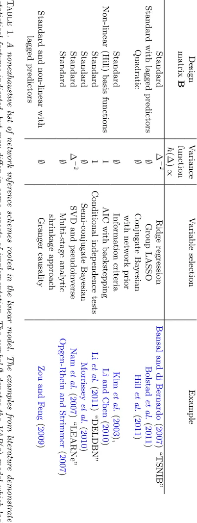
A number of specific network inference schemes can now be recovered by fixing the design matrix and variance function and coupling the resulting model with a variable selection technique. A selection of published network

inference schemes that can viewed in this way is presented in Table1. One

might see these schemes classed as VAR models (Bolstad et al.,2011;

Mor-risseyet al.,2010;Opgen-Rhein and Strimmer,2007;Zou and Feng,2009),

DBNs (Hillet al.,2011;Kimet al.,2003), or ODE-based approaches (Bansal

and di Bernardo, 2007; Li and Chen,2010; Nam et al.,2007), although as we have demonstrated this classification disguises their shared foundation in the linear model.

As shown in Table 1, the variance functions h, and therefore sampling

intervals ∆j, are not treated in a consistent way in the literature. In the

special case of even sampling times ∆j = ∆, a model is characterized only

by its design matrix. If the standard design matrix is used then the entire family of models

Y(tj)−Y(tj−1)

∆ ∼N(AY(tj−1), h(∆)D(σ

2

1, . . . , σP2))

(11)

reduces to a linear VAR(1) model

(13)

[image:13.612.217.418.114.647.2]

(14)

where ¯A= ∆A+Iand ¯σ2

p = ∆2h(∆)σ2p. More generally the VAR(q) model

is prevalent in the literature (see Table 1), yet it does not explicitly

han-dle uneven sampling intervals. This is a potentially important issue since uneven sampling is commonplace in global perturbation experiments, with high frequency sampling used to capture short term cellular response and low frequency sampling to capture the approach to equilibrium. We discuss the importance of modeling using a variance function, and whether a natural

choice for such a function exists in Section4below. In addition we explored

whether inference may be improved through the use of either nonlinear ba-sis functions or lagged predictors to capture respectively nonlinearity and

memory in the underlying drift function is unclear. Section 3 presents an

empirical investigation of these issues.

2.4. Inference. An appealing feature of the discrete time model is that parameters corresponding to different variables are orthogonal in the Fisher sense:

L(θ) =

P

Y

p=1

L(Ap,•, σp)

(13)

As a consequence network inference over G may be factorized intoP

inde-pendent variable selection problems. For definiteness we focus on just two approaches to variable selection, the Bayesian marginal likelihood and AIC, but note that many other approaches are available, including those listed

in Table 1, and can be applied here in analogy to what follows. Below we

assume the response vectordyph−1/2 and the columns of the design matrix

Bh−1/2are standardized to have zero mean and unit variance, but for clarity

subsume this into unaltered notation.

2.4.1. Bayesian variable selection. For simplicity, the variance function

is initially taken to be constant (h= 1). We set up a Bayesian linear model

conditional on a network G using Zellner’s g-prior (Zellner, 1986), that is

with priors Ap,•_|σ2

p ∼ N(0, σp2n(Bp0Bp)−1) and π(σ2p) ∝ 1/σp2 where Bp

is the design matrix B with non-predictors removed according to G. We

note that while the g-prior is a common choice, alternatives may offer some

advantages (Deltell,2011;Friedmanet al.,2000).

Letmp be the number of predictors for variablepin the networkG.

Inte-grating the likelihood (induced by Eqn. 10) against the prior for (Ap,•, σ2

p)

produces the following closed-form marginal likelihood

π(y|G) ∝ Y

p

1

1 +n

mp/2

dy0_pdyp−

n

1 +n

ˆ

dy0_pdˆy_p

−n/2

(15)

where ˆdy_p =Bp(Bp0Bp)−1Bp0dyp. These formulae extend to arbitrary

vari-ance functions h by substituting B _7→ Bh1/2_, _d_y _7→ _d_y_h1/2_{. Network}

in-ference may now be carried out by Bayesian model averaging, using the

posterior probability of a directed edge from variable ito variablej:

P(iregulatesj) =

X

G

π(y_|G)π(G)

P

G0π(y|G0)π(G0)I{

(i, j)_∈E(G)_}.

(15)

In experiments below, we take a network prior which, for each variable p

is uniform over the number of predictors mp up to a maximum permissible

in-degree dmax, that is π(G) ∝ Qp

P mp

−1

I{mp ≤dmax}, but note that

richer subjective network priors are available in the literature (Mukherjee and Speed,2008). Finally, a network estimator ˆGis obtained by thresholding

posterior edge probabilities: (i, j)_∈E( ˆG)_⇔P(iregulatesj)> . For small

maximum in-degreedmax, exact inference by enumeration of variable subsets

may be possible. Otherwise, Markov chain Monte Carlo (MCMC) methods can be used to explore an effectively smaller model space (Ellis and Wong, 2008; Friedman and Koller, 2003). In the experiments below we use exact inference by enumeration.

2.4.2. Variable selection by corrected AIC. Again, consider a constant

variance function (h= 1); rescaling as described above recovers the general

case. The usual maximum likelihood estimates ˆAp,• = (Bp0Bp)−1Bp0dypand

ˆ

σ2 p = n1

P

j(dyp(tj)−dˆyp(tj))2induce closed formsCpσˆp−nfor the maximized

factors of the likelihood function, whereCp is a constant not depending on

the choice of predictors. Corrected AIC scores (Burnham and Anderson, 2002) for each variable pare then

AICc(p, G) =nlog(ˆσ_p2) + 2mp+2mp(mp+ 1)

n−mp−1 . (16)

Again we consider all models with maximum permissible in-degree dmax.

Lowest scoring models are chosen for each variable in turn, inducing a

net-work estimator ˆG.

3. Results. In this Section, we present empirical results investigating the performance of a number of network inference schemes that are special

cases of the general formulation described by Eqn.10. Objective assessment

of network inference is challenging (Prillet al.,2010), since for most

biologi-cal applications the true data-generating network is unknown. We therefore

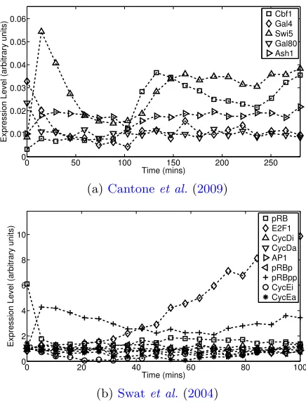
exploit two published dynamical models of biological processes, namely

Can-toneet al. (2009) andSwat et al. (2004), described in detail in

(16)

gene regulatory network built in the yeast Saccharomyces cerevisiae. This five gene network and associated delay differential equations (DDEs) has

received attention in computational biology (Camacho and Collins, 2009;

Minty et al., 2009), and has been shown to agree with gold-standard data

(at least under an E(f(FX)) ≈ f(FE(X)) assumption). Cantone et al.

con-sider two experimental conditions; “switch-on” and “switch-off”. In this pa-per “switch-on” parameter values were used to generate data. The Swat

model is a gene-protein network governing the G1/S transition in

mam-malian cells. The model has a nine dimensional state vector and, unlike Cantone, is Markovian. We note that this model has not been directly ver-ified in the manner of Cantone but is based on a theoretical understanding of cell cycle dynamics. There is undoubtedly bias from this essentially ar-bitrary choice of dynamical systems but a comprehensive sampling of the (vast) space of possible networks and dynamics is beyond the scope of this paper.

3.1. Experimental procedure.

3.1.1. Simulation. We consider global perturbation data by initializing

the dynamical systems from out of equilibrium conditions. This is a common setting for network inference approaches, but the limitations of inference from such data remain incompletely understood. For each dynamical system

f, trajectoriesXk_{of single cell expression levels were obtained as solutions to}

the SDDE Eqn.1 with driftf and uncorrelated diffusion g(X) =σcellD(X)

(representing multiplicative cellular noise). Trajectories were obtained by numerically solving SDDEs with heterogeneous initial conditions using the

Euler-Maruyama discretization scheme (Eqn.4). MATLAB R2010a code for

all simulation experiments is available in the SI. To mimic destructive sam-pling and consequent nonlongitudinality, solutions were regenerated at each time point. We are interested in data that are averages over a large

num-berN of single-cell trajectories. However, the computational cost of solving

N _×n SDDEs to produce each data set is prohibitive. Therefore, only a

smaller number N∗ << N of cells were simulated and a larger sample N

then obtained by bootstrapping, i.e. re-sampling from the N∗ _trajectories

with replacement. In practiceN∗_{should be taken sufficiently large such that}

a negligible change in experimental outcome results from further increase in

N∗. Initial conditions for single cell trajectories varied with standard

de-viation σcell. Finally, uncorrelated Gaussian noise of magnitude σmeas was

added to simulate a measurement process with additive error. In the

exper-iments presented below,N = 10,000, N∗ = 30 and n= 20 time points are

(17)

and 0-100 minutes for Swat). Measurement error and cellular noise are set

to give signal-to-noise ratios_hX_i/σmeas≈10,hXi/σcell ≈10 (herehXi

rep-resents the average expression levels of the variables X over all generated

trajectories). Fig.1 shows typical datasets for the two dynamical systems.

3.1.2. Inference schemes. The following inference schemes were assessed

Variable Selection _{ Bayesian, AICc }

Design matrix _{ Standard, Quadratic _}

Lagged predictors { No, Yes }

Variance functionh(∆)_∝∆−α α=_{ 0, 1, 2 ,_{∅ }}

For the design matrix “quadratic” refers to the augmentation of the pre-dictor set by the pairwise products of prepre-dictors, the simplest nonlinear

basis functions. For the variance function the symbol∅is used to denote the

VAR(q) model, which formally lacks a variance function. “Lagged predictors

= Yes” indicates augmentation of the predictor set with lagged observations

(a lag of ≈ 28 mins is used for Cantone and ≈ 10 mins for Swat). There

are heuristic justifications for each of the candidate variance functions. For

example the function withα= 2 appears for small ∆j when an exact Euler

approximation and additive measurement error are assumed (Bansal and di Bernardo, 2007), whereas α = 1 is reminiscent of the Euler-Maruyama

discretization Eqn. 4.

3.1.3. Empirical assessment. The performance of each inference scheme

is quantified by the area under the receiver operating characteristic (ROC)

curve (AUR), averaged over 20 datasets (Fawcett,2005). This metric,

equiv-alent to the probability that a randomly chosen true edge is preferred by the inference scheme to a randomly chosen false edge, summarizes, across a range of thresholds, the ability to select edges in the true data-generating graph. Results presented below use a computationally favorable in-degree

re-strictiondmax= 2. In order to check robustness todmaxall experiments were

repeated usingdmax= 3, with no substantial changes in observed outcome

(SFig. 6).

3.2. Empirical results.

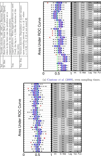
3.2.1. Even sampling interval. Fig. 2(a) displays box-plots over AUR

(18)

0 50 100 150 200 250 0

0.01 0.02 0.03 0.04 0.05 0.06

Time (mins)

Expression Level (arbitrary units)

Cbf1 Gal4 Swi5 Gal80 Ash1

(a)Cantoneet al.(2009)

0 20 40 60 80 100

0 2 4 6 8 10

Time (mins)

Expression Level (arbitrary units)

pRB E2F1 CycDi CycDa AP1 pRBp pRBpp CycEi CycEa

(b)Swatet al.(2004)

Fig 1. Two published dynamical systems models of cellular processes were used to generate datasets. Single cell trajectories were generated from an SDDE model (Eqn.1) and averaged under measurement noise and nonlongitudinality due to destructive sampling. (a) Data generated from (a model due to)Cantone et al. (2009), describing a synthetic network built in yeast. (b) Data generated from Swat et al. (2004), a theory-driven model of the G1/S transition in mammalian cells.

the VAR model, since the parameters A carry a subtly different meaning,

which under a Bayesian formulation leads to a translation of the prior dis-tribution and in the information criteria case changes the definition of the predictor set.)

Despite the presence of nonlinearities and memory in the cellular driftf,

[image:18.612.193.411.119.405.2]

(19)

Inf. V ariable sele ction. AIC [AIC] or Ba y esian [Ba yes]. D. Mat. Basis functions. Linear [Std] or quadratic [Quad], where in the latter case the predictor set is augmen ted b y the pairwise pro ducts. Lag L agge d pr edictors. When lagged predictors are used [Used], the lag is ≈ 1 / 10th the dur ation of the time series. V ar. F un. V arianc e function. Dep endence of m o del variance up on sampling in terv al, h (∆) ∝ ∆ − α where α = 0 [0], 1 [1], 2 [2] or not stated [ ∅ ]. 1

0

0.5

1 Area Under ROC Curve

AIC Quad None x AIC Quad None 2 AIC Quad None 1 AIC Quad None 0 AIC Quad Used x AIC Quad Used 2 AIC Quad Used 1 AIC Quad Used 0 AIC Std None x AIC Std None 2 AIC Std None 1 AIC Std None 0 AIC Std Used x AIC Std Used 2 AIC Std Used 1 AIC Std Used 0 Bayes Quad None x Bayes Quad None 2 Bayes Quad None 1 Bayes Quad None 0 Bayes Quad Used x Bayes Quad Used 2 Bayes Quad Used 1 Bayes Quad Used 0 Bayes Std None x Bayes Std None 2 Bayes Std None 1 Bayes Std None 0 Bayes Std Used x Bayes Std Used 2 Bayes Std Used 1 Bayes Std Used 0

Inf. D. Mat Lag Var. Fun.

(a)Cantoneet al.(2009), even sampling times.

0

0.5

1 Area Under ROC Curve

(b)Cantoneet al.(2009), uneven sampling times.

[image:19.612.143.476.114.627.2]

(20)

0

0.5

1 Area Under ROC Curve

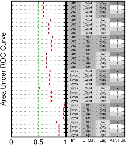
Fig 3. Investigation of empirical consistency of network estimators, using theCantone et

al.(2009) model with even sampling intervals. Area under ROC curves are shown in the large dataset, zero cellular heterogeneity and zero measurement noise limits.

Corresponding results for the Swat model are shown in SFig. 2. Here we find that none of the methods performs well.

We also performed inference using biochemical data from the

experimen-tal system reported in Cantone et al. (2009) (specifically the “switch-on”

dataset therein). AUR scores obtained using this data (SFig. 5) were in close

agreement with those obtained using synthetic data (Fig.2(a)), suggesting

that the results of the simulations are relevant to real world studies.

3.2.2. Uneven sampling intervals. Many biological time-course

experi-ments are carried out with uneven sampling intervals. We therefore repeated the analysis above with sampling times of 0, 1, 5, 10, 15, 20, 30, 40, 50, 60,

75, 90, 105, 120, 140, 160, 180, 210, 240 and 280 minutes. Fig.2(b) displays

[image:20.612.194.405.117.363.2]

(21)

3.2.3. Consistency. Fig. 3 displays AUR scores for Cantone for a large

number of evenly sampled time points (n= 100), and the limiting case of

zero measurement noise and zero cellular heterogeneity (σmeas= 0,σcell = 0,

even sampling intervals). Consistency (in the sense of asymptotic conver-gence of the network estimate to the data-generating network) may be unattainable due to the nonidentifiability resulting from limited exploration of the dynamical phase space. This lack of surjectivity means that in many cases inference cannot possibly reveal the full data-generating graph, al-though as we have seen network inference can nonetheless be informative.

From Fig. 3 we see that the Bayesian schemes using linear predictors

ap-proach AUR equal to unity, and in this sense show empirical consistency with respect to network inference. However, some of the other methods do not converge to the correct graph even in this limit.

4. Discussion. The analyses presented here were aimed at better un-derstanding statistical network inference for biological applications. We showed how a broad class of approaches, including VAR models, linear DBNs and certain ODE-based approaches, are related to stochastic dynamics at the cellular level. We discuss a number of these aspects below and close with some views on future perspectives for network inference, including recom-mendations for practitioners.

4.1. Time intervals. We found that uneven sampling intervals posed problems, even for methods that explicitly accounted for the sampling in-terval. Further insight may be gained from a “propagation of uncertainty”

analysis of the approximations indicated in Section2.2. Assuming the true

large sample process obeys dX∞/dt=F(X∞), we have that under an

ob-servation process with independent additive Gaussian measurement error

Y(t)_∼ N(X∞(t),M) an expansion for the variance V(dY−F(Y)) over a

time interval ∆ is given by

M∆−2+ (I∆−1+DF)M(I∆−1+DF)0+. . .

(17)

(see SI for details). Recall that the model family in Eqn.10approximates this

variance by h(∆)_D(σ2

1, . . . , σP2) where h(∆) = ∆−α. From this perspective

it is clear that each variance function we considered captures only partial variation due to ∆. It is therefore not surprising that performance suffers in the uneven sampling regime, which requires the variance function to apply equally to large ∆ as to small ∆. Moreover, a natural choice of variance

function driven by Eqn.17is not possible, since this would require knowledge

(22)

absent specific reasons for uneven sampling, it may be preferable to collect data at regular intervals.

0 5 10 15

10−1

100

101

102

Time Step ∆ (mins)

Variance Function h(

∆

)

(arbitrary units)

h

true h ∝ 1 h ∝∆−1 h ∝∆−2

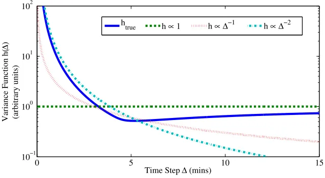
Fig 4. Variance functions used in literature provide partial approximation to the “true”

functional form forCantone et al.(2009). For small time steps a power law∆−α provides a good approximation, but for larger time steps a constant variance function may be more appropriate. In practice the precise form ofhtruewill be unknown.

Fig. 4 displays an approximation to the true variance function for the

Cantone model (see SI). Observe that for small sampling intervals ∆ the true curvature is best captured by a functional approximation of the form

h(∆)_∝∆−α _with_α_{= 1}_,_{2, whereas for intervals larger than 10 mins (which}

are more common in practice) the flat approximation h(∆) ∝ 1 correctly

captures the asymptotic behavior. In applications where high frequency sam-pling is infeasible the flat variance function might be a sensible choice. To understand whether difficulties related to sampling intervals disappear in the large sample limit, we repeated the empirical consistency analysis under uneven sampling (SFigs. 11,12). Interestingly, we found that none of the methods appeared to be empirically consistent, and that the choice of vari-ance function is influential. However, unevenly sampled data are common in biology and it may be the case that in some settings, the existence of multiple time scales (e.g. signaling, transcription, accumulating epigenetic alterations) mean that unevenly sampled data are nonetheless useful. Our findings suggest that care should be taken in the uneven sampling regime.

[image:22.612.136.456.159.334.2]

(23)

per-turbation, exploring a large proportion of the dynamical phase space. How-ever such behavior is dependent on the specific dynamical system and is not displayed by the Swat model, which has a much larger phase space, being a nine-dimensional dynamical system. This may help explain the poor per-formance of all the methods on this latter model using global perturbation data and perhaps reinforces the intuitive notion that dynamics that are fa-vorable (in this informal sense) facilitate network inference. In some cases, perturbation data are available in which individual variables are inhibited (e.g. by RNA interference, gene knockouts or inhibitor treatments). Such data have the potential to explore much more of the dynamical phase space, including regions which cannot be accessed without direct inhibition of spe-cific molecular components. This is an important consideration because the

statistical estimators described in Section 2.4take the form

ˆ

A=hDf(FX)iX∈R

(18)

where the average is over the region _{R ⊆ X} in state space visited during

the experiments. Clearly if the region (f(FR),R) is only a small subspace of

phase space then the estimate Eqn.18 will be poor compared to one based

on the entire phase space ˆA∗ =_hDf(_FX)iX∈X.

To investigate the added value of interventional treatments for network inference, we repeated both the Cantone and Swat analyses with an ensem-ble of datasets obtained by inhibiting each variaensem-ble in turn; this gave 5 and 9 datasets for Cantone and Swat respectively. Whilst no improvement to the Cantone AUR scores was observed (SFig. 15), there was improved per-formance for Swat (SFig. 16). This suggests that global perturbations are insufficient to explore the Swat dynamical phase space, and supports the intuitive notion that intervention experiments may be essential for infer-ence regarding larger dynamical systems. Nevertheless AUR scores remain far from unity. This may be because the Swat drift function contains com-plex interaction terms which single interventions alone fail to elucidate. An important problem in experimental design will be to estimate how much (possibly combinatorial) intervention is required to achieve a certain level of network inference performance.

We considered precise artificial intervention of single componentsin silico.

(24)

There remains a need for novel statistical methodology capable of analyzing time-course data under biological interventions. Existing literature in causal

inference (Pearl, 2009) and related work in graphical models (Eaton and

Murphy, 2007) are relevant, but in biological applications it may also be important to consider the mechanism of action of specific interventions.

4.3. Non-linear models. We focused on linear statistical models. Clearly,

linear models are inadequate in many cases. For exampleRogerset al.(2007)

demonstrate the benefit of a nonlinear model based on Michaelis-Menten chemical kinetics for inference of transcription factor activity. However,

net-work inference based on nonlinear ODEs remains challenging (Xu et al.,

2010). AlternativelyAij¨¨ o and L¨ahdesm¨aki(2009) consider the use of a non-parametric Gaussian process (GP) interaction term in the regression, which is naturally more flexible than linear regression using finitely many basis functions. This may help to overcome the linearity restriction, but intro-duces additional degrees of freedom, including the GP covariance function and associated hyperparameters. Whilst a thorough comparison of such ap-proaches was beyond the scope of this article, the potential utility of non-parametric interaction terms is worthy of investigation. In this study we observed that neither the use of predictor products nor lagged predictors led to improved performance; this may reflect nontrivial coupling between cellular dynamics and the observed data.

4.4. Single-cell data. In the future it may become possible to measure

single cell expression levels Xk non-destructively (e.g. by live cell

imag-ing), producing truly longitudinal datasets. It is interesting to consider how such data may impact upon the performance of regression-based net-work inference. Under independent additive Gaussian measurement error

Y(t) _∼ N(Xk(t),M) an expansion for the single cell variance V(dY−f)

over a time interval ∆, in analogy with Eqn.17, is given by

M∆−2+ (I∆−1+DF)M(I∆−1+DF)0+ ∆−1gg0+. . .

(19)

(see SI). Thus a (single) longitudinal single cell dataset contains less

in-formation about the drift f than aggregate data (Eqn. 17) due to cellular

stochasticityg. However, multiple longitudinal datasets may jointly contain

(25)

scores, but reduction by a factor of about two in the variance of these scores (compared with the corresponding non-longitudinal data), implying that the network estimators may be converging to an incorrect network. Bias may

occur when the cellular driftf is not well approximated by a linear function,

as is the case for the Swat model. Consider the idealized scenario where

f _≡f(X) is Markovian and it is possible to observe longitudinal, single cell

expression levels. Under these apparently favorable circumstances even es-timators obtained after a thorough exploration of state space may not offer

good approximations, i.e. ˆA∗ _6≈ Df_|_x₌₀. As a toy example consider the

cellular drift

f : [0,1]2_→R, f(X) =

(2π)−1sin(2πX2)

(2π)−1_sin(2_πX

1)

(20)

which is not well approximated by a linear function over the state space

X = [0,1]2_{. In this case averaging leads to cancellation}

ˆ

A∗ =_hDf(X)_iX∈X =

0 cos(2πX2)

cos(2πX1) 0

X∈[0,1]2 (21)

= 06=

0 1 1 0

= Df|x=0

so that no interactions are inferred. Under such circumstances network in-ference is no longer possible using the na¨ıve linear regression approach. This suggests that network inference rooted in non-linear models may be needed to fully exploit longitudinal single-cell data in the future. A related line of work addresses heterogeneity of the drift function in time by coupling DBNs

with change point processes (Grzegorczyk and Husmeier,2010;Kolaret al.,

2009; L`ebreet al.,,2010). A promising direction would be piecewise linear regression modeling for network inference applications, where the hetero-geneity appears in the spatial domain.

4.5. High-dimensions and missing variables. We focused on the simplest possible case of fully observed, low-dimensional systems. There is a rich lit-erature in high-dimensional variable selection and related graphical

mod-els (Meinshausen and B¨uhlmann, 2006; Hans et al., 2007;Friedman et al.,

(26)

This may be acceptable for the purpose of predicting the outcome of bio-chemical interventions (e.g. inhibiting gene or protein nodes), but limits stronger causal or mechanistic interpretations. Latent variable approaches

are available (Bealet al.,2005), but model selection can be challenging and

remains an open area of research (Knowles and Ghahramani,2011). We note

also that the missing variable issue for biological networks is arguably more severe than in, say, economics or epidemiology, insofar as measured variables may represent only a small fraction of the true state vector, often with little specific insight available into the nature of the missing variables or their relationship to observations. Further work is required to better understand these issues in the context of inference for biological networks.

4.6. Future perspectives. We found that a simple linear model could suc-cessfully infer network structure using globally perturbed time-course data from the Cantone system. It is encouraging that inference based only on as-sociations between variables, none of which were explicitly intervened upon, can in some cases be effective. Interventional designs should further enhance prospects for network inference. On the other hand, theoretical arguments, and the results we showed from the Swat system, emphasize that in some cases network structure may not be identifiable, even at the coarse level re-quired for qualitative biological prediction. On balance, we believe that net-work inference can be useful in generating biological hypotheses and guiding further experiment. However, the concerns we raise motivate a need for cau-tion in statistical analysis and interpretacau-tion of results. At the present time, we do not believe network inference should be treated as a routine analysis in bioinformatics applications, but rather as an open research area that may, in future, yield standard experimental and statistical protocols.

Some specific recommendations that arise from the results presented here are:

• A default model. Our results suggest that a reasonable default choice of model for typical applications uses the standard design matrix with no lagged predictors and a flat variance function, corresponding to the linear model

dY(tj)∼N(AY(tj−1),D(σ2₁, . . . , σ_P2)).

(22)

Coupled with the Bayesian variable selection scheme outlined in Sec-tion2.4.1, this simple model produced empirically consistent network estimators for Cantone using evenly sampled global perturbation data

(27)

• Diagnostics and validation. It is clear that network inference does not enjoy general theoretical guarantees and that the ability to successfully elucidate network structure depends on details of the specific system under study. Therefore careful empirical validation on a case-by-case basis is essential. This should include statistical assessment of model fit, robustness and predictive ability and where possible systematic validation using independent interventional data.

• Experimental design. We suggest sampling evenly in time as a de-fault choice. Interventional designs may be helpful to effectively ex-plore larger dynamical phase spaces. However, to control the burden of experimentally exploring multiple time points, molecular species, interventions, culture conditions and biological samples, adaptive de-signs that prune experiments based on informativeness for the specific

biological setting may be helpful (Xu et al.,2010).

In conclusion, linear statistical models for networks are closely related to models of cellular dynamics and can shed light on patterns of biochem-ical regulation. However, biologbiochem-ical network inference remains profoundly challenging, and in some cases may not be possible even in principle. Nev-ertheless, studies aimed at elucidating networks from high-throughput data are now commonplace and play a prominent role in biology. For this reason there remains an urgent need for both new methodology and theoretical and empirical investigation of existing approaches. Furthermore, there re-main many open questions in experimental design and analysis of designed experiments in this setting.

Acknowledgements. We would like to thank Prof K. Kafadar and the anonymous referees for constructive suggestions that helped to improve the content and presentation of this article, and G. O. Roberts, S. Spencer and S. M. Hill for discussion and comments. We wish to acknowledge the support of EPSRC EP/E501311/1 (CJO & SM) and NCI U54 CA 112970 (SM).

SUPPLEMENTARY MATERIAL

Supplement: Additional Materials

(INSERT WEB ADDRESS HERE). This supplement provides the dynami-cal systems used in this paper and accompanying MATLAB R2010a scripts, derivations and additional figures SFig. 1-16.

References.

¨

(28)

Altay, G., Emmert- Streib, F. (2010) Revealing differences in gene network inference algo-rithms on the network level by ensemble methods,Bioinformatics,26(14), 1738-1744. Babu, M.M., Luscombe, N.M., Aravind, L.,et al.(2004) Structure and evolution of

tran-scriptional regulatory networks,Current Opinion in Structural Biology,14(3), 283-91. Bansal, M., di Bernardo, D. (2007) Inference of gene networks from temporal gene

expres-sion profiles,IET Systems Biology,5, 306-12.

Bansal, M., Belcastro, V., Ambesi-Impiombato, A.et al.(2007) How to infer gene networks from expression profiles,Mol. Sys. Bio.,3(78).

Beal, M.J., Falciani, F. Ghahramani, Z.,et al.(2005) A Bayesian approach to reconstruct-ing genetic regulatory networks with hidden factors,Bioinformatics,21(3), 349. Bolstad, A., Van Veen, B., Nowak, R. (2011) Causal Network Inference via Group Sparse

Regularization,IEEE Trans. Signal Processing,99.

Bonneau, R. (2008) Learning biological networks: from modules to dynamics,Nat. Chem. Bio.,4, 658-64.

Burnham, K.P., Anderson, D.R. (2002) Model Selection and Multimodal Inference: A Practical Information-Theoretic Approach, Springer, New York.

Camacho, D.M., Collins, J.J. (2009) Systems biology strikes gold,Cell,137(1), 24- 6. Cantone, I., Marucci, L., Iorio, F., et al. (2009) A yeast synthetic network for in vivo

assessment of reverse-engineering and modeling approaches,Cell,137(1), 172-81. Craciun, G., Pantea, C. (2008) Identifiability of chemical reaction networks, J. Math.

Chem.,44, 244-59.

Dargatz, C. (2010) Bayesian Inference for Diffusion Processes with Applications in Life Sciences, PhD Thesis, M¨unchen.

Davidson, E.H. (2001) Gene Regulatory Systems. Development And Evolution, Academic Press, San Diego, 2001.

Deltell, A. (2011) Objective Bayes Criteria for Variable Selection,PhD thesis, Universitat de Valencia.

Eaton, D., Murphy, K. (2007) Exact Bayesian structure learning from uncertain in-terventions, Proceedings of 11th Conference on Artificial Intelligence and Statistics (AISTATS- 07).

Ellis, B, Wong, W.H. (2008) Learning causal Bayesian network structures from experi-mental data,JASA,103(482), 778-89.

Elowitz, M.B., Levine, A.J., Siggia, E.D., et al.(2002) Stochastic gene expression in a single cell,Science,297(5584), 1129-31.

Fawcett, T. (2005) An introduction to ROC analysis, Pattern Recognition Letters, 27, 861-874.

Friedman, N., Linial, M., Nachman, I.,et al.(2000) Using Bayesian networks to analyze expression data,J. Comp. Bio.,7, 601-620.

Friedman, J., Hastie, T., Tibshirani, R. (2008) Sparse inverse covariance estimation with the graphical lasso,Biostatistics,9(3), 432.

Friedman, J, Koller, D. (2003) Being Bayesian about network structure. A Bayesian ap-proach to structure discovery in Bayesian networks,Machine Learning,50(1), 95-125. Hache, H., Lehrach, H., Herwig, R. (2009) Reverse Engineering of Gene Regulatory

Net-works: A Comparative Study,EURASIP Journal on Bioinformatics and Systems Biol-ogy, 617281.

Hans, C. and Dobra, A. and West, M. (2007) Shotgun stochastic search for “large p” regression,Journal of the American Statistical Association,102(478), 507-516. Hecker, M., Lambeck, S., Toepfer, S., et al. (2009) Gene regulatory network inference:

Data integration in dynamic models - A review,Biosystems,96(1), 86-103.

(29)

in a Single Cancer, In preparation.

Hurn, A., Jeisman, J., Lindsay, K. (2007) Seeing the wood for the trees: A critical evalua-tion of methods to estimate the parameters of stochastic differential equaevalua-tions,Journal of Financial Econometrics,5(3), 390.

Grzegorczyk, M., Husmeier, D. (2010) Improvements in the reconstruction of time-varying gene regulatory networks: dynamic programming and regularization by information sharing among genes,Bioinformatics,27(5), 693-9.

Ideker, T., Lauffenburger, D. (2003) Building with a scaffold: emerging strategies for high to low level cellular modelling,Trends in Biotechnology,21(6), 255-62.

Kim, S.Y., Imoto, S., Miyano, S. (2003) Inferring gene networks from time series microar-ray data using dynamic Bayesian networks,Briefings in Bioinformatics,4(3), 228- 35. Knowles, D.A., Ghahramani, Z. (2011) Nonparametric Bayesian Sparse Factor Models

with Application to Gene Expression Modelling,AOAS,5(2B), 1534-52.

Kolar, M., Song, L., Xing, E.P. (2009) Sparsistent learning of varying-coefficient models with structural changes,NIPS,22, 100614.

Kou, S., Sunney, X., Jun, L. (2005) Bayesian analysis of single-molecule experimental data (with discussion),J. Roy. Statist. Soc., C,54, 469-506.

L`ebre, S., Becq, J., Devaux, F.et al.(2010) Statistical inference of the time-varying struc-ture of gene- regulation networks,BMC Systems Biology,4, 130.

Lee, W.P., Tzou, W.S. (2009) Computational methods for discovering gene networks from expression data,Brief. Bioinform.,10(4), 408-423.

Li, C-W., Chen, B-S. (2010) Identifying Functional Mechanisms of Gene and Protein Regulatory Networks in Response to a Broader Range of Environmental Stresses,Comp. and Func. Genomics, 408705.

Li, Z., Li, P., Krishnan, A. (2011) Large-scale dynamic gene regulatory network inference combining differential equation models with local dynamic Bayesian network analysis,

Bioinformatics,27(19), 2686-91.

Marbach, D., Schaffter, T., Mattiussi, C.,et al.(2009) Generating realistic in silico gene networks for performance assessment of reverse engineering methods,Journal of com-putational biology,16(2), 229-39.

Markowetz, F., Spang, R. (2007) Inferring cellular networks - A review,BMC Bioinfor-matics,8(Suppl. 6), S5.

McAdams, H.H., Arkin, A. (1997) Stochastic mechanisms in gene expression,PNAS,94, 814-9.

Meinshausen, N., B¨uhlmann, P. (2006) High-dimensional graphs and variable selection with the lasso,The Annals of Statistics,34(3), 1436-62.

Minty, J.J., Varedi, K.S.M., Nina, L.X. (2009) Network benchmarking: a happy marriage between systems and synthetic biology,Chemistry and Biology,16(3), 239-41. Morrissey, E.R., Ju´arez, M.A., Denby, K.J.,et al.(2010) On reverse engineering of gene

in-teraction networks using time course data with repeated measurements,Bioinformatics,

26(18), 2305-2312.

Mukherjee, S., Speed, T.P. (2008) Network inference using informative priors, PNAS,

105(38), 14313-8.

Nam, D., Yoon, S.H., Kim, J.F. (2007) Ensemble learning of genetic networks from time-series expression data,Bioinformatics,23(23), 3225-3231.

Oates, C.J. and Mukherjee, S. (2011) Supplement to “Biological Dynamics and Network Inference”.

Øksendal, B. (1998) Stochastic Differential Equations, An Introduction with Applications, 5th ed., Springer.

(30)

time course data: an effective model selection procedure for the vector autoregressive process,BMC Bioinformatics,8, (Suppl. 2), S3.

Pearl, J. (2009) Causal inference in statistics: An overview,Statistical Surveys,3, 96-146. Prill, R.J., Marbach, D., Saez- Rodriguez,et al.(2010) Towards a rigorous assessment of

systems biology models: the DREAM3 challenges,PloS one,5, e9202.

Paulsson, J. (2005) Models of stochastic gene expression,Physics of Life Reviews,2(2), 157-75.

Rogers, S., Khanin, R., Girolami, M. (2007) Bayesian model-based inference of transcrip-tion factor activity,BMC Bioinformatics,8(S2).

Schoeberl, B., Eichler-Jonsson, C., Gilles, E.D.,et al.(2002) Computational modeling of the dynamics of the MAP kinase cascade activated by surface and internalized EGF receptors,Nature Biotechnology,20(4), 370-5.

Smith, V.A., Jarvis, E.D., Hartemink, A.J. (2002) Evaluating functional network inference using simulations of complex biological systems,Bioinformatics,18(S1), S216-S224. Swain, P.S., Elowitz, M.B., Siggia, E.D. (2002) Intrinsic and extrinsic contributions to

stochasticity in gene expression,PNAS,99, 12795-800.

Swat, M., Kel, A., Herzel, H. (2004) Bifurcation analysis of the regulatory modules of the mammalian G1/S transition,Bioinformatics,20(10), 1506-11.

Van den Bulcke, T., Van Leemput, K., Naudts, B.,et al.(2006) SynTReN: a generator of synthetic gene expression data for design and analysis of structure learning algorithms,

BMC Bioinformatics,7(43).

Van Kampen, N.G. (2007) Stochastic Processes in Physics and Chemistry, North Holland, Third Edition.

Werhli, A.V., Grzegorczyk, M., Husmeier, D. (2006) Comparative evaluation of reverse en-gineering gene regulatory networks with relevance networks, graphical gaussian models and bayesian networks,Bioinformatics,22(20), 2523-31.

Wilkinson, D.J. (2006) Stochastic Modelling for Systems Biology,Mathematical and Com-putational Biology, Chapman and Hall/CRC, ISBN: 1-58488-540-8.

Wilkinson, D.J. (2009) Stochastic modelling for quantitative description of heterogeneous biological systems,Nature Reviews Genetics,10(2), 122- 33.

Xu, T.R., Vyshemirsky V., Gormand A.,et al.(2010) Inferring signaling pathway topolo-gies from multiple perturbation measurements of specific biochemical species,Science Signaling,3(113), ra20.

Yarden, Y., Sliwkowski, M.X. (2001) Untangling the ErbB signalling network, Nature Reviews Molecular Cell Biology,2, 127-37.

Zellner, A. (1986) On Assessing Prior Distributions and Bayesian Regression Analysis With g-Prior Distributions, Bayesian Inference and Decision Techniques - Essays in Honor of Bruno de Finetti, eds. P. K. Goel and A. Zellner, 233-24.

Zou, C., Feng, J. (2009) Granger causality vs. dynamic Bayesian network inference: a comparative study,BMC Bioinformatics,10(12).

Centre for Complexity Science University of Warwick

Coventry, CV4 7AL, UK E-mail:[email protected]

Department of Statistics University of Warwick Coventry, CV4 7AL, UK

E-mail:[email protected]

Department of Biochemistry Netherlands Cancer Institute 1066CX Amsterdam, Netherlands E-mail:[email protected]