An effective genetic algorithm for network coding

University of Warwick institutional repository: http://go.warwick.ac.uk/wrap

This paper is made available online in accordance with publisher policies. Please scroll down to view the document itself. Please refer to the repository record for this item and our policy information available from the repository home page for further information.

To see the final version of this paper please visit the publisher’s website. Access to the published version may require a subscription.

Author(s): Xiao-Bing Hu, Mark S. Leeson, and Evor L. Hines, Article Title: An effective genetic algorithm for network coding Year of publication: 2011

Link to published article: http;//dx.doi.org/10.1016/j.cor.2011.07.014 Publisher statement: NOTICE: this is the author’s version of a work that was accepted for publication in Computers & Operations

Research. Changes resulting from the publishing process, such as peer review, editing, corrections, structural formatting, and other quality control mechanisms may not be reflected in this document. Changes may have been made to this work since it was submitted for

publication. A definitive version was subsequently published in Computers & Operations Research, VOL39, ISSUE5,

An Effective Genetic Algorithm for

Network Coding

Xiao-Bing Hu, Mark S. Leeson and Evor L. Hines

d

A previous version on the preliminary results of this study was presented at CEC2009, Trondheim, Norway, 18th-21st May 2009.

Abstract— The network coding problem (NCP), which aims to minimize network coding

resources such as nodes and links, is a relatively new application of genetic algorithms (GAs) and

hence little work has so far been reported in this area. Most of the existing literature on NCP has

concentrated primarily on the static network coding problem (SNCP). There is a common

assumption in work to date that a target rate is always achievable at every sink as long as coding is

allowed at all nodes. In most real-world networks, such as wireless networks, any link could be

disconnected at any time. This implies that every time a change occurs in the network topology, a

new target rate must be determined. The SNCP software implementation then has to be re-run to

try to optimize the coding based on the new target rate. In contrast, the GA proposed in this paper

is designed with the dynamic network coding problem (DNCP) as the major concern. To this end, a

more general formulation of the NCP is described. The new NCP model considers not only the

minimization of network coding resources but also the maximization of the rate actually achieved

at sinks. This is particularly important to the DNCP, where the target rate may become

unachievable due to network topology changes. Based on the new NCP model, an effective GA is

designed by integrating selected new problem-specific heuristic rules into the evolutionary process

in order to better diversify chromosomes. In dynamic environments, the new GA does not need to

recalculate target rate and also exhibits some degree of robustness against network topology

changes. Comparative experiments on both SNCP and DNCP illustrate the effectiveness of our new

model and algorithm.

Keywords—Network Coding, Genetic Algorithm, Resource Minimization, Heuristic Rule.

I. INTRODUCTION

The notion of coding at the packet level –commonly called network coding –has attracted significant

now established that network coding may significantly improve network performance in terms of network

throughput. It should be noted that conventional network optimization aims to maximize information flow

by utilizing as much link capacity as possible, whilst network coding begins with the assumption that full

link capacity utilization has already been achieved wherever possible and then attempts to further increase

the network throughput at sinks by performing coding at nodes. This advantage of network coding can be

understood in the context of the example shown in Fig.1.(a) and Fig.1.(b). It is assumed in Fig.1 that two

different pieces of one-unit-sized data/packets, α and β, are to be sent from the source node 1 to the sink node 6 and 7, and the capacity of every link is just 1 (in this paper, the link capacity is defined as the same

as the one in conventional network optimization [1], all data are one-unit-sized, and all links are of

unit-capacity). The aim is to maximize the rate achieved at each sink, i.e., the amount of different data

received by a sink at one time. The rate is also measured in data units. Since all links are of unit-capacity,

the potential maximal achievable rate at a sink is equivalent to the number of its incoming links. However,

different links may carry the same data, such as the two incoming links of node 7 in Fig.1.(a) and so the

actually achieved rate at a sink may be less than the potential rate. This is likely to be the case if the nodes

in the network only forward and replicate the data they receive. For example, as illustrated in Fig.1(a), the

sink node 7 can only receive 1 unit of data β at one time, although the other sink node 6 achieves a rate of 2 by receiving both α and β. The information flow in Fig.1(a) is optimal from the conventional point of view because every link carries one unit of data, which gives a full utilization of the link capacity.

However, if node 4 can combine data from its two incoming links through the ―+‖ operation, then by using

the ―-‖ operation to decode data, a rate of 2 can be achieved at both sinks, as shown in Fig.1.(b). It should

be noted that the result of operation ―+‖, e.g., α+β in Fig.1.(b), is still a one-unit-sized data element. Therefore, without exceeding the link capacity, network coding increases the total rate of information

Although network coding may be allowed at all nodes in some of the relevant literature, an interesting

observation is that a given target rate can often be achieved by conducting network coding at only a

relatively small proportion of the nodes [2]. For instance, in the network given by Fig.1(c), network

coding at both nodes 4 and 5 will make no difference in terms of the rate achieved at the sinks or in other

word, network coding is not necessary in that network. Therefore, a question is raised: at which nodes

does network coding need to be conducted, or how does one make most of network capacity at a minimal

cost in terms of network coding resources? To answer this question, a minimal set of nodes needs to be

found for coding, and this has been proved to be an NP-hard problem [3]. In this paper, the above problem

of minimizing network coding resources is referred to as the Network Coding Problem (NCP). Some

attempts have already been made using different methods to address this problem. For instance, two

minimal approaches were reported in [4] and [5] which ascertain the minimal set of nodes for network

coding in order to achieve a given target rate. It was determined in [4] that coding is required at no more

than d-1 nodes in acyclic networks with 2 unit-rate sources and d sinks. An upper bound on the number of nodes required for both acyclic and cyclic networks was derived in [5]. However, the approaches in both

[4] and [5] determine the minimal set of nodes for coding by removing links in a greedy fashion. A linear

programming method was reported in [6] to optimize the various resources used for network coding, and

α β

α

α

β

β α+β

α+β α+β

(b)

α β

α

α

β

β α

β α

(c) β α β

α

α

β

β β

β β

(a) 1

2 3

4

5

6 7

1

2 3

4

5

6 7

1

2 3

4

5

6 7

its optimal formulations involved a number of variables and constraints that grow exponentially with the

number of sinks.

As large-scale parallel stochastic search and optimization algorithms, genetic algorithms (GAs) have a

good provenance in the resolution of diverse NP-hard problems [7], [8], including network optimization

and resource assignment [9], [10]. However, the optimization of network coding is a relatively new area

for GAs, and very few results have been reported [2], [11], [12], [13] to date. The first attempt to apply

GAs to network coding was made by Kim et al. [2]. This was then extended from acyclic networks to cyclic networks and from centralized cases to decentralized cases [11]. The genetic representation was the

particular focus in later work [12], followed by the proposal of a distributed algorithm to improve GA

computational efficiency [13].

There is a common assumption in the network coding optimization work to date that the target rate is

always achievable if coding is allowed at all nodes, permitting attention to be focused on the minimization

of the number of coding links/nodes. However, in dynamic environments, such as wireless networks, it is

quite possible that the target rate may become unachievable due to uncertainty in the connections between

the nodes [14]. If this is the case, it is the rate that is actually achieved rather than the target rate that plays

a more important role in network coding. The previous studies using the assumption that the target rate

was achievable, such as [2], [4]-[13], did not consider the rate actually achieved when minimizing

resources, and were therefore largely limited to the static NCP (SNCP). They may only be applied to the

dynamic NCP (DNCP) by recalculating the target rate and then re-optimizing resources every time a

change occurs in the network topology.

Network coding in dynamic environments is a challenging research topic. Random network coding has

proved to be very promising in coping with network topology changes, as it does not require the

knowledge of the entire network topology [15]-[19]. However, in these random network coding studies

the minimization of coding resources is not a concern and each node has to communicate its coding

transmit the signals sent by the source. Therefore, whilst the advantages of random network coding should

be acknowledged, it is still necessary to investigate how to improve network coding based on the entire

network topology. Robustness against changes in network topology will be a particular concern. As will

be explained in Section III, the DNCP model proposed in this paper exhibits such robustness to some

extent when compared with previous work [2], [11].

In our previous study [20], preliminary results relating to the design of effective GAs for the

minimization of coding resources in the NCP, particularly in the DNCP, were reported but the work was

restricted to the NCP utilizing only the simplest addition coding (i.e., the field size is 2) between two

incoming signals. The work presented in this paper is concerned with further developments of our

previous results by extending our work to NCP where coding with any finite field size is adopted to

combine any finite number of incoming signals.

II. PROBLEM FORMULATION

For the sake of simplicity but without losing generality, this paper considers only the

one-source-multi-sink NCP, and it is assumed that the source is always node 1 in the network. Let

G(V(t),E(t),t) denote the network at time instant t, where V(t) and E(t) are sets of vertices and edges. Suppose G has nn nodes, nl links, and ns sinks, and RTarget is the target rate which is expected to be achieved

at every sink.

Before presenting our new NCP model, we would like to give a brief discussion of previous SNCP

models. In the SNCP, the target rate RTarget is assumed to be achievable if network coding is allowed at all

nodes. Then, the SNCP aims to achieve RTarget by coding at as few nodes as possible. With network

coding at all nodes, the maximum achievable multicast rate is the minimum of the individual maxflow

bounds between the source and each of the sinks [1]. An algebraic formulation of the general network

coding problem proposed in [21] can be applied to the case where network coding is performed only in

at each potential coding node (PCN, a node with multiple incoming links) whether it is possible to restrict

the given node’s outputs to depend on a single input without destroying the achievability of the target rate.

The above verification can be performed by checking the polynomials of a binary matrix My which is

constructed based on the coefficients associated with the incoming link(s) of each PCN [2]. A particular

My is called feasible if the coding scheme defined by it can achieve RTarget at every sink. Then the SNCP

can be mathematically formulated as the following minimization problem:

S M

f

y

min (1)

where the objective function fS is defined as:

,

,

2

1 CL CN

S

N N

f (2)

NCL and NCN are the numbers of coding links and nodes, respectively, and β1 and β2 are coefficients to

adjust the contribution of NCNand NCL, respectively. For instance, in [2], β1=1 and β2=0.

In the DNCP, the achievability of the initial target rate may not always be guaranteed due to

unpredictable changes in network topology arising from signal loss, node failure and the like. Therefore,

to apply the SNCP model defined in the equations (1) and (2), to the DNCP, one needs to calculate a new

achievable target rate when there is a change in network topology and then completely re-optimize the

coding scheme. Clearly, the rate actually achieved at the sinks, which could be a more realistic concern in

the DNCP, is not involved in the objective function fS.

To get rid of the assumption about the achievability of target rate, in this paper, we describe the

mathematical model for the NCP as the following maximization problem:

D h j i w f max ) , , (

, i=1,…,nn, j=1,…,nOut(i), h=1,…,nIn(i), (3)

subject to G(V(t),E(t),t),

) ( 1 ) , ( ) , , ( ) , ( i n h In Out In h i s h j i w j i

s , i=1,…,nn, j=1,…,nOut(i). (4)

if My is feasible,

, ,..., 1 , )) ( min( ), 1 /( ) 1 /( )) ( ( )) ( min( , )) ( min( ), 1 /( ) 1 /( )) ( ( )) ( min( arg 6 5 2 1 arg 4 3 2 1 S et T CN CL et T CN CL

D i n

R i R N N i R ave i R R i R N N i R ave i R

f (5)

) , max( )

,

min( _{1 2 3 4} , (6)

) , max( )

,

min( _{5 6 1 2}

. (7)

In the above model, fD in Eq.(5) is the objective function with αj, j=1,…6, as preset coefficients to

determine the contribution of different terms in the objective function. nIn(i)/nOut(i) is the number of

incoming/outgoing links of node i. The signals sIn(i,j) and sOut(i,j) are those on the jth incoming and

outgoing links of node i. The weights w(i,j,h), h=1,…,nIn(i), determine how to combine the nIn(i)

incoming signals of node i to generate a signal for the jth outgoing link of node i. Actually, Eq.(4) describes the most widely used coding operation: linear network coding. In theory, w(i,j,h) may be continuous but as proved by [15]-[19], a sufficient number of finite discrete values for w(i,j,h) can guarantee that the maximum possible throughput is achieved. Therefore, in this paper, the value of w(i,j,h) will be chosen from a finite set ΘW having NW ≥2 discrete values meaning that the field size for network

coding is NW in this study. Clearly, a set of w(i,j,h) can define how each node in the network forwards,

replicates and/or encodes data, in other words, a linear coding scheme is determined by a set of w(i,j,h). Based on the coding scheme determined by w(i,j,h), R(i) is the rate actually achieved at sink i. The optimization of coding scheme, or w(i,j,h), is subject to the network topology defined by G(V(t),E(t),t). Obviously, weights w(i,j,h) are the variables whose values need to be optimized in the NCP. Originally, there should be a set of constraints caused by link capacity. However, because this paper assumes all links

are of unit-capacity, therefore link capacity constraints are equivalent to the network topology.

The objective function fD defined by Eq.(5) to Eq.(7) is more suitable for the DNCP than fS. in Eq.(2).

One can easily see that fD firstly tries to maximize the overall actually achieved rate, and once the target

terms ―min(R(i))‖ and ―ave(R(i))‖ in Eq.(5) can be used to assess the rate that is actually achieved.

Basically, a larger term value for ―ave(R(i))‖ is desirable. The optimization of R(i) should be as even as possible to avoid increasing the rate at some sinks by sacrificing that at others. The term representing the

value for ―min(R(i))‖ can be used to estimate how evenly R(i) is optimized, i.e., the larger the value is, the

more evenly R(i) is optimized. At the same time, as reflected by the terms ―1/(NCL+1)‖ and ―1/(NCN+1)‖,

the network coding resources should be minimized, particularly when the target rate can be achieved, i.e.,

when min(R(i))≥RTarget. Obviously, the coefficients α1 to α6 satisfying Conditions (6) and (7) play a crucial

role in the automatic switching the focus of optimization from the actually achieved rate to network

coding recourses. The above NCP has many considerations for optimization and fD integrates them into a

single weighed objective function. It should be noted that Pareto optimization techniques may be another

option for multiple considerations [22], but they are beyond the scope of this work.

Clearly, fD requires that a solution to the DNCP must make it possible to calculate R(i), NCNand NCL.

The binary matrix My used in the SNCP model only provides enough information to calculate NCNand

NCL. For instance, the modified binary representation in [11] is ―at the price of losing the information on

the partially active link states that may serve as intermediate steps toward an uncoded transmission state‖,

which means there is not enough information in My to calculate the rate R(i) actually achieved rate R(i) at

the sinks.

III. DESIGN OF GA FOR DNCP

A. The basic idea of GAs

Since GAs were introduced based on Darwin’s principles by Holland in 1960’s, they have been widely

used for numerical optimization, combinatorial optimization, classifier systems and many other

engineering problems [7], [8]. Basically, a GA is a large-scale parallel stochastic searching and optimizing

method inspired by the biological mechanisms of natural selection and evolution. Given a population of

fitness of the population grows. It is easy to see such a process as optimization. Given an objective

function to be maximized, we can randomly create a set of candidate solutions (chromosomes) and use the

objective function as an abstract fitness measure (the higher the better). Based on this fitness, some of the

better chromosomes are chosen to seed the next generation by applying crossover and/or mutation.

Crossover is applied to two selected chromosomes, the so-called parents, and results in one or two new

chromosomes, the children. Mutation is applied to one chromosome and results in one new chromosome.

Applying crossover and mutation leads to a set of new chromosomes, the offspring. Based on their fitness

these offspring compete with old chromosomes for a place in the next generation. This process can be

iterated until a solution is found or a previously set time limit is reached. Many components of such an

evolutionary process are stochastic. According to Darwin’s principles, the emergence of new species,

adapted to their environment, is a consequence of the interaction between the survival of the fittest

mechanism and undirected variations. Variation operators must be stochastic, the choice of which pieces

of information will be exchanged during crossover, as well as the changes in a chromosome during

mutation, are random. On the other hand, selection operators can be either deterministic, or stochastic. In

the latter case fitter chromosomes have a higher chance to be selected than less fit ones but typically even

the weak chromosomes have a chance to become a parent or to survive.

The design of GAs usually includes: choosing an appropriate chromosome structure, developing

effective evolutionary operators and introducing useful problem-specific heuristic rules. The following

three subsections will describe the new GA developed in our study on the NCP.

B. Chromosome Structure

Here we need to design a new chromosome structure for the NCP that differs from those in [2], [11] and

[12] in order to record the exact information flow on links. The new chromosome structure must make it

possible to calculate the actually achieved rate at sinks R(i) for fD, which is used as the fitness function of

chromosomes. However, this representation will cause serious feasibility problems during evolutionary

operations,because the set of feasible signals from which a link can choose cannot be predetermined, and

varies over time according to the signals on other links. This means that any change in the signal on a link

caused by evolutionary operations could make the unchanged signals on some other links infeasible.

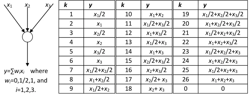
Instead of the absolute information flow on links, a chromosome in the new GA records the relative

information flow, i.e., an integer k, whose meaning is a certain predefined combination of signals on incoming links of a node. For instance, Fig.2 shows an illustration of how to predefine k. In this figure, a table is set up to define all possible signal combinations at a node with three incoming links, and the field

size is NW=3. A different number of incoming links requires a different predefined table for k, as

illustrated in Fig.3.

Let head(i) denote the serial number of the starting node of link i. It is assumed that the source has as many incoming links as there are signals to be sent, and each signal is associated with one and only one of

such assumed links. Let the gene g(i) be associated with link i. Then g(i)=k, k=0,1,…, _WnIn(head(i))

N , where

nIn(head(i)) is the number of incoming links to node head(i) . In other words, for an outgoing link, e.g.,

link i, the number of possible signal combinations (including no coding) is _NWnIn(head(i))_{. The exact}

combination that a value of k stands for needs to be predefined. Hereafter, the value of g(i) is called the

state of link i. Then the set of possible states for link i is x1 x2 x3

y=∑wixi where wi=0,1/2,1, and

i=1,2,3.

k y

1 x1/2

2 x1

3 x2/2

4 x2

5 x3/2

6 x3

7 x1/2+x2/2

8 x1+x2/2

9 x1/2+x2

k y

10 x1+x2

11 x1/2+x3/2

x1

12 x1+x3/2

13 x1/2+x3

14 x1+x3

15 x2/2+x3/2

16 x2+x3/2

17 x2/2+ x3

18 x2+ x3

k y

19 x1/2+x2/2+x3/2

20 x1+x2/2+x3/2

x1

21 x1/2+x2+x3/2

22 x1+x2+x3/2

23 x1/2+x2/2+x3

24 x1+x2/2+x3

25 x1/2+x2+x3

26 x1+x2+x3

0 0

ΘS(i)={0,1,…,

)) ( (headi n W

In

N }. (8)

Therefore, the size of the solution space of the new GA is

l In n

i

i head n W

SP N

n

1

)) ( (

. (9)

Unlike the absolute information flow on links, the states in ΘS(i) only depend on the network topology

and the number of signals that are to be sent, which are both fixed during a GA run. Therefore, as long as

g(i) remains within ΘS(i) during the evolutionary operation, there will be no feasibility problem. As will

be discussed in the following subsection, this condition is very easily fulfilled. On the other hand, the

GA. The simple illustration in Fig.3 illustrates how to use relative information flow on links to construct a

chromosome.

The new chromosome is an integer vector with of size nl. One may also use an nl×max(nIn(i)) matrix to

record the weights applied to each of the incoming links, and such a matrix representation will need no

predefined tables. In this study, we choose the vector representation because: (i) it has a lower memory

demand, particularly in the case of large-scale networks and (ii) it is more efficient in terms of algorithm

execution (the matrix representation needs to generate nIn(head(i)) random numbers to determine the

relative information flow on link i, whilst the vector representation requires only one random number). However, for networks where a node may have many incoming links, the predefined tables for the vector

representation will become unfeasibly large if the field size is also large. For instance, assuming

max(nIn(i))=10 and NW=10, then the largest predefined table will have 1010 entries for k. In this case, we

can transform the network into an equivalent network which has a relatively small max(nIn(i)), which can

actually be just 2, as illustrated in Fig.4. Then, even if NW=100, the largest predefined table only needs

1002=104 entries for k. The transformed network will have more links than the original network, which means that, according to Eq.(9), the entire search space will increase, which will become of particular

concern in the case of large-scale networks. Therefore, network decomposition methods may be employed

here as is the case in many decentralized/distributed algorithms [13].

It should be noted that the search space given by Eq.(8) and Eq.(9) is much larger than those in

x1 x2 x3

y1 y2 y3

x1 x2 x3

y1 y2 y3

previous studies. For instance, the search space size for link i is ₂nIn(head(i)) _{in [2], and even down to} nIn(head(i))+2 in [11] and [12]. Fortunately, as will be explained in Section IV, this disadvantage can be

compensated by introducing some new problem-specific heuristic rules based on the exact information

flow on links. The new rules would be difficult to apply to previous chromosome structures such as in [11]

and [12] where the exact link information flow is elusive. Actually, as will be shown in the simulation

results, the new GA reported in this study can almost always find theoretically optimal solutions, despite

the extremely large search space.

It should also be noted that the new chromosome structure depends on knowledge of the entire network

topology, which may change in the DNCP. Therefore, the new GA cannot achieve the robustness defined

by random network coding. Fortunately, the new chromosome structure may still deliver a robust

performance. This is because a specific coding scheme is defined by a chromosome in the new structure,

and it is known whether an incoming link will contribute to a coding instance or not. Therefore, when a

non-contributing incoming link is disconnected, there will be no need to re-run the optimization. In other

words, a solution based on the new chromosome structure is robust against any changes in

non-contributing incoming links. Even if a contributing incoming link is disconnected, one can easily

check whether or not there exists any non-contributing incoming link which can replace the disconnected

link, because the exact information flow on links are available thanks to the new chromosome structure.

For example in Fig.2, when k=10 (y=x1+x2) performance is not affected by the disconnection of the link

carrying x3. Alternatively, given x2=x3, then by switching to the link carrying x3,the performance when

k=10 is robust against the disconnection of the link carrying x2. This is impossible for the chromosome

structures in [11] and [12], where coding always involves all incoming links without specifying any of

their contributions. Therefore, the new chromosome structure proposed in this paper enables the resulting

GA to run in a more efficient and robust way in dynamic environments. As shown in Fig.5 (a), every time

when the network topology changes, a re-run after a re-calculation of the achievable target rate is needed

there is no need to re-calculate the target rate. Moreover, if only non-contributing incoming links are

disconnected or a replacement exists for a disconnected contributing incoming link then there is no need to

re-run the optimization. Furthermore, by minimizing the number of coding links, the above robustness

associated with the new chromosome structure can be improved because the number of non-contributing

incoming links may be increased.

C. Evolutionary Operators

The mutation operator in this paper is designed as follows. A chromosome is chosen for mutation at a

specified probability. Then a gene associated with a potential coding link needs to be chosen randomly.

When gene g(i) is chosen, the associated link is the ith link in the network with a set of possible states given by ΘS(i) as defined in Eq.(8). Mutation will randomly choose a value from the set ΘS(i)-{g(i)}, and

then reset g(i) to the new value. Thanks to the new chromosome structure, ΘS(i) depends only on the

Yes Calculate the achievable target

rate based on the current network topology.

Optimize network coding resources accordingly.

No

Yes (a) Apply existing GAs to the DNCP

Optimize network coding resources based on the current network topology.

No

(b) Apply the new GA to the DNCP

Yes No

No

Yes

Switch to replacement link(s). Does the network

topology change?

Does the network topology change?

Is any contributing incoming link disconnected?

Does any replacement link

exist?

network topology, which is fixed during a GA run meaning that the above mutation operation is free of

feasibility problems.

This paper adopts uniform crossover, which is highly efficient not only in identifying, inheriting and

protecting common genes but also in terms of re-combining uncommon genes [23], [24]. Simply

speaking, in uniform crossover, each gene of an offspring chromosome inherits the associated gene from

its two parent chromosomes with a 50% chance. In the proposed chromosome structure, the ith genes of all chromosomes share the same set (ΘS(i)) of possible states for link i. Therefore, uniform crossover will

cause no feasibility problems. Regarding the choice of two parent chromosomes, any chromosome in an

old generation may be chosen as the first parent chromosome at a fixed probability of pc, .Then a different

chromosome may be chosen as the second parent chromosome with a probability proportional to its

fitness. In this way, every chromosome stands the same chance of becoming the first parent, while a fitter

chromosome stands a better chance to cross over with most other chromosomes. This is analogous to a

dominant male mating with most females in its territory.

D. Heuristic Rules

It is well known that heuristic rules, particularly problem-specific ones, often play an important role in

the successful applications of GAs. Thanks to the new chromosome structure proposed in subsection III.B,

here we can easily integrate the following NCP-specific rules in our new GA.

Rule 1: All evolutionary operations only apply to the outgoing links of PCNs.

Rule 2: When initializing the first generation, a certain proportion of chromosomes will allow coding

on all PCNs, and for a PCN which has multiple outgoing links, choose at least one link

randomly as a coding link. This rule can help to find a solution to achieve the target rate, if it is

achievable, at all sinks.

Rule 3: Furthermore, in the initialization of the first generation, another proportion of chromosomes

actually achieved at the minimum cost of resources. It should be pointed out that this rule can

hardly hit any optimal solution by chance, because even in a network where the optimal solution

requires no coding, most no-coding schemes are not optimal.

Rule 4: In either initialization or evolutionary operations, the states of incoming links of a PCN should

be determined in such a way that the node will receive as many different signals as possible. In

other words, the signals to a PCN should be diversified as much as possible. This rule will allow

as many choices as possible for coding schemes, and therefore can help to diversify a

generation.

Rule 5: For a PCN with multiple outgoing links, there should be a high probability that the outgoing

links have different states.

Rule 6: When initializing the first generation at time instant t+1, a certain proportion of chromosomes will inherit the best solution found by the GA at time instant t. This rule is introduced particularly for the DNCP, where, although the network topology changes randomly over time,

it is reasonable to assume that there is likely to be a certain consistency in it at two successive

time instants. Therefore, inheriting the best solution found at time instant t could be very helpful to the GA in finding a good solution at time instant t+1.

It should be noted that the practicability of Rules 4 and 5 relies on the availability of exact information

flow on links. Thus the chromosome structures in [2], [11], [12] and [13] do not support these rules as they

lack this information but thanks to our new chromosome structure, it becomes possible to integrate them

into our algorithm. In the new GA, the following procedure is employed to apply Rule 4 for improving up

to one gene in a chromosome. By repeating the procedure, more genes in the chromosome can be

improved. A similar procedure is used to apply Rule 5, where outgoing links, rather than incoming links,

of PCNs will be considered, and Step 4 will be executed with a specific probability, e.g., 50% in our

experiments.

Step 2: Check if there is an unmarked PCN which has at least two incoming links carrying the same

signal. If there is no such unmarked PCN, stop.

Step 3: For the current PCN, among its incoming links which have the same signal, check if there exists

at least one link which may receive a signal different from those that the current PCN has

already received. If there is no such link, mark the current PCN, and then go to Step 2.

Step 4: For the current PCN, among its incoming links which have the same signal, randomly choose a

link which can bring new signals to the current PCN. Randomly assign such a new signal to that

link, modify the associated gene in the chromosome and then stop.

IV. SIMULATION RESULTS

A. The setup of the experiments

Firstly, the new GA was compared with three existing algorithms for the SNCP, namely the GA

reported in [2] (denoted as GA[2]), and two minimal approaches reported in [4] and [5] (denoted as

Minimal 1 and Minimal 2, respectively) to ascertain if the new algorithm can achieve similar or better

performance. Then the new GA was tested on the DNCP by applying it to problems where the

theoretically optimal solutions are known a priori to determine how close the best results generated by the new algorithm are to such theoretically optimal solutions.

In the experiments on the SNCP, there were two sets of test cases, taken from [2] for comparative

purposes. The networks in Set I were actually generated by the algorithm in [25], which constructs

connected acyclic directed graphs uniformly at random. Two networks with parameters (20 nodes, 80

links, 12 sinks, rate 4) and (40 nodes, 120 links, 12 sinks, rate 3), denoted as SCase 1 and SCase 2, were

used for simulations in Set I. The networks in Set II were constructed by cascading a number of copies of

network (c) in Fig.1 such that the source of each subsequent copy of network (c) in Fig.1 was replaced by

an earlier copy’s sink. Set II had 4 networks, which used fixed-depth binary trees containing 3, 7, 15 and

SCase 6, and they have a maximum multicast rate of 2, which is achievable without coding, i.e., the

optimal solutions have no coding links at all. Table I provides more details about these SNCP networks,

and Fig.6.(a) illustrates how SCase 3 is constructed.

Fig.6. Some examples of networks used in the experiments.

There has been no directly comparable work to this published to date for DNCP algorithms. Therefore,

to conduct experiments on the DNCP, appropriate test cases needed to be designed where the theoretically

optimal solutions to the DNCP were known a priori, so that the performance of the new GA could be precisely assessed. All DNCP test cases in this paper were designed based on Set II of the SNCP networks.

In contrast to static networks, where all links remained for the duration of the simulation, in the DNCP test

cases, links were introduced that could be disconnected and reconnected dynamically. At each time

instant, the dynamic links that were to be disconnected and/or reconnected were randomly chosen. In TABLEI

NETWORKS USED IN DIFFERENT SNCPTEST CASES Copy the network Fig.1.(c)

Or generated by [24]

Nodes Links Sinks Target rate SCase 1 Generated by [24] 20 80 12 4 SCase 2 Generated by [24] 40 120 12 3 SCase 3 3 copies of Fig.1.(c) 19 30 4 2 SCase 4 7 copies of Fig.1.(c) 43 70 8 2 SCase 5 15 copies of Fig.1.(c) 91 150 16 2 SCase 6 31 copies of Fig.1.(c) 187 300 32 2

(a) How to construct the network of SCase 3 (b) An example of dynamic networks with link replacement

of Category I (DCase 1)

(c) An example of dynamic networks with link replacement

of Category II (DCase 5)

(d) An example of dynamic networks with link replacement

of Category III (DCase 9)

Dynamic link which can randomly disconnect and reconnect

Constant link Disconnected dynamic link

order to be able to derive the theoretically optimal solutions for a dynamic network at any time instant,

only a few constant links in the SNCP networks were replaced by dynamic links in the DNCP test cases. In

this study, three categories of link replacements were considered so that the results accounted for different

degrees of complexity. Based on the 4 SNCP test cases, 4 DNCP test cases were constructed for each

category of replacement. Therefore, there were 12 DNCP test cases, whose main features are summarized

in Table II.

In Category I, for every copy of network (c) in Fig.1, a permanent link between node 4 and node 5 in

network (c) was replaced by a dynamic link, as illustrated in Fig.6.(b). It can be seen that this category of

replacement did not affect the theoretically maximal network throughput (TMNT). This is because, when

the dynamic link in a copy of network (c) of Fig.1 was disconnected, the original TMNT could be

achieved by coding at node 4 of that copy. Therefore, in a Category I dynamic network with link

replacement, no matter how the dynamic links were disconnected and reconnected, the TMNT remained

the same as if all dynamic links were connected, i.e. the theoretical maximal achievable rate (TMAR) at

each sink was always 2. The TMNT here can be calculated as 2×ns. An optimal solution to achieve the

TMNT is: coding at node 4 of a copy only if the associated dynamic link is disconnected. In other words,

the minimal number of coding nodes/links in the optimal solution, i.e., the theoretically minimal number

of coding links (TMNCL) at time instant t, is equal to nDDL(t), the number of disconnected dynamic links

TABLEII

MAIN FEATURES OF 12DNCPTEST CASES DNCP Case Based on

which SNCP Case

Category of Link Replacement

Number of Dynamic

Links

TMNT TMNCL

DCase 1 SCase 3 I 3 _{2×ns nDDL(t)} DCase 2 SCase 4 I 7 _{2×ns nDDL(t)} DCase 3 SCase 5 I 15 _{2×ns nDDL(t)} DCase 4 SCase 6 I 31 2×ns nDDL(t) DCase 5 SCase 3 II 6 2×ns-nDS(t) 0 DCase 6 SCase 4 II 14 _2×ns-nDS(t) 0 DCase 7 SCase 5 II 30 _2×ns-nDS(t) 0 DCase 8 SCase 6 II 62 _2×ns-nDS(t) 0 DCase 9 SCase 3 III 9 _{2×ns-nDS(t) n (t)}

DDL

DCase 10 SCase 4 III 21 _{2×ns-nDS(t) n (t)}

DDL

DCase 11 SCase 5 III 45 _{2×ns-nDS(t) n (t)}

DDL

at time instant t.

In Category II, for every copy of network (c) in Fig.1, the constant links between node 2 and node 6,

and node 3 and node 7 in network (c) were replaced by dynamic links, as illustrated in Fig.6.(c). Clearly,

when a dynamic link was disconnected, the TMAR at every one of its downstream sink(s) decreased to 1,

regardless of network coding. The TMNT at time instant t can be calculated as 2×ns-nDS(t), where nDS(t) is

the number of downstream sinks of disconnected dynamic links at time instant t. The TMNT can be achieved with no coding, which means the TMNCL is always zero.

Category III was actually a combination of Category I and Category II, as illustrated in Fig.6.(d). With

this category of link replacement, both the TMNT and the TMNCL were dependent on how the dynamic

links were disconnected and reconnected. Fortunately, it was quite straightforward to derive the TMNT

and the TMNCL of a dynamic network with link replacement of Category III by using the following rules.

First, if the dynamic link between node 2 and node 6 (or node 3 and node 7) of a copy was disconnected,

then the TMAR of every downstream sink of this disconnected link was 1, and no coding or further

analysis needed to be applied to its downstream tree. Second, subject to the first rule, if all downstream

sinks of the left/right tree of a copy had a TMAR of 1, then no coding was necessary at node 4 of the copy.

Third, subject to the above two rules, if the dynamic link between node 4 and node 5 of a copy was

disconnected, an optimal solution required coding at node 4. The TMNT at time instant t was 2×ns-nDS(t),

as in Category II, while the TMNCL at time instant t was equal to nDDL(t), the number of disconnected

dynamic links as described in Rule 3.

To investigate whether the heuristic rules reported in Section III.D really worked, three versions of the

new GA were used in the experiments. The first version, denoted as GA1, only employed Rule 1 and Rule

2, the second version, denoted as GA2, used Rules 1, Rule 2 and Rule 3, and the third version, denoted as

GA3, adopted Rule 1 to Rule 5. In GA1 to GA3, the mutation probability and crossover probability were

0.1 and 0.4, respectively. The population size and upper bound for the number of generations for evolution

the next generation directly. In each generation, 15 chromosomes were generated randomly with no link to

the previous generation, in order to maintain the diversity in the new generation. The coefficients in the

fitness function given by Eq.(5) to Eq.(7) were α1=α2=10, α3=1, α4=0, α5=200 and α6=0. For the sake of

simplicity, in most experiments w(i,j,h)=0 or 1 in Eq.(4), i.e., the field size was NW=2, unless specified

otherwise. In each test case, 20 random experiments were conducted for each algorithm and the network

changed randomly 50 times in each DNCP test case. The average results of the experiments follow in the

following subsections including statistical analysis (standard deviations (SD) and Kruskal-Wallis tests

[26]) for GA1 to GA3. Variations in the results are revealed by the calculation of the former, whilst the

latter enables the determination of the significance of the performance differences between GA1, GA2 and

GA3. In each Kruskal-Wallis test, the significance of the difference between the performances of GA1 and

GA2, GA1 and GA3, and GA2 and GA3 was measured by the value of the occurrence probabilities p12, p13

and p23 for the respective pairwise comparisons, with a value smaller than 0.05 indicating a statistically

significant difference. However, due to the limited space, the SD values are only listed in Table IV, Table

V and Table VII; Only Table IV includes the results of Kruskal-Wallis tests in order to give readers an

idea what p12, p13 and p23 could be like, and in other experiments, the results of Kruskal-Wallis tests are

just summarized in the associated discussions.

B. The experimental results of SNCP

The average experimental results of the static cases are listed in Table III, and Table IV reveals more

details about the performance of GA1 to GA3. From these results one can make the following

observations:

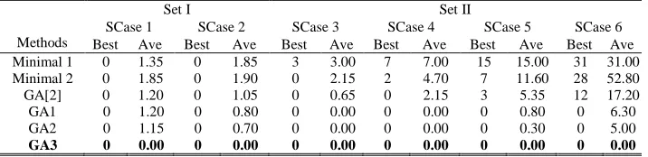
Table III shows that, in the cases of Set I, all the methods perform similarly. In more precise terms, the

GAs reported in this paper, i.e., GA1, GA2 and GA3, return slightly lower average numbers of coding

links than the existing methods. However, since all methods can find the optimal (i.e., no coding

algorithm has a significant advantage when compared with existing algorithms. Analysis of the

network topologies in Set I suggests that these networks have too many links; for one network, nl=4nn,

and for the other, nl=3nn. In the Graph Drawing Community, graphs (i.e., networks) having nl=4nn

links are actually considered to be dense [25]. In such a network with dense links, it is easy to achieve

a relatively small target rate without network coding. Compared with Set I, all the networks in Set II

have nl<2nn. Therefore, although the target rates in Set II are smaller than those in Set I, it is probably

more difficult to find a no-coding solution to achieve the smaller target rates in Set II. Actually, in the

Set II cases, the results of a comparison of these methods show significant differences, which may

suggest that the networks in Set II are more suitable for testing different methods. Therefore, hereafter,

we will only focus on analyzing the results of SCase 3 to SCase 6.

TABLEIII

RESULTS OF SNCPSIMULATIONS (NUMBER OF CODING LINKS)

Methods

Set I Set II

SCase 1 SCase 2 SCase 3 SCase 4 SCase 5 SCase 6 Best Ave Best Ave Best Ave Best Ave Best Ave Best Ave Minimal 1 0 1.35 0 1.85 3 3.00 7 7.00 15 15.00 31 31.00 Minimal 2 0 1.85 0 1.90 0 2.15 2 4.70 7 11.60 28 52.80 GA[2] 0 1.20 0 1.05 0 0.65 0 2.15 3 5.35 12 17.20 GA1 0 1.20 0 0.80 0 0.00 0 0.00 0 0.80 0 6.30 GA2 0 1.15 0 0.70 0 0.00 0 0.00 0 0.30 0 5.00

GA3 0 0.00 0 0.00 0 0.00 0 0.00 0 0.00 0 0.00

Table III also shows that for Set II GA1, GA2 and GA3 clearly outperform the existing algorithms,

which struggle to find the theoretically optimal solutions, particularly in complicated cases such as

SCase 5 and SCase 6. All three new GAs are capable of finding the theoretically optimal solutions in

all 6 SNCP cases, with GA3 always finding the theoretically optimal solutions.

Since GA1 adopts exactly the same heuristic rules as the GA in [2] but displays superior performance,

particularly in SCase 5 and SCase 6 suggesting that the GA designs here are more suitable for the

NCP than the GA designs in [2].

On average, GA2 achieves a better performance than GA1 and the former has one more heuristic rule

(Rule 3) it is reasonable to assume that the performance improvement is due to that rule. Moreover, as

algorithm would also be improved by Rule 3. However, when one examines the p12 in the

Kruskal-Wallis test, the values are much greater than 0.05 in each case, so there is no statistically

significant difference between the performance of GA1 and GA2 and the advantage of Rule 3 is

minor.

TABLEIV

DETAILS OF THE RESULTS OF THE NEW GAS (20RUNS FOR EACH CASE)

(Average results of 20 runs) SCase 1 SCase 2 SCase 3 SCase 4 SCase 5 SCase 6 Mean SD Mean SD Mean SD Mean SD Mean SD Mean SD Final max fitness

GA1 149.65 45.51 190.00 57.98 240.00 0.00 240.00 0.00 181.67 63.46 40.21 35.06 GA2 171.54 42.97 195.66 48.30 240.00 0.00 240.00 0.00 195.64 76.24 59.09 29.14

GA3 280.00 0.00 260.00 0.00 240.00 0.00 240.00 0.00 240.00 0.00 240.00 0.00

How many generations to achieve final max

fitness

GA1 245.50 58.21 239.60 115.21 2.35 1.94 9.40 3.78 242.40 85.77 300.00 0.00 GA2 210.75 53.06 221.00 102.24 1.05 0.24 5.80 10.20 171.90 129.47 300.00 0.00

GA3 64.40 18.96 39.10 13.83 1.00 0.00 2.20 1.03 11.45 5.89 56.70 38.15

Average minimal coding links

GA1 1.20 0.79 0.80 0.92 0.00 0.00 0.00 0.00 0.80 1.03 6.30 7.09 GA2 1.15 1.10 0.70 0.48 0.00 0.00 0.00 0.00 0.30 0.67 5.00 3.86

GA3 0.00 0.00 0.00 0.00 0.00 0.00 0.00 0.00 0.00 0.00 0.00 0.00

Maximum minimal coding links

in all tests

GA1 4 3 0 1 3 22

GA2 3 1 0 0 2 12

GA3 0 0 0 0 0 0

Minimum actually achieved rate at sinks in all tests

GA1 3 3 2 2 1 1

GA2 3 3 2 2 2 1

GA3 4 3 2 2 2 2

Kruskal-Wallis test results

p12 0.78 0.91 1.00 1.00 0.82 0.62

p13 0.00 0.00 1.00 1.00 0.01 0.00

P23 0.01 0.01 1.00 1.00 0.02 0.00

Table III and Table IV show that GA3 is the best algorithm of all, its advantages are confirmed by the

associated Kruskal-Wallis test results, which are smaller than 0.05 in all static cases except the

simplest (SCase 3 and SCase 4) where GA1 and GA2 can often find the optimal solutions. It should

be noted that the theoretical maximum fitness is 240 for SCase 3 to SCase 6. Table IV shows that GA3

always achieves this maximum fitness within 300 generations of evolution (as the associated SD

values are zero). From this table, one can see that GA3 converges much more quickly than GA1 and

GA2, always finding the theoretical optimal solutions. Since the only difference between GA3 and

GA2 is the integration of Rule 4 and Rule 5 into GA3, it is reasonable to conclude that it is the impact

of these two additional rules that play a significant role in improving the performance of the GA. As

mentioned in Section III.D, it is the new chromosome structure that makes it possible to integrate

these two rules into the new GA. It should be noted that Rule 4 and Rule 5 are not designed solely for

Therefore, one may say that the new chromosome structure exhibits some advantages as compared

with the binary matrix representations used in [2], [11], [12] and [13], where Rule 4 and Rule 5 are not

applicable.

C. The experimental results of DNCP

With the 12 DNCP test cases, the performances of GA1 to GA3 can be assessed easily by comparing the

actually achieved network throughput (AANT) and the actually minimal number of coding links

(AMNCL) with the TMNT and the TMNCL. Besides examining the gap between the actually achieved

values and the theoretical ones, it is also important to determine how many times the GA has found the

optimal solutions, which is reflected by the convergence rate (CR). The closer the CR is to 1, the better the

performance of the GA. The experimental results are given in Table V, from which one can see that:

In all DNCP test cases, the values actually achieved by GA3 are very close to the theoretical values, and

the CR is close to 1. This implies that, in the dynamic environment, GA3 can still converge to the

theoretically optimal solutions, regardless of any random changes in the network topology so we can

conclude that the GA developed in this paper is very effective at resolving the DNCP.

In a similar way to the static experiments, GA1 to GA3 have almost the same performance in the simple

test cases, i.e., DCase 1, DCase 2, DCase 5, DCase 6, DCase 9 and DCase 10. In the complicated test

cases, the overall performance of GA2 is better than that of GA1, i.e., the AANTs of GA2 are generally

TABLEV

RESULTS OF THE DNCPTESTS

(Ave. results of 20 exp.) TMNT AANT TMNCL AMNCL CR

GA1 GA2 GA3 GA1 GA2 GA3 GA1 GA2 GA3

Mean SD Mean SD Mean SD Mean SD Mean SD Mean SD Link

replacement of Category I

DCase 1 8.00 8.00 0.00 8.00 0.00 8.00 0.00 1.00 1.00 0.00 1.00 0.00 1.00 0.00 1.00 1.00 1.00

DCase 2 16.00 16.00 0.00 16.00 0.00 16.00 0.00 2.00 2.50 2.63 2.25 2.37 2.00 0.00 0.75 0.75 1.00

DCase 3 32.00 31.00 1.15 31.25 1.50 31.75 0.50 4.25 5.00 4.24 4.50 4.78 4.00 4.08 0.25 0.50 0.75

DCase 4 64.00 55.05 2.45 56.25 5.19 62.50 2.98 9.00 10.25 3.09 7.25 5.25 6.80 7.41 0.00 0.00 0.35

Link replacement

of Category II

DCase 5 7.00 7.00 0.00 7.00 0.00 7.00 0.00 0.00 0.00 0.00 0.00 0.00 0.00 0.00 1.00 1.00 1.00

DCase 6 14.75 14.75 0.00 14.75 0.00 14.75 0.00 0.00 0.00 0.00 0.00 0.00 0.00 0.00 1.00 1.00 1.00

DCase 7 28.50 28.50 0.00 28.50 0.00 28.50 0.00 0.00 0.00 0.00 0.00 0.00 0.00 0.00 1.00 1.00 1.00

DCase 8 58.00 55.75 4.27 54.00 58.00 0.00 0.00 3.50 0.25 0.75 1.50 0.00 0.00 0.25 0.30 1.00

Link replacement

of Category III

DCase 9 6.25 6.25 0.00 6.25 0.00 6.25 0.00 0.00 0.00 0.00 0.00 0.00 0.00 0.00 1.00 1.00 1.00

DCase 10 12.75 12.75 0.00 12.75 0.00 12.75 0.00 1.00 1.00 0.00 1.00 0.00 1.00 0.00 1.00 1.00 1.00

DCase 11 23.50 22.35 8.01 23.50 0.00 23.50 0.00 0.25 3.25 4.05 0.25 0.00 0.25 0.00 0.70 1.00 1.00

larger than, or similar to, those of GA1; the AMNCLs of GA2 are smaller than those of GA1, and the

CRs of GA2 are larger than those of GA1. There is also a significant increase in performance between

GA2 and GA3 in the complicated dynamic test cases. These results again confirm the importance of

Rule 3 to Rule 5. In the Kruskal-Wallis tests for DCase 4, DCase 8 and DCase 12, the three most

complicated test cases, p12 is larger than 0.05, whilst both p13 and p23 are smaller than 0.05. Therefore,

it may be concluded that Rule 3 does not bring any statistically significant improvement, whilst Rule 4

and Rule 5 are highly effective in the DNCP.

It is worthwhile reminding the reader that the main aim of this DNCP study is to investigate the

performance of our GAs in the situation where the target rate may become theoretically unachievable.

Therefore any method which is based on the assumption that the target rate is achievable will not be

easy to apply. There are many other important issues in the DNCP, such as uncertainties, robustness

and time delay that remain to be addressed in future work because the DNCP remains a largely

unexplored area in network coding research. Therefore, further extensive investigative effort is

required to develop research relating to the DNCP.

One may notice that in Table V, the average AMNCL is sometimes smaller than the average TMNCL.

This is because the TMNCL is the minimal coding links required to achieve the TMNT, whilst the GAs

sometimes converged to a solution which does not achieve the TMNT but uses fewer coding links than

the TMNCL.

D. Further analysis of Rule 4 and Rule 5

As has been emphasized throughout this paper, one major contribution of our reported GAs as compared

with other existing GAs for the NCP is the new chromosome structure, which makes it possible to

calculate the exact information flow on links and therefore facilitates the integration of new

problem-specific heuristic rules, particularly Rule 4 and Rule 5 into the system. To further verify this

contribution, the roles played by Rule 4 and Rule 5 will be examined in more detail in this subsection. For

most difficult static case. In all previous experiments, when the focus was to improve a chromosome, GA3

applied Rule 4 and Rule 5 no more than once. In other words, GA3 used Rule 4 and Rule 5 to modify no

more than one gene of a chromosome. In this subsection, GA3 is allowed to apply Rule 4 and Rule 5 to

modify up to NR4R5 genes of a chromosome, where NR4R5=1,…,10. All other algorithm related parameters

remain the same as in previous experiments.

The results are given in Table VI, from which the following observations can be made. GA3 can always

find the theoretical optimal solutions, while GA1 and GA2 often struggle to do so and so we state that Rule

4 and Rule 5 are the cause of the advantages and that applying them more times leads to better

performance since the using a larger NR4R5 means that GA3 needs fewer generations to converge.

However, applying these rules causes an additional computational burden producing longer computation

times for a generation of GA3 than for GA1 and GA2. Fortunately, when we combine the computational

time consumed by a generation and the generations needed to converge to the optimal solutions, it

becomes clear that the total computational time consumed by GA3 to find the optimal solutions is actually

smaller than those of GA1 and GA2. Considering the influence of NR4R5 on the total computational time of

GA3, it seems a balance should be made to set up NR4R5 because the smallest total computational time

occurs with a medium sized NR4R5. In the case of SCase 6, the best value for NR4R5 is 8, which results in

GA3 being able to find the optimal solutions at the fastest speed.

Hence it may be concluded that GA3 out performs GA1 and GA2 in terms of not only the quality of the

solution but also in terms of computational efficiency. This shows that the introduction of Rule 4 and Rule

5 is very advantageous and hence justifies the use of the new chromosome structure as proposed in this

paper.

TABLEVI

COMPUTATIONAL EFFICIENCIES OF DIFFERENT GAS BASED ON SCASE6

(Ave. results of 20 exp.) GA1 GA2 GA3 with a NR4R5 of

1 2 3 4 5 6 7 8 9 10

Final max fitness 40.21 59.09 240.00 240.00 240.00 240.00 240.00 240.00 240.00 240.00 240.00 240.00

Number of coding links 6.30 5.00 0.00 0.00 0.00 0.00 0.00 0.00 0.00 0.00 0.00 0.00

Generations to converge 300.00 300.00 56.70 28.40 15.60 11.10 4.30 3.90 3.40 3.00 3.00 2.70

Computational time of one generation (sec.)

time (sec.)

E. The influence of field size on the performance of our new GAs

It is well known that a large enough field size plays a crucial role in achieving the maximum possible

throughput. However, Eq.(8) shows that, in the case of our new GAs, the search space size for a single

outgoing link will grow exponentially with the field size, which implies that a larger field size might make

it more difficult for our new GAs to find even good solutions. Therefore, the focus of this subsection is to

explore and examine the influence of field size on the performance of our new GAs. Five field sizes,

NW=2, 4, 6, 8 and 10, were used in GA1, GA2 and GA3 with NR4R5 set to 8 for GA3 based on the above. To

maintain this work at a reasonable length, the networks used in this experiment were those static cases in

Set II, and only the average results for the final max fitness and total computational time are given in Table

VII.

From the table, several observations can be made. The field size has a significant influence on the

performance of GA1. In the case of SCase 3, the simplest network of all, GA1 with a different field size

can always find the optimal solutions but it takes more time when a larger NW is adopted. In the case of

SCase 4 and SCase 5, GA1 may still find the optimal solutions when NW is small, but the solution quality

reduces quickly as NW increases. In SCase 6, the most complex network of all, GA1 struggles and usually

can only find feasible solutions, regardless of the value of NW. It can be seen in Table VII that the

influence of field size on the performance of GA2 is similar to its influence on GA1. The only difference is

that GA2 performs a little better than GA1 in the simple cases. In the case of SCase 6, GA2 has almost the

same performance as that of GA1, regardless of the value of NW. In all test cases, in terms of either

solution quality or computational time, GA3 has a very robust performance against the change of NW.

Actually, for a given network, GA3 can always find the optimal solution with similar computational time,

no matter what value NW has. In the associated Kruskal-Wallis tests, p12 is usually larger than 0.05 (except

in SCase 4 with NW ≥6), which means the performances of GA1 and GA2 are statistically the same; p13 is