http://wrap.warwick.ac.uk
Original citation:
Elliott, Mark T., Wing, A. M. and Welchman, A. E.. (2014) Moving in time :
Bayesian
causal inference explains movement coordination to auditory beats. Proceedings of the
Royal Society B: Biological Sciences, Volume 281 (Number 1786). Article number
20140751. ISSN 0962-8452
Permanent WRAP url:
http://wrap.warwick.ac.uk/66131
Copyright and reuse:
The Warwick Research Archive Portal (WRAP) makes this work of researchers of the
University of Warwick available open access under the following conditions.
This article is made available under the Creative Commons Attribution 3.0 (CC BY 3.0)
license and may be reused according to the conditions of the license. For more details
see:
http://creativecommons.org/licenses/by/3.0/
A note on versions:
The version presented in WRAP is the published version, or, version of record, and may
be cited as it appears here.
rspb.royalsocietypublishing.org
Research
Cite this article:
Elliott MT, Wing AM,
Welchman AE. 2014 Moving in time: Bayesian
causal inference explains movement
coordination to auditory beats.
Proc. R. Soc. B
281
: 20140751.
http://dx.doi.org/10.1098/rspb.2014.0751
Received: 27 March 2014
Accepted: 16 April 2014
Subject Areas:
computational biology, behaviour,
neuroscience
Keywords:
movement synchronization, Bayesian inference,
sensory integration, motor timing
Author for correspondence:
Mark T. Elliott
e-mail: [email protected]
Electronic supplementary material is available
at http://dx.doi.org/10.1098/rspb.2014.0751 or
via http://rspb.royalsocietypublishing.org.
Moving in time: Bayesian causal inference
explains movement coordination to
auditory beats
Mark T. Elliott
1, Alan M. Wing
1and Andrew E. Welchman
21School of Psychology, University of Birmingham, Edgbaston B15 2TT, UK 2Department of Psychology, University of Cambridge, Cambridge CB2 3EB, UK
Many everyday skilled actions depend on moving in time with signals that are embedded in complex auditory streams (e.g. musical performance, dancing or simply holding a conversation). Such behaviour is apparently effortless; however, it is not known how humans combine auditory signals to support movement production and coordination. Here, we test how participants syn-chronize their movements when there are potentially conflicting auditory targets to guide their actions. Participants tapped their fingers in time with two simultaneously presented metronomes of equal tempo, but differing in phase and temporal regularity. Synchronization therefore depended on inte-grating the two timing cues into a single-event estimate or treating the cues as independent and thereby selecting one signal over the other. We show that a Bayesian inference process explains the situations in which participants choose to integrate or separate signals, and predicts motor timing errors. Simu-lations of this causal inference process demonstrate that this model provides a better description of the data than other plausible models. Our findings suggest that humans exploit a Bayesian inference process to control movement timing in situations where the origin of auditory signals needs to be resolved.
1. Introduction
Many human activities, from holding a conversation to playing music, have their basis in our ability to extract meaningful temporal structure from incoming sounds. For rhythmical structures in particular, humans identify key events and extract the underlying ‘beat’ of the auditory signals [1]. Such auditory rhythms promote movements ‘in time’ with the beat with little apparent effort [2,3], as demonstrated through the capacity to dance or play along to music com-prising multiple rhythmic streams. Yet, for such complex stimuli, it is unknown how temporal events are extracted and chosen as the targets to which movements are synchronized.
The complexity of incoming auditory signals is partially reduced by early sensory processing that filters out irrelevant auditory information [4]. Neverthe-less, auditory signals of interest may still consist of multiple components. For instance, keeping in time with other players in a quartet involves sensing differ-ent sequences of tones (e.g. the notes played on the viola versus cello) that share an underlying rhythm but are likely to fluctuate in relative phase, depending on how well each player can remain in time with the rest of the group [5]. Based on these discrepancies, the brain must determine whether to integrate relevant components into a single stream or treat them as separate [6].
In multisensory settings, the decision to integrate cues or treat them as separ-ate sources is well captured using the Bayesian framework of causal inference [7–10], based on the statistical probability that sensory events relate to a single event in the environment versus multiple events. If there is evidence that sen-sations originate from a single environmental cause, the sensory cues are combined in a statistically optimal way across modalities to gain the best estimate of an object or event [11–13]. Within a single modality, there is also evidence for
statistically optimal combination, for instance in combining distinct visual features such as disparity, motion or texture [14–16]. Critically, however, such integration is believed to be mandatory. Here, we test for the integration of within-modality auditory cues to time. We evaluate whether the brain applies a causal inference process to determine the cir-cumstances under which auditory sequences (distinguished only by tone frequency) should be integrated into a coherent estimate of rhythm or separated into distinct events.
First, we develop a Bayesian causal inference model for movement synchronization that describes the scenarios under which a regular stream of sensory cues from same-modality sources are integrated. Then, we test the model by asking participants to tap their index finger in time to auditory sequences that comprised two auditory metronomes presented simultaneously with equal mean tempo. To test the causal inference process, we manipulated these cues in two different ways. First, we applied a phase offset between the metro-nomes, such that the beats from one metronome occurred shortly before the other. Second, we varied the temporal reliability of the metronomes such that rather than having isochronous beat onsets, they varied randomly around the (underlying) isochronous onset time (referred to as ‘jitter’). By adding small levels of jitter to one metronome and large levels of jitter to the other, we manipulated the relative reliability of the two metronome sources [17]. Thus, we were able to observe changes in the timing and variability of partici-pants’ finger taps and assess the conditions under which the cues appeared to be integrated or treated as separate. Finally, we test four models and fit the simulated results to the exper-imental data to investigate whether causal inference best describes the observed results. We found that a causal inference model that adjusts for a consistent phase offset between cues demonstrated a fit close to the empirical data, exceeding that of alternative models based on the exclusive integration or exclusive separation of cues.
2. Material and methods
(a) Participants
Staff and students from the University of Birmingham were recruited to participate in the experiment. Participants provided informed consent and were screened for sensory and motor def-icits. Nine participants (seven male, four left-handed, mean age: 29.8+5.9 years) took part. Five participants had some musical expertise (i.e. currently play a musical instrument; mean years of experience¼10.8).
(b) Experimental set-up
Participants sat at a table wearing a pair of headphones (Sennheiser EH150) through which the auditory metronome cues were pre-sented. They tapped the index finger of their dominant hand in time to the metronome on to a wooden surface mounted on a force sensor. Responses were registered using a data acquisition device (USB-6229, National Instruments Inc., USA). Metronome presentation was controlled using the MATTAP toolbox [18].
(c) Metronome stimuli
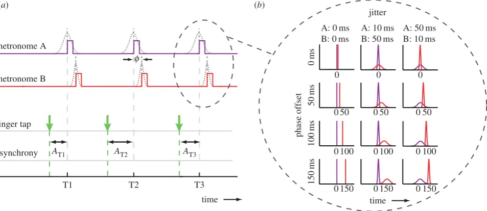
The auditory stimuli consisted of two independently controlled auditory metronomes (metronome A, pitch 700 Hz; and metro-nome B, pitch 1400 Hz; figure 1a). The metronomes were offset in phase (0, 50, 100 or 150 ms), such that metronome B followed metronome A (pilot testing established that pitch order (low–high versus high–low) did not influence synchronization behaviour). Metronome beats lasted 30 ms and the period was varied randomly (by the same amount for A and B) across trials with a value between 470 and 530 ms, to minimize learning of tempo across trials and encourage adaptive correction within trials.
To manipulate metronome reliability, we applied temporal jitter independently to each metronome (figure 1b) by perturbing the regular onset of the metronome beat by a random value sampled from a Gaussian distribution (m¼0;s¼10 or 50 ms). We tested the effect of differing reliabilities between the two metronomes and whether this would influence finger movement
finger tap
asynchrony AT1 AT2 AT3
T1 T2
f
T3 metronome B
metronome A
time A: 0 ms
B: 0 ms
A: 10 ms B: 50 ms
A: 50 ms B: 10 ms
time
(a) (b)
phase offset
50
ms
100
ms
150
ms
0 0 0
50 0
0 100
0 150
50
0 050
0 100 0 100
0 150 0 150
0m
s
[image:3.595.62.539.43.250.2]jitter
Figure 1.
(
a
) An illustration showing the timing relationships between the two metronomes and the calculation of asynchronies. The square pulses show the regular
onset time of the metronome beats (before jitter applied). Both metronomes had the same underlying period, and metronome B had a phase-offset delay from
metronome A of
f
¼
0, 50, 100 or 150 ms. To create temporal uncertainty, a random perturbation (‘jitter’) was added to the regular onset time of each beat. The
s.d. of the jitter distribution differed between metronomes (A, B:
f
0, 0 ms
g
;
f
10, 50 ms
g
;
f
50, 10 ms
g
(depicted)). Asynchronies (
A
) were calculated between the
finger-tap onsets and the onset of metronome A, before jitter was applied. (
b
) Probability distributions of metronome beat onsets. Illustration showing the expected
distributions of beat onsets relative to the regular beat onset of metronome A (0 ms). Distributions are shown for each phase offset (row) and jitter condition
(column). (Online version in colour.)
rspb.r
oy
alsocietypublishing.org
Pr
oc.
R.
Soc.
B
281
:
20140751
onsets and variability. Hence, we used the following jitter con-ditions (s.d. for metronome A and metronome B):f10, 50 msg,
f50, 10 msg and a baseline condition where both metronomes were reliablef0, 0 msg.
Participants were not explicitly informed that the auditory cues consisted of two metronomes. Instead, they were instructed to ‘tap in time to the metronome’ with some trials appearing ‘harder to tap along to than others’. This instruction was intended to encourage participants to use both cues and not attempt to ignore one in favour of the other.
Participants completed 10 trials per condition (12 conditions in all), with each trial consisting of 30 metronome beats. Con-ditions were randomized across trials to minimize any prior expectation about the metronome statistics building up across trials. To allow participants to build up prior knowledge of the metronome within a trial, analyses were performed on the tap-metronome asynchronies of beats 15–28 (the last two were ignored to discount anticipation or termination effects at the trial end [19]).
To determine baseline movement synchronization behaviour, we also presented 30 trials on which a single metronome was presented, where the degree of jitter applied was varied across trials (0, 10 or 50 ms).
(d) Analysis
To quantify synchronization behaviour, we measured the time difference between the onset of the participants’ finger taps and the metronome beat (asynchrony; figure 1a). We referenced all metronome beats relative to the onset of metronome A (prior to any jitter perturbations) to provide a consistent, static reference point for all trials regardless of condition. Negative asynchronies indicated that the finger tap preceded the onset of the beat. We calculated the s.d. of asynchronies within a trial across partici-pants and conditions. A repeated measures ANOVA was used to determine any significant effects of phase offset or jitter on the asynchrony s.d. We quantified the distribution of asynchronies for each participant, grouped by condition and tested the exper-imental data for unimodality or bimodality using Gaussian mixture models (GMMs) with either one or two centres. Mean asynchronies were then calculated based on the best fitting GMM distribution.
For comparison with the simulated asynchrony distributions of the models we tested, we fit the empirical data with probability density functions (PDFs). These were estimated using a Gaussian kernel density estimator (KDE) [20] method implemented in
MATLAB[21].
(e) Sensorimotor synchronization based on a causal
inference model
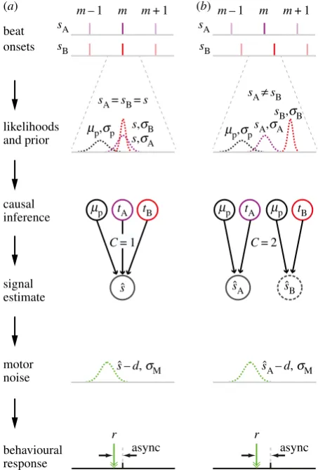
Here, we outline the features of the simulated task where an observer uses Bayesian causal inference to synchronize their movements. An overview is shown schematically in figure 2 while the full model derivation is provided in the electronic supplementary material, A.
The observer’s task is to synchronize their movements to rhythmic auditory cues presented to them. The cues consist of two discrete tones of different pitch (sA and sB). The observer
must estimate the onsets of the underlying beats produced by the auditory cues to make movements in synchrony with those beats. They do this using a causal inference process based on: (i) the likelihood of the onsets of the two auditory cues, whose true onset times are corrupted by sensory noise; and (ii) the prior expectation of where the beat will occur, which is based on the previous beat onset estimate [22,23]. The causal inference process allows the observer to determine whether the two audi-tory cues should form a single common beat and hence combine
beat
likelihoods and prior
sA=sB=s sAπsB
C= 1 C= 2
mp,sp
mp tA mp mp
sˆ
sˆ –d, sM sˆA–d, sM s
ˆA sˆB tB
s,sB
s,sA mp,sp
sB,sB sA,sA
causal inference
signal estimate
motor noise
r r
async async
behavioural response
sA
m– 1 m m+ 1
sB
sA
m– 1 m m+ 1
sB onsets
(a) (b)
[image:4.595.318.545.43.378.2]tB tA
Figure 2.
Schematic of the causal chain. (
a
) Common stream: signals are
generated from a common source (
s
A¼
s
B¼
s
). The sensory likelihood
distri-butions for the two metronome signals are modelled by Gaussian distridistri-butions
N
(
s
,
s
A) and
N
(
s
,
s
B), respectively, where
s
A,
s
Bdescribes the uncertainty
in the sensory registration. The observer has an expectation of where the
m
th
beat should occur, centred around a time
m
prelative to the true beat
s
. This
prior expectation is equal to the difference between their beat onset estimate
sˆ
and the true onset time
s
on the preceding (
m
2
1th) beat and is modelled
as a Gaussian distribution
N
(
m
p,
s
p), where
s
pdefines the strength of the prior.
The observer estimates the cue onset times
t
Aand
t
B, which are sampled from the
likelihood distributions. Using the information from
m
p,
t
Aand
t
B, the causal
inference process results in evidence that the signals define a common beat
(
C
¼
1), and the estimated signal onset time
sˆ
is calculated as a weighted
aver-age of
m
p,
t
Aand
t
B. The reliability of the three distributions 1/
s
2p, 1/
s
2 A
, 1/
s
2 B
defines the relative weightings. The observer plans their movement to coincide
with the estimated beat
sˆ
, introducing motor noise
s
M, and an anticipation
effect
d
, which results in the observable asynchrony between the movement
r
, and the true beat
s
. (
b
) Independent streams: two signals are generated
from independent sources (
s
Aand
s
B). The sensory estimation process is the
same as for (
a
); however, the prior is defined as the difference between their
beat onset estimate
sˆ
and the true onset time
s
Aon the
m
2
1th beat.
Based on
m
p,
t
Aand
t
B, the causal inference model has more evidence that
sig-nals are independent (
C
¼
2). Signal onset estimates
sˆ
Aand
sˆ
Bare therefore
calculated independently as the weighted average of
m
p,
t
Aand
m
p,
t
B,
respect-ively. Similarly, the relative weightings are proportional to their reliabilities,
1/
s
2p
, 1/
s
2A
and 1/
s
2 p
, 1/
s
2
B
. As the observer has two estimated signal
onsets, they select one with which to synchronize their movement. That is,
the observer will define the signal onset estimate to be either
sˆ
¼
sˆ
A(as
depicted in figure), or
sˆ
¼
sˆ
B. This choice varies for each beat, with observers’
esoteric preferences dominating the relative reliability of the two signals. The
observer plans their movement to coincide with the estimated beat
sˆ
, introducing
motor noise
s
M, and an anticipation effect
d
. This results in the observable
asyn-chrony between the movement
r
, and the referenced true beat (always
s
A, to
match experimental analyses). (Online version in colour.)
rspb.r
oy
alsocietypublishing.org
Pr
oc.
R.
Soc.
B
281
:
20140751
the likelihood of the two beats with the prior to obtain the esti-mated onset time of that beat (sˆ; figure 2a). Alternatively, if the causal inference process indicates that the two auditory cues are in fact independent, then two beat onset times are estimated (sˆA, sˆB) based on the prior and likelihood of each independent
cue onset (figure 2b). In this latter scenario, the observer must choose one of the estimated beat onsets as the target for move-ment synchronization. Here, we assume the observer has a bias in selecting one stream over the other (regardless of the cue stat-istics). Based on this bias, the observer will select auditory cues from stream A on a certain proportion of trials, and stream B for the complementary remainder of trials. The beat from the selected stream defines the single beat onset estimate (sˆ). Finally, the observer produces a motor action which is aligned with the estimated beat onset time, but subjected to a negative motor delay (representing the anticipation effect observed in many sensorimotor synchronization studies see [24]) and motor noise. The resulting output we observe is an asynchrony between the observer’s movement and the ‘actual’ beat which, to be consist-ent with the experimconsist-ental analyses, we take to be the true onset time of auditory cuesA.
(f ) Model comparisons
We compared three alternative models to the causal inference model described above (denoted CI), to see which best described the experimental data. First, we tested a model of mandatory integration (MI), where the observer always considers the two cues to form a single common beat, regardless of the cue stat-istics. Similarly, we considered a mandatory separation (MS) model, where the observer always deems the cues independent and estimates the onset for two corresponding independent beats (subsequently selecting the preferred beat for movement synchronization). Finally, we tested an alternative causal infer-ence model that included ‘phase-offset adaptation’ (CIPA),
where anyconsistentphase offset between cue A and B across beats is accounted for in the inference process and hence is dis-regarded in the judgement of whether the cues form a single beat or independent beats. We tested this extra model to see whether the fixed phase offsets we applied in the experimental conditions resulted in participants adjusting their judgement of the level of deviation required between cues before they were considered separate beats.
(g) Parameter fitting to participant data
We developed simulations to test whether the models detailed above could describe the experimental results. For each model, we generated 2000 simulated finger-tap asynchronies for an obser-ver synchronizing to auditory rhythmic cues that matched the statistics of the experimental phase offset and jitter conditions. The simulated asynchronies for each condition were converted into likelihood functions for the model using an optimized Gaussian KDE [20]. Three free parameters were used to fit each participant’s asynchrony data to the model output likelihood function for each condition (see the electronic supplementary material, A): the strength of the prior expectation of the time of the next beat (sp;
range (10, 500) ms); the prior probability that the two cues will form a common single beat (psingle; range (0, 1), fixed to 0 for the
MS model and 1 for the MI model) and the negative asynchrony offset (d; range (2100, 100) ms). A fourth free parameter,bwas fitted to experimental data from a single condition (phase offset: 150 ms, jitter:f0, 0 msg) to describe the proportion of time the observer shows preference to cues from stream A versus stream B. This parameter was applied to the remaining conditions. We used a global search algorithm [25] that sequentially inter-changed data between four different meta-heuristic optimizers (genetic algorithm, particle swarm optimization, differential evol-ution and simulated annealing) to ensure robust parameter
optimization. The fitting algorithm minimized the negative log-likelihood of each participant’s data for each simulated condition. To test the relative fit of the models to the data, we used the Bayesian information criterion (BIC; [26]). This measure shows the log-likelihood of the data given the model and penalizes for the number of free parameters. BIC scores were summed across conditions for each participant. The differences in BIC scores between models were calculated and averaged across participants. Similarly, we calculated the goodness of fit using the BIC. To get an overall equivalentr2value, BIC values (L(u)) were com-pared to two points of reference [27]. The first point of reference was the BIC of the data to a probability distribution of the data itself (L(Max); fitted using a Gaussian KDE)— i.e. the best fit achievable. The second was the BIC of the data to a random distribution (L(Rand); fitted using a cubic spline)—i.e. giving a worst case fit. The goodness of fitr2was scaled to a value between 0 and 1 as follows:
L(u)L(Rand)
L(Max)L(Rand): (2:1)
3. Results
(a) Experimental results
To test the role of a causal inference process when synchroniz-ing movements to multiple streams of auditory events, we asked participants to tap their index finger in time with beats defined by two metronomes (A and B) that could differ in their temporal reliability ( jitter) and their phase offset (B rela-tive to A). We measured the time difference (asynchrony) between the onsets of metronome A and the corresponding finger taps. A standard approach to quantifying synchrony performance is to calculate the variability (s.d.) of asynchronies across conditions [28]. Here, we initially use that approach to identify the effect of the jitter and phase-offset conditions on participants’ performance. Subsequently, we apply more detailed analyses on the asynchrony distributions.
We expected that when tapping to single metronome beats, the asynchrony s.d. would increase with increasing jitter applied to the metronome. By contrast, when two metronome streams were presented in parallel, one with high jitter, the other with low jitter, we predicted that participants would inte-grate the cues and the resulting asynchrony s.d. would remain low [17,29]. We further predicted that this integration effect would reduce with increasing phase offset, as participants become more ready to treat the cues as originating from independent beats. Under this scenario, we expected the asynchrony s.d. to increase with increasing phase offset between metronomes.
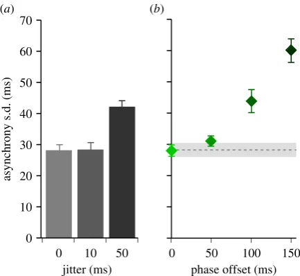
First, we manipulated metronome jitter to verify that asynchrony variability was affected, presenting a single metro-nome jittered by 0, 10 or 50 ms. We measured the asynchrony variability (s.d.) of the finger taps relative to the underlying unjittered metronome beats. As expected, increasing the jitter
resulted in higher asynchrony variability (F2,16¼37.6, p,
0.001; figure 3a).
Next, we considered synchronization performance when two metronomes (A and B) were simultaneously presented, one with high levels of jitter (50 ms) and the other only slightly jittered (10 ms). In particular, we focused on the zero phase-offset conditions and compared the asynchrony s.d. (averaged
over the two jitter conditions:f10, 50 msgandf50, 10 msg) to
that observed in the unjittered single metronome condition.
rspb.r
oy
alsocietypublishing.org
Pr
oc.
R.
Soc.
B
281
:
20140751
Using a paired t-test, we found no significant difference
between these two conditions (t8¼20.71,p¼0.497). Hence,
in contrast to the single metronome conditions where jitter sub-stantially impacted on participants’ performance, asynchrony variability remained low in the dual metronome condition, even though one of the metronomes was highly jittered. We further found no main effect of jitter on asynchrony s.d. (F1.2,9.5¼1.5, p¼0.255) when we analysed all condi-tions for the dual metronome presentacondi-tions. This means that asynchrony variability did not increase regardless of whether one of the metronomes was highly jittered or both were isochronous. These results highlight that participants were able to take advantage of the more reliable metronome to maintain their synchronization performance in the dual metronome conditions.
We found that, as predicted, an increasing phase offset between the two metronomes increased the asynchrony s.d. (F1.6,12.8¼27.1, p,0.001; figure 3b). While there was no
difference between 0 and 50 ms phase offsets (p¼0.311),
asynchrony s.d. increased significantly at phase offsets of
100 ms (p¼0.042) and 150 ms (p¼0.001). We suggest that
these results indicate two different strategies in participants’ synchronization. At low phase offsets, participants are inte-grating the two cues into a single beat estimate, with the outcome that the asynchrony s.d. remains low. However, as the phase offset increases, participants are treating the cues independently and switching between them. This switching incurs a substantial increase in asynchrony variability, regardless of the jitter applied to each metronome.
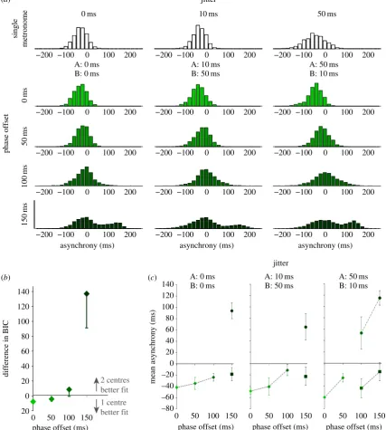
To examine these apparent strategies in more detail, we considered the distributions of asynchronies in each con-dition. Visual inspection indicated unimodal distributions at low phase offsets (suggesting integration of cues) and bimo-dal distributions at larger offsets (suggesting independent
targeting of the cues) (figure 4a). We quantified this
obser-vation by fitting two GMMs to each participant’s data: either with one centre (indicating a unimodal distribution) or two centres (indicating a bimodal distribution). The
difference between the BIC values for the two GMM models was calculated to establish which provided a better fit. We found that at low phase offsets (0, 50 ms), a unimodal distribution was more likely, while bimodal distribu-tions were more likely at 100 and 150 ms phase offsets
(figure 4b). Hence, it appeared that when the metronome
cues were separated by an offset of around 100 ms or greater, participants did not treat them as a common beat, but rather as independent beats. The bimodal distributions were a result of participants switching their finger taps to be in synchrony with either of the two sources.
We further calculated the mean asynchronies to under-stand how the timing of participants’ movements relative to the onsets of the metronome was affected by the experimental manipulations. We observed changes in mean asynchrony that depended on whether cues best fit a single or dual centred GMM, highlighting the different tapping strategies implemented by participants. For the low phase offsets, mean asynchrony was more positive for the 50 ms phase
offset than the 0 ms offset (F1,8¼9.31,p¼0.016; figure 4c),
indicating that participants were influenced by both metro-nome streams and hence integrating the cues. In situations where participants were more likely to show bimodal asynchrony distributions, we observed that one distribu-tion was centred around a negative asynchrony, the other was positive, close to the onset of the second metronome, highlighting the tendency to follow one cue or the other.
(b) Model fits to the experimental data
The experimental data suggest that human participants apply different strategies under the different experimental con-ditions: at low phase offsets, data is unimodal with low variance regardless of jitter condition, suggesting integration of the signals takes place. At high phase offsets, data are bimo-dal and suggest switching behaviour in the use of the two metronomes. This indicates that neither a scenario based on exclusively integrating the timing signals nor one based exclu-sively on selecting one signal over the other is sufficient to explain the participants’ behaviour. Formally, we tested two causal inference models and compared them against models of MI and MS. The first causal inference model (CI) inferred whether the auditory cues originated from a single beat or independent beats using the deviations between the signals caused by both a constant phase-offset and jitter
manipula-tions; the second (CIPA) assumed participants adapted to the
consistent phase offset between the cues and hence only based their inference on deviations due to the jitter. Using a global search optimization algorithm [25], we fit the four free parameters (see the electronic supplementary material, A, table S2) by minimizing the BIC of each participant’s data for each condition and model. Summing the BIC across con-ditions and averaging for each participant, we were able to compare how well each model explained the data.
We found that, overall, both causal inference models (CI
and CIPA) outperformed the MI and MS models (figure 5a)
in terms of the BIC. Specifically, we found that the causal inference models outperformed MI in all conditions and MS in all but one condition (phase offset: 0 ms, jitter:
f0, 0 msg; see table 1). The general goodness of fit measure
indicated the simulated data fit well with the experimental
data (figure 5b) and confirmed differences between the
0 10 20 30 40 50 60 70
asynchrony s.d. (ms)
jitter (ms) 0 10 50
phase offset (ms) 0 50 100 150
[image:6.595.54.271.41.240.2](a) (b)
Figure 3.
(
a
) Asynchrony s.d. to single metronome presentations. The
metro-nome was jittered by 0, 10 or 50 ms. Error bars show s.e.m. (
b
) Asynchrony
s.d. in the dual metronome conditions as a function of phase offset and
aver-aged across jitter conditions. Error bars show s.e.m. The horizontal grey bar
indicates the asynchrony s.d. in the isochronous single metronome condition,
+
1 s.e.m. (Online version in colour.)
rspb.r
oy
alsocietypublishing.org
Pr
oc.
R.
Soc.
B
281
:
20140751
models (F3,24¼2.736,p,0.001), with a significantly higher
r2of the CI
PAmodel over the MS and MI models (figure 5c).
Importantly, we found that the CIPAmodel outperformed
the CI model in terms of the BIC. This was surprising as the model describes the observer adapting to a fixed phase offset over the course of a trial and discounting this offset when determining whether or not the cues should be inte-grated. This appears contrary to our empirical results where overall participants’ strategies depended on the level of phase offset between the cues. This apparent contradiction can be accounted for by individual differences between
participants. In particular, the phase-offset threshold between integration of cues and treating them independently varied across participants, with a minority demonstrating better single-centre (i.e. integration) GMM fits to their distributions
even in the 150 ms phase-offset conditions. While the CIPA
model introduced an additional fixed parameter in the form of subtracting the phase offset from any estimated deviation between cues (see the electronic supplementary material, A), we noted that this was subsequently modulated by the free
parameter psingle (representing the prior probability of a
common single beat). Whilepsingleremained relatively constant
100
−200 −100 0 100 200 −200 −100 0 100 200 −200 −100 0 100 200
−200 −100 0 100 200 −200 −100 0 100 200 −200 −100 0 100 200
−200 −100 0 100 200 −200 −100 0 100 200 −200 −100 0 100 200
−200 −100 0 100 200 −200 −100 0 100 200 −200 −100 0 100 200
−200 −100 0 100 200 −200 −100 0 100 200 −200 −100 0 100 200
A: 0 ms B: 0 ms
A: 10 ms B: 50 ms
A: 50 ms B: 10 ms jitter
0 ms 10 ms 50 ms
phase offset
0m
s
single
metronome
50
ms
100
ms
150
ms
difference in BIC
100 150 50
0
2 centres better fit
1 centre
better fit 0 50 150
phase offset (ms) phase offset (ms) phase offset (ms)
phase offset (ms)
100 50 150
0 0 50 100 150
mean asynchrony (ms)
A: 0 ms B: 0 ms
A: 10 ms B: 50 ms
A: 50 ms B: 10 ms jitter
asynchrony (ms) asynchrony (ms) asynchrony (ms)
–80 –60 –40 –20 0 20 40 60 80 100 120 140
20 0 20 40 60 80 100 120 140 (a)
[image:7.595.84.512.48.524.2](b) (c)
Figure 4.
(
a
) Histograms of asynchronies from the experimental data. Negative asynchronies indicate the tap preceded the onset of metronome A. Histograms are
shown for each phase-offset condition (rows). Each column plots histograms for the different jitter conditions:
f
0, 0 ms
g
,
f
10, 50 ms
g
and
f
50, 10 ms
g
.
(
b
) Difference in Bayesian BIC values for GMM fits as function of phase offset. GMMs were fitted to each participant’s data with either one or two centres.
The goodness of fit of the data to each of the GMMs was measured using the BIC. The difference in BIC was calculated across conditions for each participant
and averaged to determine whether the histogram of data was more likely to originate from one or two distributions. Negative values indicate a better fit to
the single centred GMM; positive values indicate a better fit to the two centred GMMs. Error bars show s.e.m. (
c
) Mean asynchronies based on GMM centres.
Mean asynchronies were calculated based on the GMM centres that fitted best to each participant’s data. The figure shows the mean asynchronies for unimodal
distributions (diamond symbols) except where more than half the participants demonstrated better fits to bimodal distributions. Where this occurs, we plot the
mean of both centres (lower value, squares; higher value, circles). Plots are shown for each jitter condition. Error bars show s.e.m. (Online version in colour.)
rspb.r
oy
alsocietypublishing.org
Pr
oc.
R.
Soc.
B
281
:
20140751
across offsets for the CI model, it dropped as a function of offset
for the CIPAmodel (figure 5d). The effect of a reducedpsingle
value was to reduce the likelihood of judging a given pair
of signals to be a common single beat. Hence, the CIPA
model was more able to adapt to the different individual phase-offset thresholds for integration we observed across par-ticipants, than the CI model. This resulted in a better fit of the model to each participant’s data.
4. Discussion
Many simple and skilled actions depend on moving in time with signals that are embedded in complex auditory streams.
phase offset
0m
s
50
ms
100
ms
150
ms
asynchrony (ms)
asynchrony (ms) asynchrony (ms)
1 10 100 1000 10 000 100 000
CI MS
BIC difference (wrt CI
PA
)
0.4 0.5 0.6 0.7 0.8 0.9 1.0
goodness of fit (
r
2)
–200 0 200
–200 0 200
–200 0 200
–200 0 200
–200 0 200
–200 0 200
–200 0 200
–200 0 200
–200 0 200
–200 0 200
–200 0 200
–200 0 200
MI
CI
CIPA MS MI
p= 0.031 p< 0.001
0 0.1 0.2 0.3 0.4 0.5 0.6 0.7 0.8 0.9 1.0
0 50 100 150
prior Pr of common beat (
psingle
)
phase offset (ms)
(a) (b)
(c) (d)
A: 0 ms B: 0 ms
A: 10 ms B: 50 ms
A: 50 ms B: 10 ms jitter
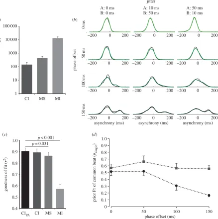
Figure 5.
(
a
) Difference in BIC scores for model fits, relative to the causal inference model with phase-offset adaptation (CI
PA). BIC scores were summed across conditions
for each participant. The three alternative models compared were: causal inference without phase adaptation (CI), mandatory separation (MS) of the cues and mandatory
integration (MI) of the cues. The difference between BIC scores for each model was calculated and averaged across participants. A positive value indicates that the model is
a worse fit to the data compared with CI
PA. (
b
) Simulated (CI
PAmodel) versus empirical PDFs. The empirical asynchronies (black dashed line) and simulated asynchronies
(shaded solid line) were pooled across all participants and converted to PDFs using a Gaussian kernel density estimation (KDE) algorithm. PDFs are shown for each
phase-offset condition (rows) and jitter condition (columns). (
c
) Goodness of fit of each model to the experimental data. Goodness of fit was calculated using an index between 0
and 1 by comparing BIC of the data to the model (
L
(
u
)) relative to: (i) a probability distribution of the data itself (
L
(Max)), and (ii) a random distribution
L
(Rand). Error
bars show s.e.m. (
d
) Mean value of the prior probability of a single common beat (
p
single) for each offset condition, averaged across participants and jitter conditions. The
[image:8.595.80.519.45.486.2]plot highlights the difference in
p
singlevalues for the CI (squares) versus CI
PA(circles) models. Error bars show s.e.m. (Online version in colour.)
Table 1.
Mean difference in BIC between the CI
PAmodel and the
mandatory separation (MS) model for each condition. (Positive values
indicate the CI
PAmodel is a better fit to the data.)
offset (ms)
jitter (A, B; ms)
0,0
10,50
50,10
0
2
18.2
3.5
8.3
50
21.4
13.4
18.5
100
48.1
40.7
45.2
150
130.9
104.7
23.0
rspb.r
oy
alsocietypublishing.org
Pr
oc.
R.
Soc.
B
281
:
20140751
Often these streams share an underlying rhythm but differ in temporal regularity and phase. Here, we tested how human movement synchronization to two simultaneously presented auditory metronomes was affected by differences in the phase and regularity between the two timing signals. We found that when the phase offset was low, participants showed evidence of integrating the signals, minimizing the variability in the timing of their responses. By contrast, when phase offset was high, responses were more variable and there was alternation in the response cue used for
synchronization (viz., bimodal distributions of movement
asynchronies; figure 4). This behaviour was well captured by a Bayesian causal inference model. The model used four free parameters and was able to explain situations in which participants chose to integrate signals or keep them separate. We applied two causal inference models to the data, one
con-sidering phase-offset adaptation (CIPA) and one without
adaptation (CI). Simulations indicated the causal inference models provided a better account for the experimental data than other models based on integration (MI) or selection (MS) only. The causal inference model incorporating phase-offset adaptation showed a better fit than the causal inference model without phase-offset adaptation. However, the free parameter describing the prior probability of considering the cues to form a single beat was found to be a function of
phase offset in the CIPAmodel. This suggests that the improved
fit resulted from this model being more flexible to differences in the phase-offset thresholds at which individual participants switched from integrating cues to treating them independently. Overall, the results suggest that humans exploit a Bayesian inference process to control movement timing in situations where the underlying beat structure of auditory signals needs to be resolved.
Evidence for optimal cue integration for multisensory sig-nals has been demonstrated across a range of tasks in both spatial and temporal contexts [11–13]. Moreover, multisen-sory cue integration has been shown to result in improved motor performance in a movement timing task [17,29,30]. This improvement was consistent with a maximum-likeli-hood model of integration based on the reliability of each sensory modality. However, an important step in this process involves deciding whether or not different sensory cues relate to the same environmental event: if not, the signals should be kept separate and not integrated [7–10]. Here, we focused on this process of deciding whether different sensory events relate to a common underlying beat. Our empirical data pro-vided evidence that participants do integrate two auditory signals into a single estimate of a metronome beat, but the probability of integration was a function of both the time offset between the signals and their relative temporal regula-rity. For instance, when participants tapped to simultaneous beats defined by two metronomes, with one jittered by 10 ms, the other 50 ms, the variability in finger-tap asynchronies remained equal to that when tapping to a single isochronous metronome. This demonstrated that synchronization varia-bility was reduced (relative to the individual signals) by integrating information from the individual (noisy) timing cues. This would not be expected if participants had simply switched between timing cues. Moreover, if participants had simply chosen the more reliable signal, the phase offset between the metronomes would not have been important. By contrast, we found an effect of phase offset, with move-ment asynchronies for the high phase-offset conditions (100
and 150 ms) producing bimodal distributions of movement timing, indicating that the two streams were treated indepen-dently at these high phase offsets. This highlights that a strategy based on integration alone could not account for the participants’ behaviour. We suppose two modes of behaviour—integration versus separation, with a causal infer-ence process that decided whether to integrate signals or treat them independently based on their relative reliability and temporal separation. The evidence for causal inference taking place was further corroborated by the single anoma-lous condition where we found causal inference did not provide the best fit. Namely, when the phase offset was zero and both metronomes were isochronous, we found that a causal inference model did not show a better fit than MS (table 1). This can be explained by the fact that the partici-pants only heard a single metronome cue in this condition (the tones overlap on every beat forming a dyad) and there-fore integration could not have taken place. The model was unable to account for this scenario and by integrating the cues described a lower expected variability than was observed, resulting in a poor fit. The predicted poor fit owing to this anomaly provides further evidence that causal inference is taking place in other conditions, where the fit is consistently better than the alternative models.
Exposure to a repeated, consistent asynchrony between multisensory cues has been demonstrated to result in tempo-ral recalibration, such that the point of subjective simultaneity is shifted to compensate for the offset [31]. We considered whether participants would, in a similar way, learn the con-sistent phase offset between the beats and recalibrate in terms of judging whether those cues defined a common beat or not.
We therefore tested two causal inference models: CIPAwhere
the phase offset is accounted for (i.e. not considered) when inferring the causality of the signals, and CI that included the phase offset in determining signal causality. We found
that the CIPAmodel showed a better fit than the CI model.
This was surprising given the empirical data showing an effect of phase offset on the distributions. Further examination
of the free parameters indicated thatpsinglebecame a function of
phase offset for the CIPAmodel (figure 5d). We suggest that
these results indicate that participants do not disregard the full phase offset in their inference of a single common beat,
but instead account for a proportion of the offset. The CIPA
model was more able to account for the differences across par-ticipants in the proportion of the phase offset accounted for and hence resulted in a better fit. The results from the model can be considered to show that participants generally underestimate the actual phase offset presented. Under similar circumstances, where repeated exposure to a temporal offset between multi-sensory cues results in temporal recalibration, it has also been found that an underestimation occurs in the recalibration, explained by a bias in a neural population coding model [32]. Finally, it is interesting to speculate about the cortical circuits underlying the behaviour we observed. There is evi-dence that different areas of the brain are recruited during beat processing versus duration or interval processing [2,33]: measuring absolute time duration recruits the inferior olive and cerebellum, while if intervals are regular (forming a beat) a striato-thalamo-cortical network is recruited [33]. Here, we added jitter to the metronomes such that the cues pre-sented varied from an isochronous beat (0 ms jitter) through to a highly unpredictable beat (50 ms jitter). Therefore, we may expect a switch from beat-based processing to duration-based
rspb.r
oy
alsocietypublishing.org
Pr
oc.
R.
Soc.
B
281
:
20140751
activations depending on the level of jitter applied to the metro-nome. However, by integrating the two cues into a single stream, temporal irregularity is minimized, which is likely to emphasize a beat-based structure. Minimizing the variability and extracting a beat maintains a predictive timing process (rather than reactive) [34], which is what we observed through the typically negative asynchronies to the cue onsets.
In conclusion, when synchronizing actions to auditory streams, people determine whether the cues define a common underlying beat or independent beats through Bayesian inference. As an extension of this work, it would be interesting to investigate the presence of causal inference
in real group settings (e.g. a string quartet [5]), using the foundations of the modelling work we have described here.
Experimental protocols were approved by the Science, Technology, Engineering and Mathematics Ethical Review Committee at the University of Birmingham.
Acknowledgements.We thank Konrad Ko¨rding for helpful suggestions on the development of our model, Ulrik Beierholm for comments on the draft manuscript and Dagmar Fraser for assistance in data collection.
Funding statement.This work was supported by Engineering and Phys-ical Sciences Research Council (EP/I031030/1) and Wellcome Trust (095183/Z/10/Z) grants.
References
1. Grahn JA, Rowe JB. 2012 Finding and feeling the musical beat: striatal dissociations between detection and prediction of regularity.Cereb. Cortex 23, 913 – 921. (doi:10.1093/cercor/bhs083) 2. Zatorre RJ, Chen JL, Penhune VB. 2007 When the
brain plays music: auditory-motor interactions in music perception and production.Nat. Rev. Neurosci. 8, 547 – 558. (doi:10.1038/nrn2152)
3. Grahn JA, Brett M. 2007 Rhythm and beat perception in motor areas of the brain.J. Cogn. Neurosci.19, 893 – 906. (doi:10.1162/jocn.2007.19. 5.893)
4. Mesgarani N, Chang EF. 2012 Selective cortical representation of attended speaker in multi-talker speech perception.Nature485, 233 – 236. (doi:10. 1038/nature11020)
5. Wing AM, Endo S, Bradbury A, Vorberg D. 2014 Optimal feedback correction in string quartet synchronization.J. R. Soc. Interface11, 20131125. (doi:10.1098/rsif.2013.1125)
6. Moore BCJ, Gockel HE. 2012 Properties of auditory stream formation.Phil. Trans. R. Soc. B367, 919 – 931. (doi:10.1098/rstb.2011.0355) 7. Ko¨rding KP, Beierholm U, Ma WJ, Quartz S,
Tenenbaum JB, Shams L. 2007 Causal inference in multisensory perception.PLoS ONE2, e943. (doi:10. 1371/journal.pone.0000943)
8. Shams L, Beierholm UR. 2010 Causal inference in perception.Trends Cogn. Sci.14, 425 – 432. (doi:10. 1016/j.tics.2010.07.001)
9. Sato Y, Toyoizumi T, Aihara K. 2007 Bayesian inference explains perception of unity and ventriloquism aftereffect: identification of common sources of audiovisual stimuli.Neural Comp.19, 3335 – 3355. (doi:10.1162/neco.2007.19. 12.3335)
10. Roach NW, Heron J, McGraw PV. 2006 Resolving multisensory conflict: a strategy for balancing the costs and benefits of audio-visual integration.Proc. R. Soc. B273, 2159 – 2168. (doi:10.1098/rspb. 2006.3578)
11. Ernst MO, Banks MS. 2002 Humans integrate visual and haptic information in a statistically optimal fashion.Nature415, 429 – 433. (doi:10.1038/ 415429a)
12. Alais D, Burr D. 2004 The ventriloquist effect results from near-optimal bimodal integration.Curr. Biol. 14, 257 – 262. (doi:10.1016/j.cub.2004.01.029) 13. van Beers RJ, Sittig AC, van der Gon Denier JJ. 1999
Integration of proprioceptive and visual position-information: an experimentally supported model.
J. Neurophysiol.81, 1355 – 1364.
14. Ban H, Preston TJ, Meeson A, Welchman AE. 2012 The integration of motion and disparity cues to depth in dorsal visual cortex.Nat. Neurosci.15, 636 – 643. (doi:10.1038/nn.3046)
15. Hillis JM, Ernst MO, Banks MS, Landy MS. 2002 Combining sensory information: mandatory fusion within, but not between, senses.Science298, 1627 – 1630. (doi:10.1126/science.1075396) 16. Knill DC, Saunders JA. 2003 Do humans optimally
integrate stereo and texture information for judgments of surface slant?Vis. Res.43, 2539 – 2558. (doi:10.1016/S0042-6989(03)00458-9) 17. Elliott MT, Wing AM, Welchman AE. 2010
Multisensory cues improve sensorimotor synchronisation.Eur. J. Neurosci.31, 1828 – 1835. (doi:10.1111/j.1460-9568.2010.07205.x)
18. Elliott MT, Welchman AE, Wing AM. 2009 MATTAP: a MATLABtoolbox for the control and analysis of
movement synchronisation experiments.J. Neurosci. Methods177, 250 – 257. (doi:10.1016/j.jneumeth. 2008.10.002)
19. Peters M. 1980 Why the preferred hand taps more quickly than the non-preferred hand: three experiments on handedness.Can. J. Psychol.34, 62 – 71. (doi:10.1037/h0081014)
20. Grotowski ZIB, Botev JF, Kroese DP. 2010 Kernel density estimation via diffusion.Ann. Stat.38, 2916 – 2957. (doi:10.1214/10-AOS799) 21. Matlab 2012 The Mathworks Inc., MA, USA. See
http://www.mathworks.com.
22. Vorberg D, Wing AM. 1996 Modeling variability and dependence in timing. InHandbook of perception and action(eds H Heuer, S Keele), pp. 181 – 262. London, UK: Academic Press.
23. Vorberg D, Schulze HH. 2002 Linear phase-correction in synchronization: predictions, parameter estimation, and simulations.J .Math. Psychol.46, 56 – 87. (doi:10.1006/jmps.2001.1375)
24. Repp BH. 2005 Sensorimotor synchronization: a review of the tapping literature.Psychon. Bull. Rev. 12, 969 – 992. (doi:10.3758/BF03206433) 25. Oldenhuis R. 2009 GODLIKE: a robust single-&
multi-objective optimizer. See http://www. mathworks.co.uk/matlabcentral/fileexchange/24838-godlike-a-robust-single-multi-objective-optimizer (accessed on 19 April 2013).
26. Schwarz G. 1978 Estimating the dimension of a model.Ann. Stat.6, 461 – 464. (doi:10.1214/aos/ 1176344136)
27. Stocker AA, Simoncelli EP. 2006 Noise characteristics and prior expectations in human visual speed perception.Nat. Neurosci.9, 578 – 585. (doi:10. 1038/nn1669)
28. Repp BH, Su Y-H. 2013 Sensorimotor
synchronization: a review of recent research (2006 – 2012).Psychon. Bull. Rev.20, 403 – 452. (doi:10. 3758/s13423-012-0371-2)
29. Wing AM, Doumas M, Welchman AE. 2010 Combining multisensory temporal information for movement synchronisation.Exp. Brain Res.200, 277 – 282. (doi:10.1007/s00221-009-2134-5) 30. Elliott MT, Wing AM, Welchman AE. 2011 The effect
of ageing on multisensory integration for the control of movement timing.Exp. Brain Res.213, 291 – 298. (doi:10.1007/s00221-011-2740-x) 31. Hanson J, Heron J, Whitaker D. 2008 Recalibration
of perceived time across sensory modalities.Exp. Brain Res.185, 347 – 352. (doi:10.1007/s00221-008-1282-3)
32. Roach NW, Heron J, Whitaker D, McGraw PV. 2011 Asynchrony adaptation reveals neural population code for audio-visual timing.Proc. R. Soc. B278, 1314 – 1322. (doi:10.1098/rspb.2010. 1737)
33. Teki S, Grube M, Kumar S, Griffiths TD. 2011 Distinct neural substrates of duration-based and beat-based auditory timing.J. Neurosci.31, 3805 – 3812. (doi:10.1523/JNEUROSCI.5561-10.2011) 34. Coull JT, Davranche K, Nazarian B, Vidal F. 2013
Functional anatomy of timing differs for production versus prediction of time intervals.Neuropsychologia 51, 309 – 319. (doi:10.1016/j.neuropsychologia. 2012.08.017)