Munich Personal RePEc Archive
Son Preference and Human Capital
Wang, Qingfeng
Nottingham University Business School China
8 January 2018
Online at
https://mpra.ub.uni-muenchen.de/95411/
Son Preference and Human
Capital
Qingfeng Wang
University of Nottingham Business School
ABSTRACT
We have developed a theoretical link between the existence of a son preference and the quantity
and quality of children. In our model, decisions about the quantity and quality of children are
interdependent and are influenced by a son preference. A son preference substantially widens the
gap between the quality of female and male children, and increases the possibility of having more
children to realize this preference. An increase in the level of son preference lowers the average
level of education, especially for female children. For households with a son preference, having a
female birth at each birth order significantly increased the probability of having more children,
with a magnitude which is much larger than that suggested in Dahl and Moretti (2008). More
interestingly, once such households have a son, there is a significant reduction in that household’s
likelihood of having more children. Furthermore, our findings establish the causal effect of a son
preference on the quantity and quality of children within a family as a son preference is found to
greatly reduce households’ sensitivity to the change in the shadow price of quantity as well as
quality.
Keywords: Son Preference; the Quantity and the Quality of Children
I.
Introduction
“Awoman’s virtue is to have no talent”女子无才便是德1。
There is a large amount of literature on growth models which highlights the importance of gender
inequality (as a result of gender preference) in economic growth2 through the channel of human
capital differentiation between different genders. The impacts of gender differences have been
observed in many different domains, perhaps most notably in labor market (e.g., Blau and Kahn
2000). Gender inequality (or gender preference) is deeply rooted in countries with a large fraction
of its population depends on agriculture for its livelihood, in patrilineal societies and cultures with
a tradition of ancestor worship, and it has also found a foothold in some developed economies3.
One form of gender inequality is perfectly mirrored in the son preference cultures around the world.
Son preference is more obvious and more severe in some countries than in others. For example,
the son preference culture is much stronger in Asian countries4 than in Western Europe. We have
focused specifically on the son preference because of its impact on the human capital, and hence
on economic growth, and because the previous research has little to say about the mechanism
underlying the impacts of a son preference on the quantity and quality of children. The quantity
and quality of children are often inspired by specific demand. Empirical evidence indicates that
children from larger families have lower average educational attainments. However, such evidence
does not explain why children within a family may have very different levels of education
regardless of family size. It is intriguing, although challenging, to understand why some families
choose to have more children but others do not, and more importantly, how the underlying
1The original quotation reads: “眉公曰:丈夫有德便是才,女子无才便是德。此语殊为未确。” (出自清·张岱
《公祭祁夫人文》).
2For example, Lagerlöf 1999; Galor and Weil 1996; Barro 1991; Bloom and Williamson 1998; Taylor 1998; Barro and Lee 1994; Barro and Sala-i-Martin 1995; Dollar and Gatti 1999; Forbes 2000; Lorgelly and Owen 1999; Knowles et al. 2002.
3According to a 2011 Gallup survey and a Pew report, a son preference also occurs in the U.S. And, a continuous son preference was observed in Finland among the national majority and the Swedish speaking minority (Andersson et al. 2007).
rationales that bolster decisions to have more children have a cause effect on both the family size
and the quality of children.
In his seminal paper on the theory of fertility choice, Gary S. Becker (1960) introduced fertility
choice into the realm of economic analysis. Since then, children have been treated as consumer
durables. Although Becker acknowledged that preferences may vary across households, the impact
of a preference such as gender preference on endowment and on any interactions between the
quantity and quality of children was not addressed in his papers, nor in any papers with coauthors.
The literature that extends the quantity and quality model introduced by Becker (1960) is quite
extensive; despite this, however, they fail to capture the effects of the essential parental
characteristics on the quantity and quality of children. We believe that it is crucial to include these
parental characteristics in the quantity-quality model as they could affect both family size and children’s educational outcome5.
The family environment is widely believed to be a primary factor in determining children’s educational outcomes (Black et al. 2005). In some societies, the son bears the responsibility of
continuing the family line, which is a critically important aspect of the “quality” of a child that
parents are looking for in these cultures, and males are in general have higher earning power than
females, which can also lead to a preference for sons over daughters (Qian 2008). We believe that
a son preference is a very important component of a family environment, and it has some causal
effects on the quantity and quality of children within a family. But, how does the son preference
affect households’ decisions on both the quantity and quality of children? We argue that to answer
this question, it is essential to account for the fact that parents in societies with a strong son
preference culture value sons more than daughters6.
5Family size and children’s educational outcome can be endogenously determined by parents. In societies with no compulsory education system, children’s education attainment is decided by their parents according to, for example, differentiated labor market returns to education for men vs. women and family’s need in labor supply from their children.
We develop a theoretical link between the existence of a son preference and the quantity and
quality of children. In our model, the quantity and quality decisions about children are
interdependent and are influenced by a son preference. A son preference substantially widens the
gap between the quality of female and male children in households with a son preference, and
increases the possibility of having more children to realize this preference. An increase in the level
of son preference lowers the average level of education, especially for female children. In this article, we conduct several empirical tests showing the importance of this channel in households’ decision in the quality and quantity of children.
Our analysis has yielded the following findings. Foremost, irrespective of how our findings are interpreted, we have shown that children’s gender matters in terms of households’ decisions about their educational outcomes and about the number of children to have. After controlling for a
number of factors, ranging from geographic locations7 to variables which measure regional
economic developments, we found that female children receive significantly lower levels of
education than their male siblings. We have taken the following approach to distinguish the causal
effect of a son preference on the quality of children. We have compared the quality of children of
opposite sexes by using multiple birth samples (where members of twins or triplets from each
household were of opposite sexes), while also controlling for family background characteristics.
By doing so, we addressed the following two concerns. First, the issue of endogeneity, which is
the educational investment in each child is decided by parents, and hence may be related to other
unobservable parental and other family characteristics. By using multiple birth data, we were able
to control for these characteristics as these twins (triplets) would have concurrently experienced
similar changes in the unobservable parental and other family characteristics. Second, using the
multiple birth data helped to alleviate concerns that any differences in the quality of male and
female children was as a consequence of significant changes in the socioeconomic and educational
environment for children of different genders and of a different age or because children from the
same family would have both inherited very different intellectual ability from their parents8. Doing
so yielded an even wider gap in the quality of female and male children.
Second, we find that for households with a son preference, having a female birth at each birth order
significantly increased the probability of having more children, which is much larger than that
suggested in Dahl and Moretti (2008). More interestingly, once such households have a son, this
reduces significantly the probability of having more children, and this negative effect ranges from
5.6% to 41.8% depending on the birth-order of the son.
Third, the strong existence of a son preference in rural China compared to that found in urban areas
can be explained by the paramount differences between the two areas in terms of such factors as the distinctive features of China’s welfare system9 and the fact that job opportunities are more concentrated and diverse in urban areas. Such differences between the two areas have shaped the
large differences in people’s perceptions of the quality of children of different genders. Based on
these clear differences, we were able to quantify the level of son preference in rural China, where
the estimated son preference in rural China ranged between 0.20 and 1 across the three waves of CHIPS, where earlier years’ rural samples are associated with a stronger son preference.
A final observation is in order. As we have used Chinese data to estimate empirically the impact
of a son preference on the quality and quantity of children, we need to highlight the differences
between the son preference culture in China and other countries. Although, son preference culture
is not unique to China, as shown by Dahl and Moretti (2008) who concluded that parents in the
U.S. favor boys over girls, we argue that the nature of China’s son preference differs significantly
from other countries. Son preference may originate from cultural considerations, as well as factors
such as a concern for care of the elderly, but in China, many people continue to endorse the
8Both the boys and the girls from pairs of twins (triplets, quadruplets and so on) were free from their parents’ gender preference, so they receive unbiased and equal care during pregnancy; and more importantly, twins (triplets, quadruplets and so on) share either some or all of the same genomes, so we have strong reason to believe that they will have inherited very similar intellectual ability from their parents.
traditional belief that “there are three unfilial things in your life, and to leave no posterity10 is the worst” (Shi 1982). China has a strong son preference culture in its rural areas (Goodkind 2015), where many villagers’ lifetime goal is to have sons (Li 1995; Wasserstrom 1984). The strength of
the son preference in China is partially evidenced in Amartya Sen’s book ‘More than 100 Million
Women Are Missing’. Furthermore, other factors (e.g. economic factors) fail to explain the highly
skewed sex ratio at birth (SRB) observed in Asian countries, as none of the developed economies,
with the exception of South Korea11, has a SRB above 1.10. A number of studies has confirmed
that the highly skewed SRB in China is largely due to the persistent and strong son preference
culture in China (Ebenstein 2010; Chen et al. 2013; Wang 2019). If this is how the son preference
works in China, it suggests a very different mechanism from that which seemingly functions in
other countries, such as in the U.S.
Our findings are related to three bodies of literature. First, by estimating empirically the level of
son preference, our study contributes to the small but growing body of literature on the persistence
of this phenomenon (Shi 2009; Ebenstein and Leung 2010;Almond et al. 2013; Hu and Tian 2018;
Zhang 2019). Second, our study is related to previous research examining the impact of a son
preference on educational attainment and parents’ investment in their children (e.g., Rosenzweig
and Schultz 1982; Chen et al. 1981; Das Gupta 1987; Ahmad and Morduch 1993; Thomas 1994;
Burgess and Zhuang 2001; Park and Rukumnuaykit 2004; Kugler and Kumar 2017; Barcellos et
al. 2014). Our findings show that a son preference both lowers significantly the average level of
education, and has a very large negative impact on the quality of female children.
Third, our study augments the literature regarding the tradeoff between the quantity and quality of
children, as pioneered by Gary S. Becker. What sets our study apart from that of Becker and his coauthors’ works, as well as others (e.g. Qian 2009; Black et al. 2005), is that we have incorporated the son preference into the relationship between the quantity and quality of children, and we have
found that a son preference exerts significantly more impact than that of the quantity of children
10Having no posterity refers to having no son, as ancestor worship is an important part of Chinese culture (Schwartz 1985), and it needs to be performed by male descendants. Having no male descendants means the discontinuation of the line of ancestry.
on children’s quality. Our findings also suggest that, in societies with a son preference, the quantity
and quality of children interacts largely because parents in the process of realizing their son
preference need to adjust their decisions about the quantity and quality of their children. A son
preference can play a critical role in the interaction between the quality and quantity of children
because: 1) it greatly reduces households’ sensitivity to the change in the shadow price of quantity
as well as quality, and 2) the expected sizable increase in households’ marginal utility owing to
the realization of a son preference.
The implications from both our theoretical model and empirical findings confirm that the son
preference is the driving force behind the gender gap in education in China. Based on our analysis,
we have found that a son preference affects the quality of children more than the quantity of
children, and it also affects both the shadow price of quality and the shadow price of quantity12.
The rationale behind this is that in a strong son preference culture, a son is considered to carry the
intrinsic quality (or ability) of providing more economic returns to the family than would be the
case for a daughter, to continue the family line and to provide care for elderly family members
and/or fulfill any inheritance requirements. Therefore, parents with a son preference are more
likely to stop producing children only when they have at least one son13. When more births are
required to realize the son preference, an increase in the quantity of children inevitably lowers the
quality of children, especially the quality of daughters. Within their particular budget constraints,
having a son is the priority of the household with a strong son preference, while such households
are less demanding about the quality of their children compared to those with no clear gender
preference, all else being equal. The negative relationship between quantity and quality is robustly
confirmed to be negatively correlated across households, however, households with a son
preference are found to differentiate strategically on the quality of their children based on their
gender rather than to want approximately equal levels of quality for each of their children.
12Recall that: an interaction between the quantity and quality that causes significant changes in both shadow price of quantity and of quality is the key element that generates a trade-off between quantity and quality.
Therefore, the proposition endorsed by Becker 1960; Becker and Lewis 1973; Willis 1973; Becker
and Tomes 1976; Rosenzweig and Wolpin 1980, that “the quantity and quality of children interact because parents tend to want approximately equal levels of quality for each of their children” is, in general, not supported among households with a son preference.
Our paper proceeds as follows: the next section describes the data, and Section III outlines the
identification strategies in estimating the results. Section IV reports the estimations and discusses
the findings, and section V develops the model, and presents the implications suggested by the
model. Finally, Section VI presents the conclusion.
II.
Construction of the datasets
2.1The data sample
In estimating the impact of a son preference on the quality and the quantity of children, we made
use of three out of the seven waves (1988 to 2013) of the Chinese Household Income Project
Survey (CHIPS), namely those from 1988, 1995 and 2002. These are seven years apart, which we
consider to be a time period which is neither too short nor too long for the purposes of comparison
studies between the different waves. Those individuals surveyed in the first two waves were largely
free from the impact of the one-child policy and the ‘Nine Years Compulsory Education System’14,
while the one-child policy had more of an impact on the 2002 wave than the other two, the impact
was still much milder compared to those in later years. This justifies the use of only the first three
waves of survey data. Each survey collected data from households selected randomly from both
rural and urban populations, and they covered very large and extensive geographic areas in China.
The information of all members of each household is recorded. Each survey contains household
information on their income, expenditure, and demographics, as well as geographic information,
occupational information, assets and so forth. A more detailed description of each of the seven
waves of the survey is reported on the official website of the China Institute for Income
Distribution at Beijing Normal University.
The units of observation are children, to which we link the demographic information of their
parents and the household level information from each CHIPS, accordingly. We constructed 18
subsamples in total from the three waves of CHIPS, which were divided equally between both the
rural population and the urban population, as well as between the three waves of CHIPS. The size
of each sample depends on both the original size of the surveys and the number of missing values
of the key variables of interest, and the associated control variables. Some summary statistics of
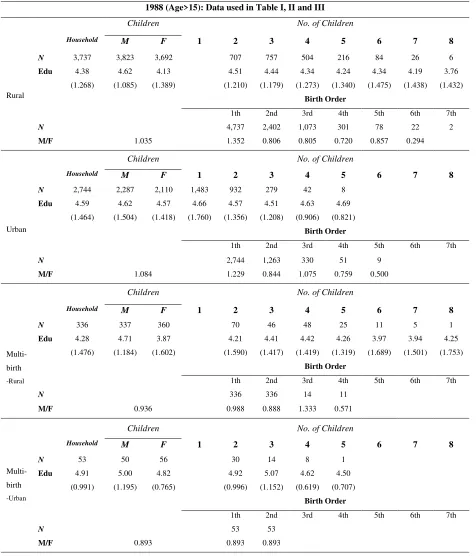
the samples are presented in Table A1 in the Appendix.
2.2 Data to estimate the effect of a son preference on the quality of children
To investigate the impact of a son preference on the quality of children, we constructed data on
some of the children included in each of the three waves15. As children from rural areas in China
are raised and educated in socioeconomic, cultural and educational environments which are very
different from those in urban areas, we studied separately the impact of a son preference on the
quality of children for rural populations and urban populations.
The key variables of interest are children’s education attainment (i.e. their level of education), their
gender, and the number of children in a household. The dependent variable is the level of
educational attainment. We have used the level of educational attainment as a measure of the
quality of a child in relation to a son preference because the number of years a child is in education
prior to the introduction of the ‘Nine Years Compulsory Education System’ in China is largely
determined by the parents’ willingness to invest in their children’s education, and such decisions
may be based on gender. The more years in education, the greater the loss of the anticipated income
from the labor supply of the children, which discourages parents from providing more education
and, more importantly, from providing equal educational opportunities for all children. The earlier
their children can begin working, the sooner they can contribute to the family, and this is a
convincing strategy to follow when the returns from education are not considered by rural
populations to be favorable, and parents are not obliged to send their children to school. However,
it should be noted that the educational inequality between genders narrowed considerably alongside China’s rapid economic development. In addition, the ‘Nine Years Compulsory Education System’, which took effect in late 1986, helped both to significantly enlarge the student
population, and to reduce the drop-out rate of students, especially that of female students, even in
the rural areas (Ding 2012).
The education level16 (education attainment) is coded from 8 to 1, where 8 represents the highest
level of education (university level). For the gender variable, males are coded as 0, while females
are 1. In our study, to control for demographic as well as regional effects on the quality of children,
we also included the fathers’ education attainment17, a variable called minority18, the family
income, and variables featuring geographic characteristics and locational information.
We extracted a total of 12 subsamples from the three waves of CHIPS, to enable the study of the
effect of a son preference on the quality of children. More specifically, for each wave, we compiled
two samples for the rural population and two for the urban population. For both the rural and the
urban samples, the larger sample contained all children with no missing values on the variables
mentioned above, while the smaller sample contained only data on twins, triplets, quadruplets and
so on, of opposite sexes19. However, we did not distinguish between the different types of twins20,
triplets, quadruplets and so on. The multiple births sample was used to confirm the robustness of
the results from using the larger sample.
2.3Data to estimate the effect of a son preference on the quantity of children
16In more detail, the education level was coded as 1 for someone who had never attended formal education, 2 for the lower elementary school (below year 3), 3 for upper elementary school, 4 for junior middle school, 5 for senior middle school (including professional middle school), 6 for technical secondary school, 7 for junior college, and 8 for college/university.
17Using mothers’ education level did not lead to qualitatively different results. 18
There are 56 ethnic groups in China, with the Han group considered as the majority. All other ethnic groups are considered as a minority.
19For example, we stipulated that they are twins of opposite sexes.
To investigate the impact of a son preference on the quantity of children, we first used the six
larger samples constructed in Section 2.2 respectively for both the rural and urban populations.
Here, the number of children in a household taken as the dependent variable (i.e. the quantity of
children). We also included the fathers’ level of educational attainment, the minority variable, the
family income, and the other control variables in the regression analysis. The key variables of
interest are gender and quality (i.e. the educational attainment of a child).
The CHIPS data sets we use provide information on each child of a household and contain a panel
component. To take advantage of this, we construct six additional samples which incorporated a
dummy typed variable, called SonDummy21. The SonDummy variable helps to distinguish
households with a son preference from those possess no clear son preference in their decisions on
whether or not to have another child after the birth of a son. The SonDummy variable, together
with the gender of each child sorted by their birth order, were used to capture the impact of the son
preference on the quantity of children by considering both the impact of the birth of a son and the
sex composition of the current children on the quantity of children. We included in the samples as
many children’s observations as possible, by including only the following variables in the
robustness test, namely the quantity of children, the gender of the children, and the SonDummy22.
We could do this because both the independent variable gender and the SonDummy have very
small correlations with the other independent variables, and the inclusion or exclusion of the other
independent variables did not qualitatively change the results. By doing so, we dropped very few
children’s observations from each wave of CHIPS. In estimating the effect of a son preference on
the quantity of children, children of all ages are included in the study.
III.
Identification
21To construct the SonDummy variable, we first sorted the children of each household according to their birth order, and numbered the first-born child as 1, the second-born child as 2, and so on.The SonDummy takes the value of zero, corresponding to the female children who were born to a household before the first-born male, while it takes value of 1 once a son has been born into the family. The number of observations of the SonDummy equals the number of children in a household.
22
The following reduced form analyses were employed to empirically estimate the impact of the son
preference on both the quality and quantity of children.
3.1Using gender to identify the effect of a son preference on the quality of children
We consider the impact of the gender of a child on the quality of children is a natural candidate to
use to represent the son preference of a household. The son preference of a household will be
reflected in the differentiated quality of children, measured by their educational attainment, with their parents as the ‘investors’ in their children’s education. All else being equal, a household with a son preference is likely to invest more in the education of their sons than in their daughters. The
presence of such an effect is confirmed if gender exerts a significantly negative impact on the
quality of those female children.
China is a vast country with huge discrepancies in the development of socioeconomic and
education system across its provinces, and even across counties within a certain province.
Therefore, we have included geographic dimensions in capturing factors other than a son
preference in the study of the quality of children. The trade-off between the quality and the quantity
of children suggests the inclusion of the quantity of children in the study. We therefore propose
the following reduced form equation, which will be used to estimate the impact of a son preference
on the quality of children:
Quliaty𝑖𝑗𝑘𝑤= 𝛼1𝑘+ 𝛼2𝐺𝑒𝑛𝑑𝑒𝑟𝑖𝑗𝑘𝑤+ 𝑎3𝑄𝑢𝑎𝑛𝑡𝑖𝑡𝑦𝑗𝑘𝑤+ 𝛼4𝐸𝑑𝑢𝐹𝑎𝑡ℎ𝑒𝑟𝑗𝑘𝑤+ 𝛼5𝑀𝑖𝑛𝑜𝑟𝑖𝑡𝑦𝑗𝑘𝑤
+ 𝛼6𝐼𝑛𝑐𝑜𝑚𝑒𝑗𝑘𝑤+ 𝛼7(𝐿𝑜𝑐𝑎𝑡𝑖𝑜𝑉𝑎𝑟𝑖𝑎𝑏𝑙𝑒𝑠𝑗𝑘𝑤) + 𝐴𝑔𝑒𝐷𝑢𝑚𝑚𝑦𝑖𝑗𝑘𝑤+ 𝜖𝑗𝑘𝑤.
(1)
We regress the quality of children (i.e. quality of child 𝑖 of household 𝑗 who lives in area 𝑘 - either
rural or urban, and who is taken from the survey data collected in year 𝑤) on gender, the quantity
of children and other controls. The variables with four digits of subscript are individual level data,
and variables with three digits of subscript are household level data. The father’s educational
attainment is used to control for a household’s level of endowment. The ethnic minority groups
enjoy preferential treatment from the Chinese government, such as exemption from the population
meaningful to distinguish households from ethnic minorities. Minority is a dummy variable, which
is equal to zero if a household is Han, and equal to one where it belongs to another ethnic group.
Unlike most other countries, China’s hukou system clearly defines each individual’s resident status
as either rural or urban, which distinguishes individuals, for example, in their eligibility for access
to public health and other welfare systems. Therefore, there was no difficulty in identifying
whether an individual is from a rural or an urban area. Our locational variables comprise
information about the geographical features surrounding the areas where households are situated.
They also contain information on whether a rural resident is living closer to cities, which helps to
differentiate those rural households who live closer to cities than other rural households from the
same county but further away from cities. These locational variables and other household level variables allow us to difference out household specific characteristics that are affecting children’s education. All explanatory variables are confirmed to either have very small correlations or the
absolute value of the correlations was approximately 0.30. To control for cohort effects, we include
indicator variables for age groups in the regressions. We estimated equation (1) for both rural and
urban samples, and for those samples containing only twins (triplets and so on), and for samples
containing all types of households.
3.2Identifying the effect of a son preference on the quantity of children
To obtain a quantitative estimate of the effect of a son preference on the quantity of children, we
first estimated the following reduced form equation.
Quantity𝑗𝑘𝑤 = 𝛽1+ 𝛽2𝐺𝑒𝑛𝑑𝑒𝑟𝑖𝑗𝑘𝑤+ 𝛽3𝑄𝑢𝑎𝑙𝑖𝑡𝑦𝑖𝑗𝑘𝑤+ 𝛽4𝐸𝑑𝑢𝐹𝑎𝑡ℎ𝑒𝑟𝑗𝑘𝑤+ 𝛽5𝑀𝑖𝑛𝑜𝑟𝑖𝑡𝑦𝑗𝑘𝑤+
𝛽6𝐼𝑛𝑐𝑜𝑚𝑒𝑗𝑘𝑤+ 𝛼7(𝐿𝑜𝑐𝑎𝑡𝑖𝑜𝑛𝑉𝑎𝑟𝑖𝑎𝑏𝑙𝑒𝑠𝑗𝑘𝑤) + 𝜈𝑗𝑘𝑤. (2)
Quantity𝑗𝑘𝑤 is the number of children of household 𝑗 from area 𝑘 (either rural or urban) and is taken from CHIPS data in year 𝑤. The key independent variables of interest are gender and quality.
We regress the quantity of children on children’s gender, the quality of children, and other controls.
An increase in the quality of children exhausts some of the resources which may otherwise be used
in producing more children, therefore, quality is expected to have a negative effect on Quantity𝑗𝑘𝑤.
having a son by having more children before they have a son, and thus a positive gender effect on
Quantity𝑗𝑘𝑤 would capture this effect.
Using specially constructed samples, we conducted the following reduced form analysis using
Poisson regression, both to validate the earlier findings, and also to understand the households’
underlying rationales in determining the number of children.
Quantity𝑗𝑘𝑤 = 𝛾1+ 𝛾2𝐵𝑖𝑟𝑡ℎ𝑂𝑟𝑑𝑒𝑟𝐹𝑒𝑚𝑎𝑙𝑒𝑖𝑗𝑘𝑤+ 𝛾3𝑆𝑜𝑛𝐷𝑢𝑚𝑚𝑦𝑖𝑗𝑘𝑤+ 𝜂𝑗𝑘𝑤. (3)
The quantity of children is regressed on the 𝐵𝑖𝑟𝑡ℎ𝑂𝑟𝑑𝑒𝑟𝐹𝑒𝑚𝑎𝑙𝑒𝑖𝑗𝑘𝑤 and 𝑆𝑜𝑛𝐷𝑢𝑚𝑚𝑦𝑖𝑗𝑘𝑤. The
𝐵𝑖𝑟𝑡ℎ𝑂𝑟𝑑𝑒𝑟𝐹𝑒𝑚𝑎𝑙𝑒𝑖𝑗𝑘𝑤 is a dummy variable which represents the gender of the 𝑖𝑡ℎ born child in
household 𝑗 from area 𝑘 and is taken from CHIPS wave 𝑤.𝐵𝑖𝑟𝑡ℎ𝑂𝑟𝑑𝑒𝑟𝐹𝑒𝑚𝑎𝑙𝑒𝑖𝑗𝑘𝑤 is equal to
zero if the 𝑖𝑡ℎ born child is female, and is equal to one if it is male. To differentiate between cases
where a son joined different households at a different birth order, a dummy type variable
𝑆𝑜𝑛𝐷𝑢𝑚𝑚𝑦𝑖𝑗𝑘 was introduced into the regressions. The 𝑆𝑜𝑛𝐷𝑢𝑚𝑚𝑦𝑖𝑗𝑘 was assigned a value of
either zero or one to each child depending on whether a son has been born to a household. All
female children born before the first-born male were assigned a value of zero, and once a son had
been born to a household all subsequent births, including the first-born male, were assigned with
a value of one. The merit of this variable is that it signifies the impact of the first-born male on a household’s decision of how many children to have. A significant 𝑆𝑜𝑛𝐷𝑢𝑚𝑚𝑦𝑖𝑗𝑘 indicates strongly that the level of a son preference is important in determining the household’s decision
about the number of children to have. Using data selected by a birth order variable23 for each round
of estimations, we were able to uncover the impact of gender on the quantity of children at different
birth orders. The gender effect on the quantity of children is validated by 1) both the gender of the
child at each birth and the SonDummy or 2) independently by the two. Having no son motivates a
household to have an additional child in the hope that their son preference can be realized. Consequently, a child’s gender at each birth could have a noticeable influence on the total number of children produced by a household with a son preference.
IV.
Estimations
4.1The effect of a son preference on the quality of children
The children in the 1988 and 1995 samples only include those who were over 18 years old,
therefore, the results derived using these two samples are largely free from the impact of the
one-child policy and the ‘Nine Year Compulsory Education System’, and at the age of 18 it is very
likely that the individual has completed formal education given that the average education level in
China was quite low prior to 1978 (=1995-18). We report the estimation results in both Table 1
and 224.
The results concerning rural populations are reported in Table 1. In 1988, on average, girls from
rural areas received at least one and a half years 25 less education than boys, and about a half year
less in 1995. We interpret these findings as strong evidence that a child’s gender matters for their
level of education, given that the average schooling was only approximately 7.326 years in both
1988 and 1995. What is more striking is that before 200227, a child’s gender was, in general, found
to have played a more decisive role than the quantity of children in determining a child’s
educational attainment. Although the quantity of children has significant coefficients of between – 0.221 and – 0.037 for most subsamples, these numbers, on average, suggest a much smaller
24
The estimated results without using the indicators for age groups are presented in the Table A2 and A3 in the appendix. Those results are not qualitatively different from that has been reported in both Table 1 and 2 respectively. 25This is calculated as 0.496 ×3≈ 1.5, where 3 is the average number of years for each education level.
reduction in the average educational attainment of the children than is the case for gender in the earlier years’ samples.
Table 1
The effect of a Son Preference on the Quality of Children for Rural Populations a – with indicator
variables for age groups
1988 1995 2002
Larger Sample Multiple Births Larger Sample Multiple Births Larger Sample Multiple Births
Gender – 0.496*** (.0271)
– 0.808*** (.0988)
– 0.171*** (.0212)
– 0.218* (.1394)
– 0.062** (.0267)
– 0.203 (.1515) Quantity – 0.061***
(.0107)
– 0.099*** (.0372)
– 0.037*** (.0117)
– 0.221** (.0889)
– 0.117*** (.0155) 0.029 (.1350) Education (Father) 0.165*** (.0083) 0.117*** (.0320) 0.131*** (.0097) 0.015 (.0878) 0.219*** (.0122) 0.1282 (.1080) Minority – 0.239***
(.0514)
– 0.158 (.2039) 0.279*** (.0403) 0.996** (.4095) 0.205*** (.0369) 0.325 (.2689) Family income 0.00003*** (.000005) 0.00005*** (.00001) 0.00001*** (.000002) 0.00001 (.00001) 0.00002*** (.000001) 0.00002 (.00001) Terrain28 – 0.055***
(.0201)
– 0.318*** (.0795)
– 0.046*** (.0145)
– 0.059 (.1438)
Geographic location29
0.050 (.0579)
– 0.085 (.2294) Old
Revolutionary Areas
– 0.027 (.0423)
– 0.019 (.1325)
– 0.013 (.0259)
– 0.2478 (.2774)
Suburb 0.183
(.1087)
0.576* (.2962)
– 0.270*** (.0515)
– 0.502* (.2855)
Impoverished Areas
– 0.274*** (.0393)
– 0.158** (.0677)
– 0.110*** (.0213)
– 0.589*** (.2198)
Province – 0.008*** (0.0011)
– 0.004 (0.0044)
– 0.005*** (.0008)
0.009 (.0079)
0.000000001 (.000000009)
– 0.0000003 (.0000007)
N 7,515 697 7,221 119 6,963 105
a Data from the Chinese Household Income Project Surveys. Quality of children is the dependent variable. Multiple-birth
samples were abstracted from the original larger samples. Standard errors in parentheses. ***, **, * indicates statistical significance at 1%, 5% and 10%, respectively.
28Terrain includes the land features: 1. Plain; 2. Plateau; and 3. Mountainous region. Data was not available for the 1995 and 2002 samples.
As the one-child policy abruptly intervened in the process of human reproduction by imposing a
limit on the number of children a household could have, the insignificant gender effect identified
in the 2002 sample is not necessarily an indication that a significant change had taken place in the
son preference culture in rural China, but rather is an indication of the effect of the one-child policy in limiting the number of children, while the ‘Nine Year Compulsory Education System’ left rural households with little room to exercise their son preference by differentiating their children’s level
of educational attainment based on their gender.
As a robustness check, we used multiple-birth samples which only contained twins, triplets and so
on (e.g. members of each set of twins, triplets, etc., were required to be opposite sexes) to test for
the son preference effect on the quality of children. Gender is confirmed to be the single most
important factor used by parents in rural China in determining each of their children’s level of
educational attainment. We believe that the high dropout rates of girls had nothing to do with the
level of difficulty of subjects at school, given that most of the children in the 1988 and 1995
samples only completed their education at a level below senior middle school. We conclude that
the additional number of years’ education provided to male children from rural families was an
intentional act by parents at the cost of their female children. The human capital loss of the female
children is not an accidental coincidence given that twins, triplets and so on of opposite sexes are,
on average, not very different from each other in their inheritable genomes, and hence their ability
to complete a basic level of education30. The significant loss in human capital, as a result of
receiving an inadequate level of education, is very likely to be an adverse consequence of the son
preference. The results are remarkably robust and are in line with what we expected.
It is important to note that all independent variables in Table 1 have reasonably small correlations
with each other, and more importantly, the gender variable has small absolute correlations of
approximately 0.10 with any of the other independent variables. The results concerning the effect
made by gender on the quality of children remain unchanged and significant if we drop any or all
of the independent variables, which further confirms the robustness of the explanatory power of
the gender variable on the quality of children.
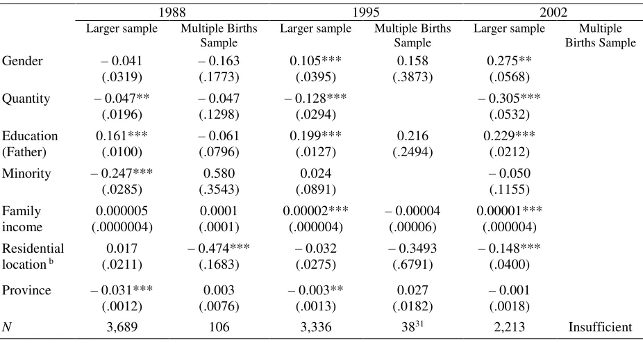
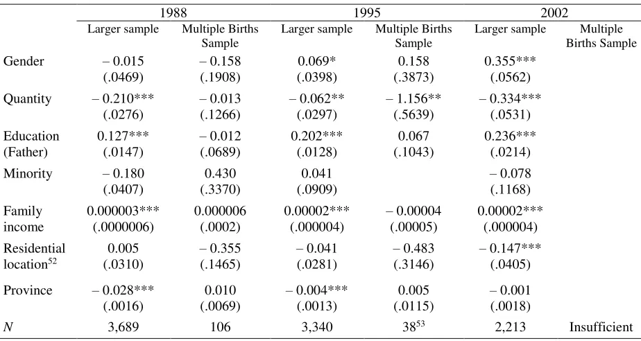
Table 2
The effect of a Son Preference on the Quality of Children for Urban Populations a– with indicator
variables for age groups
1988 1995 2002
Larger sample Multiple Births Sample
Larger sample Multiple Births Sample
Larger sample Multiple
Births Sample
Gender – 0.041 (.0319)
– 0.163 (.1773) 0.105*** (.0395) 0.158 (.3873) 0.275** (.0568) Quantity – 0.047**
(.0196)
– 0.047 (.1298)
– 0.128*** (.0294)
– 0.305*** (.0532)
Education (Father)
0.161*** (.0100)
– 0.061 (.0796) 0.199*** (.0127) 0.216 (.2494) 0.229*** (.0212) Minority – 0.247***
(.0285)
0.580 (.3543)
0.024 (.0891)
– 0.050 (.1155) Family income 0.000005 (.0000004) 0.0001 (.0001) 0.00002*** (.000004)
– 0.00004 (.00006)
0.00001*** (.000004) Residential
location b
0.017 (.0211)
– 0.474*** (.1683)
– 0.032 (.0275)
– 0.3493 (.6791)
– 0.148*** (.0400)
Province – 0.031*** (.0012)
0.003 (.0076)
– 0.003** (.0013)
0.027 (.0182)
– 0.001 (.0018)
N 3,689 106 3,336 3831 2,213 Insufficient
aData from the Chinese Household Income Project Surveys.
b Residential location is specified as: 1. City center; 2. City; 3. Suburbia; 4. Exurbia.
Quality of children is the dependent variable. Multiple-birth samples were abstracted from the original larger samples. Standard errors in parentheses. ***, **, * indicates statistical significance at 1%, 5% and 10%, respectively.
For the rural sample, the quantity of children was found to exert significantly negative effects on
the quality of children, but the magnitude of its effect on the quality of children was overshadowed
by the gender effect. Children from households with fathers who had a higher level of educational
attainment on average received relatively higher levels of education. The government’s
preferential treatment of minority ethnic groups took effect on the quality of children in the later
waves of CHIPS. Meanwhile, children who lived in mountainous areas, impoverished areas and
less economically developed provinces32 attained lower levels of education compared with other
children living in better economically developed areas of China.
31For the multiple-birth sample, we intentionally dropped the minority variable to ensure a sufficient number of observations could be used for the regression analysis.
The results concerning urban populations are presented in Table 2. Contrary to the findings from
the rural samples, a son preference was not confirmed to have a significant impact on the quality
of children in our urban samples. More specifically, no significant difference between the
educational attainment of male children and female children was evident from the 1988 CHIPS
data, while female children even obtained slightly higher levels of educational attainment than
male children in the 1995 CHIPS data, and in 2002 they had significantly surpassed male children
in their level of educational attainment. We believe that this change from females being at a
significant disadvantage in their education in rural areas, to females enjoying more equality in
urban areas is a result of the shift from a very strong son preference environment to an environment
which is more gender equal and/or gender tolerant. These contrasting results between the rural and
urban areas sheds some light on the merit of our use of gender to capture the effect of a son
preference on the quality of children. The educational attainment of a person who lives in an urban area is more likely to be determined by the child’s keenness to study and perform at school, as well as their family’s attitude towards education and the household resources. By the comparison of the educational attainment of children of both genders and from rural and urban areas, a
significant negative gender effect on the quality of children provides strong evidence of the
presence of a son preference in rural China.
4.2The effect of a son preference on the quantity of children
The total number of children in a household is likely to be determined by its economic wellbeing,
the expected quality of the children, as well as its associated demographic, social and cultural
factors, and other random factors. The total number of children to have is unlikely to be decided
at the outset of a marriage, and the ideal and realized family size may differ significantly from
each other. The process, from the first-born to the last-born, will take many years to complete in a
changing environment. Our findings are able to shed some light on the potential mechanisms
underlying these choices.
Although gender is found to have a positive effect for both the rural and urban samples, this does
not necessarily imply that a son preference existed in both areas. This is because, for instance, a
cultures, which is not specified in the reduced form model (2) used to estimate the results in Table
3. We argue that the results in Table 3 may be informative about the sign of the relationship
between child’s gender and the quantity of children, but not about its magnitude, as the elasticity
[image:21.612.75.542.200.660.2]also depends on the birth order of the first-born son.
Table 3
The effect of a Son Preference on the Quantity of Children
1988 1995 2002
Rural Urban Rural Urban Rural Urban
Gender 0.220***
(.0310) 0.018 (.0238) 0.175*** (.0211) 0.093*** (.0231) 0.176*** (.0201) 0.085*** (.0223)
Quality – 0.061*** (.0128)
– 0.074*** (.0097)
– 0.040*** (0.0119)
– 0.021** (.0101)
– 0.066*** (.0092)
– 0.045*** (.0079) Education (Father) 0.034*** (.0095) 0.096*** (.0087)
– 0.041*** (.0098)
0.008
(0.0077)
– 0.018* (.0096)
0.003
(.0086)
Minority 0.359***
(.0584)
0.072***
(.0242)
– 0.174*** (.0410)
0.040
(.0529)
– 0.206*** (.0286)
0.133***
(.0462)
Family income 0.0001***
(.000006)
0.000001***
(.0000003)
0.00002***
(.000002)
– 0.00003 (.00003)
0.00001***
(0.000001)
0.000008
(.000001)
Terrain 0.011
(.0227) 0.039*** (.0147) Old Revolutionary Areas
– 0.118*** (.0476)
0.012
(.0264)
Suburb – 0.092
(.1224)
– 0.085*** (.0524)
Impoverished
Areas
0.198***
(.0447)
– 0.104*** (.0217)
Residential
location
0.040**
(.0184)
– 0.013 (.0164)
0.042***
(.0160)
PROVINCE – 0.013*** (0.0012)
– 0.014*** (.0010) 0.005*** (0.0008) 0.002** (.0007) 0.0000008*** (.00000007) 0.002*** (.0007)
a Data from the Chinese Household Income Project Surveys. Standard errors in parentheses. Quantity of children is the
dependent variable. ***, **, * indicates statistical significance at 1%, 5% and 10%, respectively.
Given that the results regarding the gender effect on the quantity of children remain qualitatively
unchanged, with or without the other independent variables, this enabled us to only make use of a
more parsimonious model (3) compared to that used in Table 3 for the estimation of the gender
effect on the quantity of children.
A nonlinear Poisson regression33 and sorting the sample by birth orders were employed to account
for the fact that the dependent variable is a count measure and a probabilistic feature of the decision
making faced by each household when deciding on the number of children to have. The results are
presented in Table 4. It is important to note that because we have used children of all ages in
estimating the results in Table 4, the one child policy itself could have a negative impact on the
quantity of children. Therefore, some cautions need to be taken in interpreting the findings.
Each column reports the estimation results specifically based on the observations corresponding
to each birth order. The progressive nature of the decision making for the number of children is
well captured by both independent variables. For the independent variables, Row1 reports their
coefficients, Row 2 reports the clustered robust standard error, and Row 3 reports the marginal
effects in a semi-elasticity form. For indicator variables, such as our two independent variables,
the marginal effect represents the percentage change in the probability of having more children
when the indicator variable moves from zero to one. Overall, the previous results concerning
gender on the quantity of children remained qualitatively unchanged. With regard to the urban
population, the gender effect for each birth order on the quantity of children is found to be
insignificant across the three waves of urban samples (see columns (4), (5) and (6) in Table 4).
For rural households where the first-born is a girl, the estimates in column (1) suggest that their
probability of having two or more children is significantly higher than that of the first-born son
families across the three wave of CHIPS, with these probabilities ranging from 16.9% to 30%. It
is interesting to note that the probability is higher in the later years’ samples across the three
surveys. Three observations are in place: first, the higher probability of rural households having
two or more children in the later years’ samples, if the first child is a girl, clearly indicates that the
level of son preference is not decreasing in China’s rural areas; second, a sharp rise in income
within a short space of time does not necessarily lead to a sizable reduction in the level of son
preference in societies with a traditionally strong son preference; third, the one-child policy has
aggravated the urgency of those households with a son preference to have two or more children to
realize having a son, even if that meant breaching the one-child policy, if their first child was a
girl. This also explains why the one-child policy was not effective in reducing China’s fertility rate
during its earlier years (e.g. Zhang 2017; Wang 2019).
The estimates in column (2) imply that, for households in which the first two children are girls,
the probability of having three or more children is higher than for those families which already
had a son. The probability ranges from 0.3% to15.2% across the three waves of CHIPS, where the earlier years’ rural samples are associated with a larger probability. The later years’ rural samples having a smaller or even statistically insignificant probability of having three or more children is
intuitive, because the one-child policy was implemented more strictly in its later years and the
authorities kept a close eye on those who had already breached the policy. Severe punishments,
ranging from stiff financial fines, the confiscation of property, and even forced abortions
(Jimmerson 1990) were imposed on many such “lawbreakers”. As a consequence, we suspect that
the statistically insignificant probabilities of having three or more children in the later years’
sample is a result of the one-child policy. By comparison, using the U.S. census data, Dahl and
Moretti (2008) reported a statistically insignificant probability of having two or more children, if
the first child was a girl, and reported a probability of having three or more children at only 0.6%
higher than the first-born son families34. The estimates in column (3) suggest that, in households
with no son, the probability of having four or more children was higher than for those families in
which at least one of their first three children was a boy, with the probability ranging from 9.1%
to13.4% across the three waves of CHIPS, although this was only significant statistically in 198835.
Table 4
The effect of a Son Preference on the Quantity of Children – Poisson regression
1988
Rural Urban
(1) (2) (3) (4) (5) (6)
Birth order (of girl) 1 0.063*** (.0124) 0.169 0.010 (.0181) 0.016 2 0.051*** (.0147) 0.152 0.020 (.0263) 0.046
3 0.034*
(.0212)
0.124
0.044
(.0442)
0.142
SonDummy – 0.081***
(.0178) –0.243
– 0.061*** (.0212) –0.227
– 0.056* (.0309)
0.130
0.039
(.0513)
0.126
Log likelihood – 13547.88 – 13537.64 – 8183.21 –10201.91 – 4973.82 – 1460
VIF36 1.77 1.96 1.00 1.86 1.50
N 9,653 8,212 4,857 7,644 3,469 936
1995 Birth order (of girl) 1 0.143*** (.0124) 0.295 0.011 (.0262) 0.012 2 0.018 (.0209) 0.045 -0.002 (.0713) -0.004
the level of son preference in China is much stronger than in the U.S., and the social environment in China is more tolerant towards gender inequality than in the U.S.
35We suspect that the statistically insignificant probability of having four or more children in 1995 and 2002 was a result of the one-child policy.
3 0.028
(.0299)
0.091
Son Dummy – 0.169***
(.0251) –0.418
– 0.048 (.0356)
-0.160
– 0.015 (.0891) –0.032
Log likelihood – 10991.94 – 7827.63 – 3070.23 – 5662.77 – 710.84
VIF 1.38 1.43 1.39
N 7,515 5,301 1,942 5,294 5,37 Insufficient
2002
Birth order
(of girl)
1
0.160***
(.0163)
0.300
0.009
(.0240)
0.012
2
0.001
(.0215)
0.003
0.0004
(.0467) 0.0008
3 0.04
(.0325)
0.134
0.011
(.1431)
0.033
SonDummy -0.134***
(.0265) – 0.324
0.017
(.0429) 0.056
– 0.028 (.0552)
0.059
– 0.015 (.1635) –0.047
Log likelihood – 11767.75 – 7333.53 – 2469.91 – 6465.59 – 1632.09 – 171.75
VIF 1.35 1.36 1.38 1.76
N 8,312 5,010 1,556 5,635 1,211 113
a Data from the Chinese Household Income Project Surveys. Standard errors in parentheses. Quantity of children is the
dependent variable. Top panel: Poisson regression for 1988 for each birth order and for both rural and urban samples
separately. Middle panel: Poisson regression for 1995 for each birth order and for both rural and urban samples separately.
Lowest panel: Poisson regression for 1995 for each birth order and for both rural and urban samples separately. ***, **, *
indicates statistical significance at 1%, 5% and 10%, respectively.
The estimates in column (2) concerning the SonDummy variable suggest that having a son in the second birth significantly reduces rural households’ probability of having three or more children ranges from 24.3% to 41.8%, compare to households with their first two children are girls. The
households with their first three children are girls, although it is only statistically significant in
1988 rural sample.
V.
Model
The reduced form analysis establishes the responsiveness of important decisions in the quantity
and quality of children to changes in sex composition of their children and the birth of the first son.
However, empirical findings have little information about the mechanism underlying the decisions
of households. The model we have developed allows us to uncover the underlying mechanism of
how a son preference affects both the quantity and the quality of children, and how a son preference
changes the interactions between the two. To capture analytically the effects of a son preference
on the quantity and quality of children, a model is required which is embedded within this
heterogeneity of fertility and differentiated quality of children across households with or without
a son preference. Therefore, it seems useful to go beyond Becker and his coauthors’ models to
account for the issues arising out of differences in household choices due specifically to their
different levels of son preference.
Similar to Becker and Tomes (1976), we assume that a household has a utility function with the
following form:
𝑈 = 𝑈(𝑛, 𝑄, 𝑦) (4)
where 𝑛 is the number of children, Q represents quality of each child in the household, and 𝑦 the
aggregate amount of all other commodities. A household faces the following budgetary constraints:
𝐼 = 𝑝𝑦𝑦 + 𝑝𝑞𝑛𝑞
,
(5)where 𝑝𝑦 is the price of 𝑦, 𝑝𝑞 the average cost of increasing 𝑞 by one unit, and 𝐼 is the total family
income. Therefore, 𝑝𝑦𝑦 is the total expenditure on the aggregate amount of all other commodities,
and 𝑝𝑞𝑛𝑞 is the total cost of children.
𝑛 = ⌊𝑛̅(𝜉)⌋⏟ (𝑎)
or ⌈𝑛̅(𝜉)⌉⏟
(𝑏)
.
Here, 𝑛̅(𝜉)is the average number of children born into households which possess no son preference
and share a similar characteristic ξ, such as geographic location, income and parents’ education
level, where the floor and ceiling function is defined respectively as ⌊𝑥⌋ = max{𝑚 ∈ 𝕫| 𝑚 ≤ 𝑥}
and ⌈𝑥⌉ = min{𝑚 ∈ 𝕫| 𝑚 ≥ 𝑥}.
For households with a son preference, we have assumed their decision about the number of
children to have is jointly determined by the sex composition of their children after each birth37
and other controlling factors (e.g. budget constraints, educational resources). In the following, we
have assumed that once a son has been born into households with a son preference, they will
behave very similarly in their fertility rate to those households with no gender preference. We
propose that such households’ decisions about the number of children to have is governed by the
following equation, based on the rationale that more births are expected for households with a son
preference where no son has already been born,
𝑛 = ⌊𝑛̅(𝜉) × (1 + 1⏟ 𝑆𝑜𝑛(𝑛̅(𝜉)) × 𝑆)⌋
(𝑎)
or ⌈⏟ 𝑛̅(𝜉) × (1 + 1𝑆𝑜𝑛(𝑛̅(𝜉)) × 𝑆)⌉
(𝑏)
(6)
where 1𝑆𝑜𝑛(𝑛̅(𝜉)) is an indicator function which equals one if none of the children in 𝑛̅(𝜉) is a
boy, and otherwise it equals zero. Therefore, the term 𝑛̅(𝜉) × 1𝑆𝑜𝑛(𝑛̅(𝜉)) × 𝑆 measures the
number of additional children38 that households with a son preference intend to have to realize
their son preference compared to those households with no son preference and possess similar
characteristic 𝜉. Here, 𝑆 signifies the level of a son preference, which is defined as:
37For example, the decision whether to have an additional child for households with a son preference depends on whether a son has been born into the households.
38The additional number of children is in the range of [0,⌈𝑆 × 𝑛̅(𝜉)⌉],where the upper bound of the interval depends
on the households’ level of son preference. It is equal to zero when there is already a son born into the family.
Assuming that no son has been born into households with a son preference, on average, the additional numbers of
children will be translated into a probability of having at least one son, which is the range of [0.75, 1 − (1
2)
⌈𝑆×𝑛̅(𝜉)⌉
𝑆 ∈ (0, 𝜂); if a household possesses a son preference (7)
𝑆 = 0; otherwise.
An individual’s level of 𝑆 is partially determined by the level of intrusiveness of their surrounding environment in personal matters and the social attitude towards genders. The appreciation of the
expected future value of a son is formed through learning and interactions with members of social
communities.
We modify Becker and Tomes’s (1976) assumption that the “the quality of each child is the same”
to assume that the quality of each child is either perceived very similarly or very differently by each household, depending on their level of son preference. The households’ utilities are, to some extent, determined by the level of their son preference. Following this line of reasoning, we
differentiate our definition of the quality of children from Becker and Tomes (1976) by
incorporating the effect of a son preference on the perceived quality of a child from the parents’
perspective. This is defined as:
𝑄𝑖 = 𝑒 +∑ 𝑞𝑗
𝑛 𝑗=1
𝑛 (1 + 1𝑆𝑜𝑛(𝑖) × 𝑆) = 𝑒 + 𝑞 + 𝑞 × 𝑆 × 1𝑆𝑜𝑛(𝑖)
(8)
where 𝑄𝑖 is (an element in the set 𝑄) the quality of the 𝑖𝑡ℎ child, 𝑞 (=∑ 𝑞𝑗
𝑛 𝑗=1
𝑛 ) captures the households’ intention to contribute equal levels of quality to each of their children, and 𝑒 (i.e. the innate ability – the endowment) is assumed to be fixed for a household and it is considered as
exogenous and independent of 𝑞. In addition, 1𝑆𝑜𝑛(𝑖) is an indicator function which equals one if
the 𝑖𝑡ℎ child is a boy, and otherwise it equals zero. Therefore, equation (5) reveals the parents’
differentiation in the quality of their children based on their gender, where a female child receives
approximately an average level of the households’ contribution (which is assumed to be equal to
𝑞) towards their quality, but a male child receives preferential treatment subject to the parents’ level of son preference. The term 𝑞 × 𝑆represents a household’s perceived additional “quality”39
of a son compared to a daughter.
For a given level of son preference40 and a fixed 𝑝𝑞, the household chooses the aggregate amount
of all other commodities, the number of children 𝑛, and the level of quality of children 𝑄, to
maximize the utility function in equation (4), subject to the budget constraints (5), son preference
conditions (7), and the quality function (8). The maximization yields41:
𝑀𝑈𝑦 = 𝜆𝑝𝑦 = 𝜆𝜋𝑦
𝑀𝑈𝑄𝑖 =
𝜆𝑛𝑝𝑞
1+𝑆×1𝑆𝑜𝑛(𝑖) =
𝜆𝜋𝑄
1+𝑆×1𝑆𝑜𝑛(𝑖)= 𝜆𝜋𝑄
′
𝑀𝑈𝑛 = 𝜆𝑞𝑝𝑞 = 𝜆𝜋𝑛
(9)
𝑀𝑈𝑆 = 𝑀𝑈𝑛× 𝑛̅(𝜉) × 1𝑆𝑜𝑛(𝑛̅(𝜉)) × 1𝐵(𝛽) + 𝑀𝑈𝑄𝑖× 𝑞 × 1𝑆𝑜𝑛(𝑖)
where 𝑀𝑈’s are the marginal utilities, 𝜆 is the marginal utility of income, 𝜋𝑄′ is the “adjusted”
shadow price of the quality of children dependent on the household’s level of son preference, and
𝜋𝑛 is the shadow price of the quantity of children. It is important to note that our 𝜋𝑄′ can be significantly smaller than the shadow price of the quality of children 𝜋𝑄 (= 𝑛𝑝𝑞) defined in Becker
and Tomes (1976), and the difference between 𝜋𝑄′ and 𝜋𝑄 depends on the household’s level of son
preference. The impact of preferences for male offspring to female offspring on sex ratio at birth
is obvious in son preference cultures, such as China and South Korea – as evidenced in their
heavily skewed sex ratio at birth in China (since 1990) during the one-child policy as well as in
South Korea from 1987-2006 (e.g. Wang 2019). This observation of a strong male preference at
birth reinforces the importance of the potential discrepancy between 𝜋𝑄′ and 𝜋𝑄 as a result of a son
preference.
Although both the shadow price of the quality of children, 𝜋𝑄′ and 𝜋𝑄, are directly related to the
quantity of children, 𝜋𝑄′ is deemed to be less sensitive to the quantity of children than the 𝜋𝑄
derived under the framework of Becker and Tomes (1976). An increase in the quantity of children
inevitably increases the expenditure on children, however, to accommodate the increase in the cost
of raising more children when more births appear to be a sine qua non for having a son, households
40The level of son preference can range from it being better to have sons than daughters, to it being essential to have at least one son.
with a strong son preference are keener than other households on redistributing their resources
among their children based on their gender. When it becomes economically unsustainable because
of the large number of (female) children born before a son, households with a strong son preference
may either embrace sex-selective abortions and/or the abandonment of baby girls (when the legal
and social environments are tolerant of abortions and the abandonment of baby girls), or
substantially reduce investment in their daughters to have one more child for the purposes of
having a son. The additional number of children a household plans to have is subject both to their
level of son preference and to any budget constraints, all else being equal.
The shadow price of the quantity of children, 𝜋𝑛, is related to the quality of children. The higher
the quality of children a household aims to achieve, the higher the cost of an additional child. For
households with a son preference, for the purposes of having a son, they may reduce their
contribution to the quality of their daughters to offset the increase in cost because of the need to
have more children before having a son. Consequently, each daughter in such a household is likely
to receive a discounted household contribution towards her quality, where the severity of the
discount will depend on the level of son preference of the household. We found that the son
preference reduces the social income42 of a son-preference household by𝑆𝑒𝜋𝑄
1+𝑆, which signifies the potential loss of the household’s genetic endowment due to the son preference. Furthermore, it is
important to note that the endowment loss of 𝑆𝑒𝜋𝑄
1+𝑆 is related to the household’s total number of children, its level of genetic endowment and the son preference. For a given level of endowment,
an increase in both (either) the number of children and (or) the level of son preference can cause
substantial loss in social income as raising the quality of more children becomes more expensive,
which further intensifies the unequal distribution of resources between sons and daughters.
Considering a society as a whole, its aggregate loss in social income from households with a son
preference can be enormous43. In addition, as a persistent and strong son preference culture
42Household’s social income is defined as 𝜋
𝑦𝑦 + 𝜋𝑛𝑛 + 𝜋𝑄′𝑄 = 𝐼 + 𝜋𝑄′𝑄. Hence, the difference between the two
social incomes with and without son preference equals to the difference between 𝜋𝑄′𝑄 = 𝜋𝑄(𝑒 + 𝑞) for 𝑆 =
0, and 𝜋𝑄′𝑄 = 𝜋𝑄
1+𝑆(𝑒 + 𝑞(1 + 𝑆)), that is 𝜋𝑄(𝑒 + 𝑞) − 𝜋𝑄
1+𝑆(𝑒 + 𝑞(1 + 𝑆)) = 𝑆𝑒𝜋𝑄
1+𝑆.